COVID-19: Data-Driven Mean-Field-Type Game Perspective


Learning & Game Theory Laboratory, Center on Stability, Instability and Turbulence, New York University Abu Dhabi, P.O. Box 129188 Abu Dhabi, UAE
Games 2020, 11(4), 51; https://doi.org/10.3390/g11040051
Submission received: 29 July 2020
/
Revised: 18 October 2020
/
Accepted: 26 October 2020
/
Published: 3 November 2020
(This article belongs to the Special Issue Mean-Field-Type Game Theory)
Abstract
:In this article, a class of mean-field-type games with discrete-continuous state spaces is considered. We establish Bellman systems which provide sufficiency conditions for mean-field-type equilibria in state-and-mean-field-type feedback form. We then derive unnormalized master adjoint systems (MASS). The methodology is shown to be flexible enough to capture multi-class interaction in epidemic propagation in which multiple authorities are risk-aware atomic decision-makers and individuals are risk-aware non-atomic decision-makers. Based on MASS, we present a data-driven modelling and analytics for mitigating Coronavirus Disease 2019 (COVID-19). The model integrates untested cases, age-structure, decision-making, gender, pre-existing health conditions, location, testing capacity, hospital capacity, and a mobility map of local areas, including in-cities, inter-cities, and internationally. It is shown that the data-driven model can capture most of the reported data on COVID-19 on confirmed cases, deaths, recovered, number of testing and number of active cases in 66+ countries. The model also reports non-Gaussian and non-exponential properties in 15+ countries.
1. Introduction
COronaVIrus Disease 2019 (COVID-19) is one of the severe acute respiratory syndrome-related coronavirus. COVID-19 is a disease caused by the virus SARS-CoV-2. SARS-CoV-2 is infecting people across several countries within a few months and causing deaths, economic losses and food insecurity. As COVID-19 spreads around the globe, authorities are making decisions about local migration, confinement, isolation, quarantine and healthcare system capabilities. Individuals, depending on the country, culture, social-economic context, age and season, are also making decisions concerning COVID-19. In this paper, we propose an integrated mathematical model and analysis strategies for combatting the propagation of COVID-19 and for examining the economic consequences. For each infected person, one often defines the number of secondary infections that are generated by that patient. The probability distribution of the latter random variables is referred to as offspring distribution. The offspring distribution depends on its infectiousness which can be biological, environmental, behavioral or combinations of these. The offspring distribution has been estimated from empirical data for outbreaks of several infectious diseases such as tuberculosis, cholera, plaque, smallpox, severe acute respiratory syndromes (SARS), MERS and Ebola. There are two important sectors that authorities are considering to mitigate COVID-19. The public health sector which tries to understand the dynamics of COVID-19 (via epidemiological models and efforts) and take measure to flatten the curve of hospitalized COVID-19 patients (mitigation and suppression). In this case, flattening the pandemic curve basically means reducing the number of people who are hospitalized all at once so that the local healthcare system is not overburden. The economic policy sector has been used to alleviate negative consequences implied by COVID-19 and by the restrictive policy measures. The economic policies are also being used to prevent the amplification and the multiplication of the crisis. Unfortunately, these two sectors and approaches have not been coordinated enough. The effectiveness of the public health measures may depend on the perception of people in practice and their expectations because each individual also make its own decisions. Therefore both decisions, from economic policies by authorities and from country-specific individual preferences, should be integrated all together.
1.1. Literature Review of SARS-CoV-2
There is an important ongoing research on COVID-19. Below we review some closely related works. For SARS-CoV-2 (and hence COVID-19) the offspring distribution is not known and the COVID-19 data set is dynamic. The public data set is updated on a regularly basis or so, meaning it changes over time as new information becomes available. Below we highlight some features considered in prior works.
- Effect of mobility on the propagation COVID-19: The movement and migration of people between locations add an additional difficulty in estimating the infectivity as each infected person may be moved, flown to another city, state, country or continent. Some estimations have been proposed by using contact-tracing or mobile tracking of the path of the each infected person and all its possible contacts using mobile networks and recognition. However, these estimations on COVID-19 remain limited at a global level [1,2,3,4]. The work [5] focuses on a Global Epidemic and Mobility model that integrates sociodemographic and population mobility data set in a spatially structured stochastic disease approach to simulate the spread of epidemics at the worldwide scale. In contrast to [5], we integrate a data-driven optimization setup for authorities and for individuals as well.
- Age and gender structure on COVID-19 death rate: Because the COVID-19 reported deaths depend on ages and gender, the role of demography on COVID-19 spread and fatality is examined in [6]. The work in [7] explains the use of SARS-CoV-2 RT-PCR testing outcomes in Italy. The work in [8] provides some early estimates of clinical severity of COVID-19 by age.
- Epidemiological data set is needed during epidemics to best monitor and anticipate spread of infection. The work in [9] provides geo-positioned records of case of of COVID-19 outbreak. COVID-19-related deaths are not clearly defined in the international reports available so far, and differences in definitions of what is or is not a COVID-19-related death might explain some of the variations in the reported data.
Several basic compartmental models have been suggested in the literature to simplify the complexity of mathematical modelling of infectious diseases. These include
- SIR (susceptible-infected-removed),
- SEIR, that is extended SIR with exposed (E) agents
- SEIR with quarantine (Q)
- SEIR with age-structure
- SEIR with spatial location
- SEIRD that is R is divided into recovered (R) or deceased (D)
- SEIRD with data fitting via parameters.
These models need to be adapted to include important and key features of COVID-19 such as context-awareness, decision-making, co-morbidities per area, mobility, age, gender, healthcare status, and testing capabilities to capture the evolving COVID-19 data set [3,10,11,12,13] and to improve the strategies by considering risk-awareness. Other related works on non-linear modelling can be found in [14,15,16,17].
We propose a data-driven model that integrates some of the basis of economic and pandemic issue. Table 1 displays some of the key differences and key features of the data-driven mean-field-type game (MFTG) model.
1.2. Mean-Field-Type Game Theory
The term ’mean-field’ refers to a physics concept that attempts to describe the effect of an infinite number of particles on the motion of a single particle. Researchers began to apply the concept to social sciences in the early 1960s to study how an infinite number of factors affect individual decisions. However, the key ingredient in a game-theoretic context is the influence of the distribution of states and or control actions into the payoffs of the decision-makers. There is no need to have a large population of decision-makers. A mean-field-type game (MFTG) is a game in which the (instantaneous) payoffs and/or the state dynamics coefficient functions involve not only the state and actions profiles but also the distribution of state-action process (or its marginal distributions).
In a mean-field-type game, the quantities-of-interest (such as instantaneous payoff, cost, performance functionals, state kernel/coefficients) depend not only on the type-state-actions of the decision-makers but also on the distribution of them. This allows us to consider higher order (non-linear) dependence in the distribution of state and or actions on the expected utility/cost functions. It also allows us to capture risk-awareness in the performance metric whenever one or more decision-makers are facing uncertainties. We refer the reader to [18,19,20,21,22,23,24,25,26,27,28] for more details on MFTG.
1.3. Data-Driven Mean-Field-Type Game Theory
Below, we build on the MFTG model a data-driven methodology. The data-driven mean-field-type game theory (MFTG) model of the pandemic COVID-19 presented here is built upon Markov decision process model of epidemics. Despite the simplicity of this model, important features are extracted that can assist potential decisions on the strategy to combat the outbreak, essentially configuring a scenario ranging from short-term suppression to long-term mitigation depending on the achieved reduction in the hospitalized number, contact number, exposed number, testing number, pre-existing health conditions, age, gender, location, mobility pattern and spatial contact rate. A coopetition and dedicated effort from individuals, governments, decision-makers and stakeholders will help in reducing the propagation but with a cost despite the increased rate of recovered people.
Basically, data-driven MFTG is given as follows.
- Time is continuous
- Data is reported at discrete-time instants.
- Decision-makers: individuals, firms and authorities
- Control Actions: Individuals’ actions include contact/meeting rates and a movement path to go outside for food, pharmacies or other basic needs. Firms’ action include the production essential, moderate-essential and less-essential goods and total working hours. An authority at specific location controls the testing actions and migration rates within that area, between different areas of a city or between cities or the country level.
- Objective: an individual aims to reduce its risk of being hospitalized and to limit its economic consequences. Each firm aims to maximize its revenue while keeping its employees from infections. Each authority aims to reduce the number of deaths under cost-benefit considerations (see Figure 1).
1.4. Contributions
The proposed data-driven MFTG model has the following key features
- context-awareness: captures some areas/city/country-specific and comorbidity features
- integrated decision-making and risk-aware cost-benefit analysis for authorities and individuals.
- the mobility map/pattern per areas/cities/countries is endogenous to the data-driven model
- the country-specific age-structure is endogenous to the data-driven model
- the pre-existing health conditions per city/country is endogenous to the data-driven model
- an estimation of the probability of being exposed (coughing, sneezing, talking, surface contact)
- the hospital capacity is endogenous to the model. It is an aggregated data from number of hospital beds, intensive care facilities, ventilators, nurses, doctors, point-of-care etc.
- the testing capacity per country is endogenous to the data-driven model (the number of testing per week, number of testing facilities per areas/city/country)
- the infection status of the untested individuals is endogenous to the data-driven model
The goal of the article is to examine the data-driven MFTG modelling aspect of COVID-19. From the mean-field-type game theory perspective, one examines carefully each individual process at the microscopic level. The individual characteristics are age, gender, location, and infection status. As each infected individual may affect its evolving neighbors and path, it creates an evolving mean-field term at the local, regional, national and international level. Thus, a macroscopic description of the proportion of infected per location will emerge as a global mean-field term. In addition, risk-awareness at the individual level as well as the global level is proposed. As several countries may not have the same seasons, culture or socio-economic context, we introduce temperature field, seasonal variation and local specificities across the countries and couple them with the decisions on the duration of the soft/medium/hard confinement. The age-structured dynamics are introduced to capture the dependence on age and on the prior medical conditions of the COVID-19 patient. For the pandemic COVID-19, many local hospitals cannot sustain a massive influx of infection and this will create a congestion and saturation. Saturation and the local capacities of the healthcare system are introduced into the model and de-congestion and curve flattening strategies are analyzed. We also examine the impact of interventions, control and risk-aware mitigation policies from the authorities. Both early control, late control and no control scenarios are examined from a network perspective using a risk-aware mean-field-type game theory. At the individual level, we formulate a risk-aware decision-making problem that the probability of being infected and its possible consequences. We build upon prior optimization-based multi-agent models developed in [29,30,31,32,33]. The number of deaths in the infected population is estimated in two ways. The number of deaths at hospitals and the number of deaths who are not tested. While there is a reported data set for the number of deaths at hospitals that directly and indirectly related to COVID-19. Currently, there is no clear data set for the number of untested deaths. We use a model to estimate it.
The COVID-19 pandemic has already an enormous impact on economic, finance, agriculture, energy, and geopolitics. The decisions made by the authorities such as confinement, lockdown, isolation, and curfew measures may have severe side effects and consequences on other sectors such as employment, supply chain, agriculture, and food security. Therefore a cost-benefit analytics need to be conducted for each policy per area/city/country.
The risk-aware mean-field-type game techniques presented here can be used to better understand the propagation of virus across geographical areas. As an integrated model, the impact of control strategies and switching between different locations in the propagation of the virus include
- international connectivity via flight, boat or ground transportation,
- inter-cities connectivity via flights, trains, buses, cars, motorcycles,
- within city connectivity with pedestrian mobility to pharmacies, local markets, open street air markets, supermarkets, workplaces, offices,
and isolation/confinement strategies and testing strategy based on the spreading characteristics. For finite networks, the mean-field term is stochastic and characterizes the evolution of the total number of infected/recovered/tested/untested agents per location. By introducing control strategies at both atomic and non-atomic levels, the number of hospitalized all at once and deaths can be reduced. However, the control is costly and need to be carefully planned (Figure 2). Table 2 summarizes the heterogenous data sources.
1.5. Structure
1.6. Notation
Table 3 summarizes the notations used the proposed model.
2. Basic Models
2.1. SIR
We start with a basic system of differential equations to estimate the propagation in an homogenous population with size at time and three compartments (Susceptible “S”, Infectious “I”, Removed “R”) There are three different variables (S, I and R) representing the status of each compartment. represents the disease transmission rate and describes the “removed” rate.
An important functional, called basic reproduction number, is given by:
2.2. Data-Driven SIR
We would like to have an idea of the functions We aim to estimate them from the dynamic data set that reported (publicly) by authorities.
- Given the data sets
- –
- infected cases
- –
- Removed cases
propose an estimate of (for ) and (for ) - Compute an estimate for
We estimate the rate parameters by solving a dynamic optimization problem.
- Given the data sets, solve the basic optimization problem
- This provides
where means the specification parameters and
This leads to a Data-Driven SIR:
From the latter system one can obtain the trajectories of over time. Then, several questions arise
- What if the data set changes regularly?
- Weekly estimates?
- Monthly estimates?
- Long-term estimates?
It is important to notice that for some countries, the data set provided need to be structured per week, two weeks, month time windows or a proper moving average to learn a meaningful trend of the data. Data-Driven SIR
- Pros
- –
- we have a data-driven model of SIR model
- –
- it is a simple model
- –
- it is compartment-based
- –
- it is based on the data set during the time window
- –
- it is deterministic
- Contras:
- –
- the number N is fixed and global
- –
- not localized
- –
- it is homogenous
- –
- Does the shape of capture the observed data ?
Next, we relax the restrictive assumptions made in the previous model and include context-awareness into the data-driven model.
2.3. Basic SIR with Location, Age and Economic Wealth
We introduce the SIRD (susceptible-infected-recovered-deceased) dynamics with spatial location x over a map at locality l, socio-economic status e and age-structure z.
Susceptible: S (x,z,e,t)
Infected: I(x,z,e,t)
Recovered: R(x,z,e,t),
Deceased: D(x,z,e,t)
where u is the meeting rate, is the recovery rate, is the death rate. These are nonnegative real-valued. A solution to the above system, if any, will be denoted by with the initial measure
From (2) we observe that the function
is identically zero. We set at time The condition for to be negative yields This means that basic reproduction number depends not only on but also the contact rate kernel which captures physical distancing and economic wealth interaction in the society. We choose to be higher for very high e to capture the initial infection from (international) travelers and people who are in touch with international businesses. Then the contact rate kernel is inversely proportional with The spread is transferred to areas with low income, the dynamics exhibits a higher infection of COVID-19 in some places with low income per family size. However the spread transfer from higher income population to a population with lower income may be slower in some countries due less interaction with infectious people.
2.4. Control of SIRD with Spatial and Age Structure
We introduce the control of the SIRD (susceptible-infected-recovered-deceased) dynamics with spatial location x, socio-economic status e and age-structure z. Let and
where the number of infectious people inside the ball within two meters radius is given by
u is a control functional, is a diffusion coefficient, denotes the Laplacian operator, denotes the divergence operator, is the interaction kernel by age and spatial position of the agents, is the fertility rate of the population of Susceptible (S), Infected (I), recovered (R), is the death rate by age and infection status, v is the velocity (three-dimensional), and e is the economic wealth. A solution to the augmented system is denoted by
Then the optimal control of SIRD becomes a Mean-Field-Type Control Problem, and is given by
Please note that depends on u and v which control actions.
2.5. A Basic SIRD Using Mean-Field-Type Game
We now introduce a basic Mean-Field-Type Game (MFTG) as follows
The term depends on and which are equilibrium individual control actions.
3. Data-Driven MFTG
There are countries distributed over a three-dimensional geographical area. A projected map is given in Figure 3. The set of countries is represented by a set of locations with geographical coordinates (latitude, longitude) on the map.
3.1. Authorities, Firms and People
- Authorities: In each country/location, there is an authority who can decide on the testing policy (when, how many), migration, confinement policies of the country and international connections via flights, boats and ground transportations. The authority in has a testing capacity to be adjusted properly, and the migration rate where is the set of connecting areas/cities/countries from The intra-city mobility in city is represented by the mobility rate the inter-city mobility from/to cities is represented by the mobility rate and the international connectivity from/to country is represented by the mobility rateThe country specific seasons and temperature field are given. The temperature field will be taken into consideration when making a decision on the duration of a lockdown at a sector level, city level or activity level. In each country in there is a subpopulation of people, called agents. The distribution of age of all agents in country l is given by where the (chronological) age z ranges from 0 to 124 years. The function is fitted from real data set making it heterogenous from one country to another. The age distribution data per country is available in [35]. Figure 4 illustrates a sample (unnormalized) death rate per age-structure. An illustrative location-specific age distribution (unnormalized) function is displayed in Figure 5. A gender and height are also given.The authorities play the role of atomic decision-makers as their decisions can influence significantly the internal and external migration from that country, and the subpopulation at that location. The authority of country l aims to reduce infections, deaths and economic losses. The authorities strategic objectives are the following:
- –
- reduce the number of deaths
- –
- Interrupt agent-to-agent transmission including reducing secondary infections among close contacts and preventing further spread at a larger-scale;
- –
- Identify, isolate and care for patients early (testing-tracking-tracing);
- –
- Realizing a testing strategy at a given time window. The testing capacity can be improved by the authority in l over time
- –
- Minimize social and economic impact through multisectoral partnerships between countries, geographical locations and airports hubs.
- Firms: Production goods are classified as essential, moderate-essential and less-essential. Each firm decides its total working hours and aims to reduce the number of infected employees and economic losses.
- Agents per country: Each agent has an age z and a position located in one of the K countries. An agent of any age can be infected by a virus (SARS-CoV-2 for the Coronavirus disease 2019). An agent with located in area of city of province state/country age pre-existing health condition (c), gender(g), height (h), family size (fs), average revenue per family. We rename of the agent to be and has an infection status described as follows.
- –
- For untested individuals, there are six states. Non-infected agents are susceptible (lac-S). Non-infected agents including recovered agents can be re-infected by another mutated version (if any) of the virus. An agent can be exposed (lac-E), for example, by an infected agent who is coughing, sneezing, from a surface contact or from a directional air conditioning (if any). Some of the exposed agents become passive (lac-P) which means dormant (asymptomatic infectious or mild symptom) and some others become active (lac-A). One absorbing state: deceased (lac-D). Some of the passive or active agents become recovered (lac-R).
- –
- Some of exposed people will be tested. There are ten additional states plus one specific state actioned by healthcare authorities to identify, isolate the potential exposed people for example by means of phone calls or contact-tracing and tracking. These states are Testing (lac-T), lac-testing negative, lac-testing positive, lac-testing unclassified/unknown, lac-contact tracing of the last two-weeks for each COVID-19 tested positive, lac-isolation at home, at hotel, at a point-of-care, lac-hospitalized (severely active case), lac-recovered, lac-deceased
The 17 infection status are given by- –
- lac-susceptible, lac-exposed
- –
- lac untested: lac-passive-untested, lac-active-untested, lac-recovered-untested, lac-deceased-untested,
- –
- lac-testing, lac-testing negative, lac-testing positive, lac-testing unclassified/unknown,
- –
- lac-contact-tracing-tracking: for each COVID-19 tested positive agent, a contact-tracing-tracking action is taken by the authorities to reach out and identify people who may have been potentially exposed by getting in the close contact of the COVID-19 positive agent in the last two weeks. This is not an individual but a collective action taken by the authorities. A person who has been identified from the list of contract-tracing person may be considered to be potentially exposed and a testing decision will be made after evaluation of the level of risk.
- –
- lac-isolation at home, at hotel, at a point-of-care
- –
- lac-hospitalized (severely active case), lac-recovered, lac-deceased
Figure 6 illustrates the evolution of the 17 states over time.
3.1.1. Individual State
The internal state of individual p is where
- is an index representing latitude-longitude of the location of person p at time for the country, for the city/province, for the area of the city. describes a discrete set of cities map of the countries in
- represents the position of agent p at time t
- is the infection status of person p at time
- is the age of person p at time up to 124 years. The number y is a conversion from one year into a proper time units.
- with which is the set of all subset of a finite list of pre-existing health conditions (phc) that are considered to be relevant by health authorities. Notice that contains the empty set If person p has no prior health issue then is set the empty set The set includes also some combinations of diabetes (type 2), cerebrovascular diseases, severe asthma, pulmonary hypertension, cardiovascular disease, high blood pressure, chronic obstructive pulmonary disease, chronic kidney disease, among others. Older people and people with pre-existing medical conditions are assumed to be more vulnerable to becoming severely ill with the virus. This is reflected in as a function of agerepresents the gender of person is a finite set representing the spectrum of gender, and is the height of person p at time represents the spectrum of height and represents the set of family size or number of roommates at residential areas.
The set of states of an agent in location is where the infection status of the agent can be and
3.1.2. Global State
The population size is a large but finite number The global state of the system is the measure where
where is a Lebesgue measurable set of positions at l and is a measurable set of ages at The intra-state status of the system in location age z and characteristics at time t is given by
representing a measure of the total number of people located at l for each of the 17 status. Let be the population size at location l with age z and characteristics at time Let be the population size at location l at time The occupancy measure in area of city of country is
where V of the volume of the neighborhood
3.1.3. Individual State Transitions
We describe below the transitions between infection status.
- Susceptible agents can be exposed to the virus in different ways. (i) become exposed from a surface contact that has been infected recently. (ii) exposed from a coughing or sneezing of an infectious person (with or without symptoms) with rate
- Exposed agents: Recent observations suggest that for the COVID-19, the risk of exposure can be affected by surface contact, coughing and sneezing (with a face mask vs. without a face mask). We propose to examine the mathematics of coughing and sneezing in order to estimate the range and the risk of exposure of a person. A simple dynamics of coughing and sneezing is proposed in [42]. The trajectory of the puff is governed by the evolution of its momentum I and buoyancy The buoyancy force is vertical, causing the cloud to follow a curvilinear trajectory denoted by or equivalentlywhere V volume of the cloud, constant, s distance from the source, speed, N is the number of particles within the cloud, with particles concentration at time (density of the cloud), (density of the ambient air), B cloud buoyancy, g is the acceleration due to gravity, momentum, initial momentum, initial angle. is the speed of the suspended particles with a time scale ofThe quantities-of-interest include the fallout time, position, and the horizontal range of deposition. These quantities affect the exposure to the range and possibly the transmission of the disease by emitted pathogens. We numerically compute the parameters by looking at the distance over which the cough/sneeze travelled around 0.7 m, with an initial of 4 m/s. An area of 0.17 is covered initially with an expansion rate equal to 1.3 We run the system for 45 s. A susceptible person present in this area will be considered to be a directly exposed person with a probability proportional to the intersection of their two path areas [1].An exposed person
- –
- may become active with a probability
- –
- may become passive via two ways. (i) is the probability of getting infected by a surface of contact or in close contact with an infected agent. The exposed agent can decide to receive or not an item or a visit to a workplace, grocery store, pharmacy, The contact probability is In practice, the meeting or contact probability are estimated through the path trajectory of exposed people and the use of physical distancing to an exposed person or an exposed surface. (ii) models the probability of encounter a passive agent whereAn example of interaction between an exposed agent and an active or passive infectious agent is given bywhere is the spatial exposure and cross-age kernel between positions x and as in (8), and For infection at homes and residential areas, we take the average family size per area/city/country. This is made endogenous to the model by setting to the ’family’ size (or number of roommates) of the individual.
- Untested Passive agents: In practice, the confirmed cases (asymptomatic and symptomatic) are made through a two-step process via testing for COVID-19 which can be positive, negative or underdetermined with some probabilities Since testing is still limited in many countries, we estimate the untested passive agents from a tracking of exposed agents obtained by phone calls, surveys, mobile tracking, contact-tracing, among the others. A large number of the population has not been tested yet. A person in country l is untested with probability where is the testing strategy adopted by the authority in
- –
- may become recovered with probability .
- –
- may become susceptible with probability .
- –
- may become active with a rate .
- –
- may opportunistically encounter with another infectious agent or has comorbidities, and both become active. The rate is . The passive agent can decide to be in physical contact or not with the other infected agent, so there are two possible actions: . The meeting probability is
- –
- may cause death with age.
- –
- newborns with passive status with age This will be considered to be a very small number as in the (publicly) reported data set.
- Untested Active agents:
- –
- may become susceptible with probability and depends on age.
- –
- may become passive with probability . This will be considered to be a very small number as in the (publicly) reported data set.
- –
- may cause death with age. The death rate due to the virus, increases with the age z of the agent. The distribution of age in location l solveswhere is the aging speed and is the death rate. The initial distribution of age in location l is The birth rate is where is the fertility rate at age z in country Older people and people with pre-existing medical conditions such as severe asthma and pulmonary hypertension, high blood pressure, diabetes, are assumed to be more vulnerable to becoming severely ill with the virus SARS-COV-2.
- –
- newborns with active status with age The newborn part of the population contributes as
- Untested Recovered agents: Depending on the type of virus mutation and immunization of the agent, a recovered agent can be re-infected by a mutated version of the virus and hence,
- –
- may become susceptible with but it is assumed to be small as suggested by the publicly reported data set.
- –
- may become passive with but it is assumed to be small as suggested by the publicly reported data set.
- Untested Death: this is an absorbing state. No transition to any other state once in. The death rate depends not only on the age of the patient but also on the temperature field or season at location It also depends the capacity of the Healthcare system at location The constraint iswhere is the capacity of the healthcare system at location l at time When the capacity is exceeded, the death rate increases drastically. Authorities anticipate the saturation and find alternatives such as installations of equipments at stadiums and new hospitals. An aggregated hospital capacity data set is available from World Health Organization and World Bank Group [38]. Depending on the country, there is also a certain rate of undetected COVID-19 patients (not reported at hospitals or from their homes) that lead to death. Figure 4 illustrates a data-driven death rate by age.
- lac-testing: During a period of asymptomatic infection, the testing can reveal infection depending on the outcome. The testing result can lead to different outcomes and the isolation can be at home, hotel or point-of-care as displayed in Figure 7. Testing occurs in country l with probability The result of the testing is often classified as positive, negative or underdetermined (unknown). Quarantine at home, hotel or point-of-care policy is case-dependent. It can be dependent on whether a case is unknown, known positive, known negative, or recovered. Testing therefore makes possible the identification and quarantine of infected individuals and release of non-infected individuals. Each country has its own testing capacity and testing rule (deciding by the authority at l) and the constraint is captured by
- The testing state moves to one of the three states: lac-testing negative, lac-testing positive, lac-testing unclassified/unknown.
- lac-contact tracing of the last two-weeks for each COVID-19 tested positive agent.
- lac-isolation at home, at hotel, at a point-of-care:
- –
- may become hospitalized with probabilitiesrespectively.
- –
- may become recovered. The rates are , , ,
- –
- There may be also a transition from home to one of the point-of-care with probability
- lac-hospitalized (severely active case),
- –
- may become recovered with rate
- –
- may become dead with rate
- lac-recovered
- –
- may become susceptible with rate but it is assumed to be very small.
- –
- may become exposed with rate but it is assumed to be very small.
- lac-deceased: this is an absorbing state. There is no transition to any other state once in.
When the model (without testing at locality l) reduces to six basic individual states. Figure 7 represents some of the intra-dynamics for both tested and untested individual at a given location wit pre-existing health condition gender, height, family size, age and untested options. Connection with SIR, SEIR, SIRD, SEIRD can be found in Figure 8, Figure 9, Figure 10 and Figure 11.
3.1.4. Mobility Per Area/City/Country
- The mobility pattern of the agents through ground transportation within the same street/area of the city, between areas of the cities, between cities via ground and air transportation and international connectivity are given by a mobility map or graph with rate functions between locations l and We decompose into three layers: connecting countries, for connecting cities, and for connecting areas of the same city.
The mobility pattern by area per city can be formulated as follows. Let be a location of a specific area of the city of region/country and a geographical location of an individual agent inside the area . Let be a measure of the agents satisfying the Kolmogorov Equation (20). The limiting measure m can be written as
The evolution of fraction of agents per state is given by
- The number of agents for which there is a transition in one time slot is always less than 2.
- Payoff contribution from switching:
- The intensity of interaction is in the order of .
- The drift ( the expected change of in one time-step given the current state) of the system is: with given in (9) andwhere and m is the actual population mean-field profile as a function of given in (20) where denotes a quarantined agent with status Agents with non-empty pre-existing conditions are handled separately from the above dynamics with a certain quarantine rate at the early stage. Here for and The new borns are counted in the calculations of m from the functional with age The transition rate is obtained from the functions following the diagram in (9).
Proposition 1.
As the occupancy measure converges in probability to the solution of the (controlled) differential equation given by
starting from
The convergence is in distribution. It is, in general, weaker than the convergence in probability. However, here, the limiting object m is a deterministic (parametrized) object, and hence, the convergence is also in probability. The proof follows from [30,31] by using a martingale approach with an infinitesimal generator driven by the drift
where the limit is taken in (9).
3.1.5. Data-Driven Mean-Field Trajectories
We build upon the works on mean-field-type filters developed in [43,44,45] to incorporate the economic data and the pandemic data together in the model. We tune the parameters of the model such that the solution of the dynamical system becomes as close as possible to the dynamically changing data set. We rewrite the model with the parameters to be tuned from the reported data set using the mean-field dynamics in Proposition 1.
- The geographical coordinates are taken from the world map data set.
- The sequences of reported data set is given. The reported data set is observed at discrete time instants captures the time instant at which the k-th data point is officially reported by the corresponding state and healthcare authorities at location The reported data set is a sequence of aggregated data set: where The conditions of untested agents are not in the reported data set. The reported data set is assumed to be noisy and inaccurate.
- The reported data set is used to construct a filtered trajectory minimizing the global error within by choosing the tensor and Then the resulting dynamics is used to forecast the mean-field within an uncertainty region. The sequence of optimization problems up to time is given bywhere for As a new data point is observed, we need to re-update the estimation over the integral by solving the new minimization problemand so on. The continuation of the mean-field starts from at time
The above optimization provides that are specific to COVID-19 country-specific spread. Moreover, and are context-aware as they depend on country-specific, age, gender, testing, and pre-existing health conditions. The data-driven dynamics yields
with Instead of above, the estimation is replaced by the distribution of leading to a mean-field-type filtering problem [43,44,45,46]. The diagram of Figure 1 represents the main steps of the algorithm of the data-driven MFTG model.
3.1.6. Beyond Pairwise Interaction
We have detailed above the pairwise interaction case with a kernel in (9). A 3-wise, 4-wise,...j-wise interaction case, depending on the local markets, supermarkets, pharmacies, family members at home, and the number of infected people at the neighborhood can be formulated as
where denotes the probability of having j agents around
3.2. Risk-Aware MFTG
The risk-aware MFTG is given as follows:
- Decision-makers: authorities and individuals
- Control actions: traveling restriction and testing policy for authorities, movement and meeting rate for individuals
- Objective functionals: cost-benefit with variance awareness specified below.
Introduce and The benefit-cost functional is a risk-aware function as it depends explicitly on the variance.
Definition 1
(Best-response ). The best-response problem given of a individual agent chooses to solve
with being the border of the map
and is the benefit of the agent, are positive and non-decreasing functions (in the second variable for .)
The best-response problem given m of the l-th authority is to choose a finite dimensional vector given the migration restrictions imposed by the other authorities.
where and and is the economic cost-benefit at locality
Mean-Field-Type Equilibrium
Definition 2.
Proposition 2.
If there is a solution to the following Hamilton-Jacobi-Bellman system in the space of measure given by
where is the set of square (in space and age) integrable (positive) measures and
where the Hamiltonians are given by
with optimizer in in (18) and optimizer in in (18). Then, is a mean-field-type Nash equilibrium.
The proof of Proposition 2 follows similar steps as in [23]. From the formulation of the minimization problem, the number of infected people and the number deaths are significantly reduced at the mean-field equilibrium. However, the cost-benefit analysis suggests that it depends on the functionals
The master adjoint system (MASS, [47]) is given by
A solution to the MASS system above provides an equilibrium strategy via the best-response strategies from but not necessarily the equilibrium costs of the decision-makers.
3.3. Other Relevant Payoffs
- Authorities The authority in locality l decides on
- –
- Migration rules (lockdown, confinement, isolation, curfew) , testing strategy
- –
- Budget allocation and incentives
Multiple objectives for authority in locality- –
- reduce the number of deaths, infected,
- –
- reduce economic losses
- –
- maximize the number of recovered-deaths
- Consumption goods firms Firms (producing essential, moderate-essential, less-essential goods) in locality l decide on Production, Total hours worked and Budget constraint.Multiple objectives for Reduce the number of infected employees and Maximize profit.
- Each individual’s risk-awareness An individual in locality l decides on
- Meeting rate , local movement , consumption
Multiple objectives for an individual- –
- reduce the risk of being infected,
- –
- reduce the risk of exposing the others (if co-opetitive),
- –
- reduce economic lossesfor susceptible:economic:where w is the wealth, is the lump sum proposed by the government during COVID-19. represents the hotspots of the locality and is the benefit to go the spot. Thus utility captures some of the features observed in practice. If the individual decides to set its working hours to zero then government supports (lump sum ) can help to balance a bit but this is costly to the government depending on the duration of the pandemic period.
- –
pandemic:where are nonnegative numbers.
4. Model Outputs and Data Visualization
4.1. Data Used and Constraints
We present some illustrative examples with countries and more detailed analysis for 66+ countries. The COVID-19 data set is taken from [10,11,12,13,36]. The age-structure data per country is provided in [35]. For the international connectivity graph, we have used Flightradar24 [34], which is a global flight tracking service that provides information about flights from 1200 airlines and 4000 airports around the world. The data set does not capture all international connections but it provides a sample. As the initial propagation of COVID-19 started from flights we have modulated the flight data set to capture it. In particular, we have Flightradar24 to adjust the number of COVID-19 patients who came via commercial flights. After a certain waiting time, the soft/partial/hard flight restriction decision has been made between some countries. Those countries we made to be zero or a very small number (0.001) if travels from to l are restricted. For the geographical mobility and co-location map of people in country , we have used OpenStreetMap before and after confinement decisions (if any) per country. The Google Community Mobility Reports can be found in [37].
The country-specific hospital capacity data set is obtained from World Bank Group [38] and is used to capture
However, the data set is limited to the country level and it is not per area/city/county. The country-specific testing capacity data set is not available but the number of tests per country is provided in [12]. The set where is a constrained non-empty set. Given two countries and the dynamics and will be related to each other via the switching rates Table 2 summarizes the heterogenous data sources. Figure 12 represents the proportion of infected people
at the 195 countries as of 30 March 2020. Figure 13 illustrates the status of the fifteen most (reported) infected states as of 1 April 2020. Figure 14 samples G7 countries. Detailed testing results are displayed in Figure 15 for the cities of New York and Los Angeles.
We make the following observations from the proposed model.
- the model is flexible enough to capture some local context-awareness including local mobility and age structure per country. The provided model can be filtered to track the data set provided in [12] even for some of the countries with a low number of cases.
- The connectivity of the local graph plays a key role in the propagation of the virus across different areas of the city
- The connectivity of the local graph plays a key role in the propagation of the virus across different cities
- The connectivity of the local graph plays a key role in the propagation of the virus across states/countries.
- The current case fatality rate (data-CFR) per country data set is the ratio between the number of (reported) confirmed cases and the total number of (reported) deaths from COVID-19 outbreak data set [36] for that country. We observe that there are some significant differences in terms of data-CFR per country even for whose who have made similar decisions at similar infection time. Some of the differences comes from the implementation in practice and the response of the people to the measures. The proposed MFTG model captures the data-CFR per country as illustrated in 66+ countries. However, different response strategies by individuals and authorities lead to different behaviors.
4.2. Visualization
The optimization algorithm is implemented in C++ using [48]. The plots on the geographical-map (see Figure 12) are done using MATLAB. We combine several layers: the transportation layer (air and ground), economics layer, population mobility map after the first infection of COVID-19 in that city/country, and the epidemic data-driven model. We display below the outputs (tested positive, tested-recovered, tested-dead, tested-active) of the epidemic model in 66+ countries. We choose the constraints to be high enough so that the interior solution can be found. This means extending the capacity by means of new resources. The COVID-19 initial death rate is chosen as in Figure 4 for the countries where the death rate due to COVID-19 is unknown. We estimate the death rate from the model using the reported data [12]. We choose for the numerics at the exits on the grid over OpenStreet map. The rate is set or zero depending on the country/locality. The other functions are obtained from the minimization with the smallest norm allowed to derive is set to after the borders were closed at locality As new data comes, can be recalculated. The newborns are taken from the last year growth scale. From we plot the behavior of the dynamics (20) and integrates it out. The initial is set to 22 January 2020 for most countries.
We observe that the proposed model captures the behavior in most countries. The data-driven MFTG model reveals that the number active COVID-19 positive patients in countries such as Venezuela, Germany, Italy, Malaysia, Senegal, Zambia, and Togo have several local peaks and oscillating behaviors. Some of them cannot be fitted with a Gaussian or bi-Gaussian. It cannot be fitted with a single exponential. By changing from to we observe a limit cycle of the dynamics. Figure 16 and Figure 17 represents a COVID-19 sample of Non-Gaussianity and non-exponential. Also, Non-Gaussianity of the reported active cases and hospitalized cases are observed in 15+ countries. It includes Albania, Azerbaijan, Bahamas, Bosnia, Costa Rica, Djibouti, Georgia, Irak, Iran, Jordan, Lebanon, Lituana, Malta, San Marino, Uzbekistan, etc. Table 4, Table 5, Table 6 and Table 7 summarize lists of figures and illustrations.
4.3. Limitations of the Proposed Model
The proposed data-driven modelling has several interesting features including epidemiological aspects (hospitalization, tested negative, untested active, untested deceased, and untested active) as well as economics aspects (average revenue per family size, income status, and on-site worked hours during COVID-19) and mobility aspects (pedestrian within a sector, within a city, between cities, provinces, countries by ground/air/sea transportation, and movement to hotspots, local markets, grocery stores, pharmacies, etc). However, the model still need extension and integration of food security and supply chain which are relevant aspects in many countries.
5. Conclusions
Understanding the transmission characteristics of infectious diseases in communities, counties, provinces, regions, states, and countries can lead to better approaches to decreasing the transmission of these diseases. In this paper, a context-aware data-driven MFTG model. The proposed epidemiological and economic model can track and captures the country-specific COVID-19 data in 66+ countries. The context-aware data-driven MFTG model can be used in visualizing, comparing, planning, implementing, evaluating, and optimizing various detection, testing, prevention, and control programs.
Data-Driven MFTG modeling can contribute to the design and analysis of the pandemic COVID-19 surveys, suggest crucial data that should be collected, identify trends, make short-term forecasts, and quantify the uncertainties in short-term forecasting. In addition to predictive safety measures, COVID-19 opens also other challenges such as
- Supply chain: Identifying ways to optimize supply chain among many different industries, so the impact of the COVID-19 can be minimized.
- Testing, Tracing and Tracking: Finding ways to better test, trace and track the infection propagation including those asymptomatic infected, best practices in how to test, trace and track in both rural and urban areas as early as possible.
- Community: Finding solutions to prevent social and economic disruption in all communities. Proposing innovative de-confinement strategies in how to create a smooth transition from physical distancing to guaranteeing minimum services and quality-preserving activities and back to regular activities.
A number of technical questions remain unanswered. These include (i) impact of the propagation in local economy (including informal economy), (ii) the duration of the limit cycle of active cases, (iii) the stabilization of the system by means of controls and co-operatitive decision-making, (iv) impact of COVID-19 on food insecurity. We leave these questions for future research.
Funding
This research was partially funded by U.S. Air Force Office of Scientific Research under grant number FA9550- 17-1-0259 on Mean-Field-Type Game Theory and by the Center on Stability, Instability and Turbulence.
Acknowledgments
The author would like to thank the Editor, reviewers and the six webinars’ audience at UCLA IPAM, NYU, Next Einstein Forum, CNRIA 2020, CDC meeting on COVID-19, and IEEE St-Maurice section for their valuable inputs. The author would like to thank Mamadou Lamine Doumbia, Boualem Djehiche, Nader Masmoudi, Julian Barreiro-Gomez, and Salah Eddine Choutri for interesting discussions on the topic of data-driven modelling.
Conflicts of Interest
The author declares no conflict of interest.
References
- Kraemer, M.U.; Yang, C.H.; Gutierrez, B.; Wu, C.H.; Klein, B.; Pigott, D.M.; du Plessis, L.; Faria, N.R.; Li, R.; Hanage, W.P.; et al. The effect of human mobility and control measures on the COVID-19 epidemic in China. Science 2020, 368, 493–497. [Google Scholar] [CrossRef] [PubMed] [Green Version]
- Fu, Y.; Cheng, Y.; Wu, Y. Understanding SARS-CoV-2-mediated inflammatory responses: From mechanisms to potential therapeutic tools. Virol. Sin. 2020, 35, 266–271. [Google Scholar] [CrossRef] [PubMed] [Green Version]
- Li, Q.; Guan, X.; Wu, P.; Wang, X.; Zhou, L.; Tong, Y.; Ren, R.; Leung, K.S.; Lau, E.H.; Wong, J.Y.; et al. Early transmission dynamics in Wuhan, China, of novel coronavirus–infected pneumonia. N. Engl. J. Med. 2020, 382, 1199–1207. [Google Scholar] [CrossRef] [PubMed]
- Chen, C.; Zhao, B. Makeshift hospitals for COVID-19 patients: Where health-care workers and patients need sufficient ventilation for more protection. J. Hosp. Infect. 2020, 105, 98–99. [Google Scholar] [CrossRef] [Green Version]
- Balcan, D.; Gonçalves, B.; Hu, H.; Ramasco, J.; Colizza, V.; Vespignani, A. Modeling the spatial spread of infectious diseases: The GLobal Epidemic and Mobility computational model. J. Comput. Sci. 2010, 1, 132–145. [Google Scholar] [CrossRef] [Green Version]
- Dowd, J.B.; Andriano, L.; Brazel, D.M.; Rotondi, V.; Block, P.; Ding, X.; Liu, Y.; Mills, M.C. Demographic science aids in understanding the spread and fatality rates of COVID-19. Proc. Natl. Acad. Sci. USA 2020, 117, 9696–9698. [Google Scholar] [CrossRef] [PubMed] [Green Version]
- Onder, G.; Rezza, G.; Brusaferro, S. Case-fatality rate and characteristics of patients dying in relation to COVID-19 in Italy. JAMA 2020, 323, 1775–1776. [Google Scholar] [CrossRef]
- Wu, J.T.; Leung, K.; Bushman, M.; Kishore, N.; Niehus, R.; de Salazar, P.M.; Cowling, B.J.; Lipsitch, M.; Leung, G.M. Estimating clinical severity of COVID-19 from the transmission dynamics in Wuhan, China. Nat. Med. 2020, 26, 506–510. [Google Scholar] [CrossRef] [Green Version]
- Xu, B.; Gutierrez, B.; Mekaru, S.; Sewalk, K.; Goodwin, L.; Loskill, A.; Cohn, E.L.; Hswen, Y.; Hill, S.C.; Cobo, M.M.; et al. Epidemiological data from the COVID-19 outbreak, real-time case information. Sci. Data 2020, 7, 1–6. [Google Scholar] [CrossRef]
- CSSE. Johns Hopkins University Center for Systems Science and Engineering (JHU CSSE). 2020. Available online: https://github.com/CSSEGISandData/COVID-19 (accessed on 2 April 2020).
- World Health Organization (WHO). 2020. Available online: https://www.who.int/ (accessed on 2 April 2020).
- WorldoMeters. 2020. Available online: https://www.worldometers.info/coronavirus/ (accessed on 2 April 2020).
- COVID. COVID Tracking Project. 2020. Available online: https://covidtracking.com/data (accessed on 2 April 2020).
- Carmona, R.; Delarue, F. Probabilistic Theory of Mean Field Games with Applications I–II; Springer: Berlin/Heidelberg, Germany, 2018. [Google Scholar]
- Elie, R.; Hubert, E.; Turinici, G. Contact rate epidemic control of COVID-19: An equilibrium view. arXiv 2020, arXiv:2004.08221. [Google Scholar]
- Lenhart, S.; Workman, J.T. Optimal Control Applied to Biological Models; CRC Press: Boca Raton, FL, USA, 2007. [Google Scholar]
- Reluga, T. A two-phase epidemic driven by diffusion. J. Theor. Biol. 2004, 229, 249–261. [Google Scholar] [CrossRef] [PubMed] [Green Version]
- Cissé, A.K.; Tembine, H. Cooperative Mean-Field Type Games. In Proceedings of the 19th World Congress The International Federation of Automatic Control, Cape Town, South Africa, 24–29 August 2014; pp. 8995–9000. [Google Scholar]
- Tembine, H. Risk-sensitive mean-field-type games with Lp-norm drifts. Automatica 2015, 59, 224–237. [Google Scholar] [CrossRef]
- Tembine, H. Uncertainty Quantification in Mean-Field-Type Teams and Games. In Proceedings of the IEEE Control Conference on Decision and Control (CDC), Osaka, Japan, 15–18 December 2015; pp. 4418–4423. [Google Scholar]
- Tembine, H. Mean-field-type games. AIMS Math. 2017, 2, 706–735. [Google Scholar] [CrossRef]
- Djehiche, B.; Tcheukam, A.; Tembine, H. Mean-Field-Type Games in Engineering. AIMS Electron. Electr. Eng. 2017, 1, 18–73. [Google Scholar] [CrossRef]
- Bensoussan, A.; Djehiche, B.; Tembine, H.; Yam, S.C.P. Mean-Field-Type Games with Jump and Regime Switching. Dyn. Games Appl. 2019, 10, 19–57. [Google Scholar] [CrossRef]
- Tcheukam, A.S.; Tembine, H. On the Distributed Mean-Variance Paradigm. In Proceedings of the 13th International Multi-Conference on Systems, Signals & Devices. Conference on Systems, Automation & Control, Leipzig, Germany, 21–24 March 2016; pp. 604–609. [Google Scholar]
- Duncan, T.; Tembine, H. Linear-Quadratic Mean-Field-Type Games: A Direct Method. Games 2018, 9, 7. [Google Scholar] [CrossRef] [Green Version]
- Barreiro-Gomez, J.; Duncan, T.E.; Tembine, H. Linear-Quadratic Mean-Field-Type Games: Jump-Diffusion Process with Regime Switching. IEEE Trans. Autom. Control. 2019, 64, 4329–4336. [Google Scholar] [CrossRef]
- Barreiro-Gomez, J.; Duncan, T.E.; Pasik-Duncan, B.; Tembine, H. Semi-Explicit Solutions to some Non-Linear Non-Quadratic Mean-Field-Type Games: A Direct Method. IEEE Trans. Autom. Control. 2020, 1–14. [Google Scholar] [CrossRef] [Green Version]
- Barreiro-Gomez, J.; Duncan, T.E.; Tembine, H. Discrete-time linear-quadratic mean-field-type repeated games: Perfect, incomplete, and imperfect information. Automatica 2020, 112, 108647. [Google Scholar] [CrossRef]
- Tembine, H.; Vilanova, P.; Debbah, M. Noisy Mean Field Game Model for Malware Propagation in Opportunistic Networks. In Game Theory for Networks—2nd International ICST Conference, GAMENETS, Shanghai, China, Revised Selected Papers, Lecture Notes of the Institute for Computer Sciences, Social Informatics and Telecommunications Engineering; Springer: Berlin/Heidelberg, Germany, 2011; Volume 75, pp. 459–474. [Google Scholar]
- Tembine, H. Population Games in Large-Scale Networks: Time Delays, Mean Field Dynamics and Applications; LAP Lambert Academic Publishing: Saarbrücken, Germany, 2010. [Google Scholar]
- Tembine, H.; Vilanova, P.; Debbah, M. Noisy Mean-Field Stochastic Games with Network Applications; Report; Ecole superieure D’electricite: Paris, France, 2010. [Google Scholar]
- Tembine, H.; Tempone, R.; Vilanova, P. Mean field interaction in biochemical reaction networks. In Proceedings of the 2011 49th Annual Allerton Conference on Communication, Control, and Computing (Allerton), Monticello, IL, USA, 28–30 September 2011; pp. 991–997. [Google Scholar]
- Tcheukam, A.; Tembine, H. Spatial mean-field games for combatting corruption propagation. In Proceedings of the 2016 Chinese Control and Decision Conference (CCDC), Yinchuan, China, 28–30 May 2016; pp. 820–825. [Google Scholar]
- FlightRadar24. National and International Flight Connections. 2020. Available online: https://www.flightradar24.com/ (accessed on 2 April 2020).
- Data. Age Structure Data per Country. 2020. Available online: https://ourworldindata.org/age-structure (accessed on 2 April 2020).
- Zlojutro, A.; Rey, D.; Gardner, L. Optimizing Border Control Policies for Global Outbreak Mitigation. Sci. Rep. 2019, 9, 2216. [Google Scholar] [CrossRef] [Green Version]
- Google. COVID-19 Community Mobility Reports. 2020. Available online: https://www.google.com/covid19/mobility/ (accessed on 2 April 2020).
- WorldBank. Hospital Capacity Data. 2020. Available online: https://data.worldbank.org/indicator/SH.MED.BEDS.ZS (accessed on 2 April 2020).
- Barreiro-Gomez, J.; Tembine, H. Blockchain token economics: A mean-field-type game perspective. IEEE Access 2019, 7, 64603–64613. [Google Scholar] [CrossRef]
- Djehiche, B.; Barreiro-Gomez, J.; Tembine, H. Mean-field-type games for blockchain-based distributed power networks. In International Econometric Conference of Vietnam; Springer: Berlin/Heidelberg, Germany, 2019; pp. 45–64. [Google Scholar]
- Barreiro-Gomez, J.; Tembine, H. Mean-Field-Type Model Predictive Control: An Application to Water Distribution Networks. IEEE Access 2019, 7, 135332–135339. [Google Scholar] [CrossRef]
- Bourouiba, L.; Dehandschoewercker, E.; Bush, J.W. Violent expiratory events: On coughing and sneezing. J. Fluid Mech. 2014, 745, 537–563. [Google Scholar] [CrossRef]
- Gao, J.; Tembine, H. Distributed Mean-Field-Type Filters for Traffic Networks. IEEE Trans. Intell. Transp. Syst. 2019, 20, 507–521. [Google Scholar] [CrossRef]
- Gao, J.; Tembine, H. Distributed mean-field-type filter for vehicle tracking. In Proceedings of the American Control Conference (ACC 2017), Seattle, WA, USA, 24–26 May 2017; pp. 4454–4459. [Google Scholar]
- Gao, J.; Tembine, H. Correlative mean-field filter for sequential and spatial data processing. In Proceedings of the IEEE EUROCON 2017—17th International Conference on Smart Technologies, Ohrid, North Macedonia, 6–8 July 2017; pp. 243–248. [Google Scholar]
- Law, K.J.; Tembine, H.; Tempone, R. Deterministic mean-field ensemble Kalman filtering. SIAM J. Sci. Comput. 2016, 38, A1251–A1279. [Google Scholar] [CrossRef] [Green Version]
- Tembine, H. MASS: Master Adjoint Systems in Mean-Field-Type Game Theory. Commun. Inf. Syst. 2020, in press. [Google Scholar]
- Djehiche, B.; Tcheukam, A.; Tembine, H. A Mean-Field Game of Evacuation in Multi-Level Building. IEEE Trans. Autom. Control. 2017, 62, 5154–5169. [Google Scholar] [CrossRef]
Figure 1.
Data-Driven MFTG Model: Data, Covid-19 parameter, Model, Optimization, Decision and back to the data measurement. The verification-validation procedure used in this article.
Figure 1.
Data-Driven MFTG Model: Data, Covid-19 parameter, Model, Optimization, Decision and back to the data measurement. The verification-validation procedure used in this article.

Figure 2.
Pandemic vs. Economic Consequences of COVID-19.

Figure 3.
First flow of infection of COVID-19 from Asia to Europe to America and then to Africa.

Figure 4.
Death rate distribution by age.

Figure 5.
A sample age distribution (unnormalized) for a specific sector.

Figure 6.
Evolution of the ODE with 17 infection states.

Figure 7.
Intra-dynamics at a given location with untested and tested options. Home, hotel, point-of-care isolation. l.a.c=location(l)-age (a)-pre-existing condition (c), gender, height, family size, economic status.
Figure 7.
Intra-dynamics at a given location with untested and tested options. Home, hotel, point-of-care isolation. l.a.c=location(l)-age (a)-pre-existing condition (c), gender, height, family size, economic status.

Figure 8.
Connection of the dynamics of SIR.

Figure 9.
Connection of the dynamics of SEIR.

Figure 10.
Connection of the dynamics of SIRD.

Figure 11.
Connection of the dynamics of SEIRD.

Figure 12.
World map: reported infectious as of 30 March 2020.

Figure 13.
Propagation of the virus in 15 most reported active cases as of 11 April 2020.

Figure 14.
COVID-19 samples in G7 countries.

Figure 15.
New York and Los Angeles testing results: data vs. model.


Figure 16.
COVID-19 sample of Non-Gaussianity and non-exponential. The plots are obtained by using the data set sequentially till the latest data point. A Non-Gaussianity of the reported active cases and hospitalized cases is observed. The shape of the sequential data-driven curve is clearly not a single exponential.

Figure 17.
Another COVID-19 sample of Non-Gaussianity and non-exponential. The plots are obtained by using the data set sequentially till the latest data point. A Non-Gaussianity of the reported active cases and hospitalized cases is observed. The shape of the sequential data-driven curve is clearly not a single exponential.

Figure 18.
Brazil: Sequential data-driven model.

Figure 19.
USA: Sequential data-driven model.

Figure 20.
Argentina: data of active, recovered, deceased (in circle or bar) vs. model of active, recovered, deceased over time. Tracking the number of active cases. Predictive analytics for the next couple days.
Figure 20.
Argentina: data of active, recovered, deceased (in circle or bar) vs. model of active, recovered, deceased over time. Tracking the number of active cases. Predictive analytics for the next couple days.

Figure 21.
Bolivia: data of active, recovered, deceased (in circle or bar) vs. model of active, recovered, deceased over time. Tracking the number of active cases. Predictive analytics for the next couple days.
Figure 21.
Bolivia: data of active, recovered, deceased (in circle or bar) vs. model of active, recovered, deceased over time. Tracking the number of active cases. Predictive analytics for the next couple days.

Figure 22.
Brazil: data of active, recovered, deceased (in circle or bar) vs. model of active, recovered, deceased over time. Tracking the number of active cases. Predictive analytics for the next couple days.
Figure 22.
Brazil: data of active, recovered, deceased (in circle or bar) vs. model of active, recovered, deceased over time. Tracking the number of active cases. Predictive analytics for the next couple days.

Figure 23.
Chile: data of active, recovered, deceased (in circle or bar) vs. model of active, recovered, deceased over time. Tracking the number of active cases. Predictive analytics for the next couple days.
Figure 23.
Chile: data of active, recovered, deceased (in circle or bar) vs. model of active, recovered, deceased over time. Tracking the number of active cases. Predictive analytics for the next couple days.

Figure 24.
Colombia: data of active, recovered, deceased (in circle or bar) vs. model of active, recovered, deceased over time. Tracking the number of active cases. Predictive analytics for the next couple days.
Figure 24.
Colombia: data of active, recovered, deceased (in circle or bar) vs. model of active, recovered, deceased over time. Tracking the number of active cases. Predictive analytics for the next couple days.

Figure 25.
Ecuador: data of active, recovered, deceased (in circle or bar) vs. model of active, recovered, deceased over time. Tracking the number of active cases. Predictive analytics for the next couple days.
Figure 25.
Ecuador: data of active, recovered, deceased (in circle or bar) vs. model of active, recovered, deceased over time. Tracking the number of active cases. Predictive analytics for the next couple days.

Figure 26.
Paraguay: data of active, recovered, deceased (in circle or bar) vs. model of active, recovered, deceased over time. Tracking the number of active cases. Predictive analytics for the next couple days.
Figure 26.
Paraguay: data of active, recovered, deceased (in circle or bar) vs. model of active, recovered, deceased over time. Tracking the number of active cases. Predictive analytics for the next couple days.

Figure 27.
Peru: data of active, recovered, deceased (in circle or bar) vs. model of active, recovered, deceased over time. Tracking the number of active cases. Predictive analytics for the next couple days.
Figure 27.
Peru: data of active, recovered, deceased (in circle or bar) vs. model of active, recovered, deceased over time. Tracking the number of active cases. Predictive analytics for the next couple days.

Figure 28.
Uruguay: data of active, recovered, deceased (in circle or bar) vs. model of active, recovered, deceased over time. Tracking the number of active cases. Predictive analytics for the next couple days.
Figure 28.
Uruguay: data of active, recovered, deceased (in circle or bar) vs. model of active, recovered, deceased over time. Tracking the number of active cases. Predictive analytics for the next couple days.

Figure 29.
Venezuela: data of active, recovered, deceased (in circle or bar) vs. model of active, recovered, deceased over time. Tracking the number of active cases. Predictive analytics for the next couple days.
Figure 29.
Venezuela: data of active, recovered, deceased (in circle or bar) vs. model of active, recovered, deceased over time. Tracking the number of active cases. Predictive analytics for the next couple days.

Figure 30.
Cuba: data of active, recovered, deceased (in circle or bar) vs. model of active, recovered, deceased over time. Tracking the number of active cases. Predictive analytics for the next couple days.
Figure 30.
Cuba: data of active, recovered, deceased (in circle or bar) vs. model of active, recovered, deceased over time. Tracking the number of active cases. Predictive analytics for the next couple days.

Figure 31.
Guatemala: data of active, recovered, deceased (in circle or bar) vs. model of active, recovered, deceased over time. Tracking the number of active cases. Predictive analytics for the next couple days.
Figure 31.
Guatemala: data of active, recovered, deceased (in circle or bar) vs. model of active, recovered, deceased over time. Tracking the number of active cases. Predictive analytics for the next couple days.

Figure 32.
Haiti: data of active, recovered, deceased (in circle or bar) vs. model of active, recovered, deceased over time. Tracking the number of active cases. Predictive analytics for the next couple days.
Figure 32.
Haiti: data of active, recovered, deceased (in circle or bar) vs. model of active, recovered, deceased over time. Tracking the number of active cases. Predictive analytics for the next couple days.

Figure 33.
Mexico: data of active, recovered, deceased (in circle or bar) vs. model of active, recovered, deceased over time. Tracking the number of active cases over time. Predictive analytics for the next couple days.
Figure 33.
Mexico: data of active, recovered, deceased (in circle or bar) vs. model of active, recovered, deceased over time. Tracking the number of active cases over time. Predictive analytics for the next couple days.

Figure 34.
Bangladesh: data of active, recovered, deceased (in circle or bar) vs. model of active, recovered, deceased over time. Tracking the number of active cases. Predictive analytics for the next couple days.
Figure 34.
Bangladesh: data of active, recovered, deceased (in circle or bar) vs. model of active, recovered, deceased over time. Tracking the number of active cases. Predictive analytics for the next couple days.

Figure 35.
India: data of active, recovered, deceased (in circle or bar) vs. model of active, recovered, deceased over time. Tracking the number of active cases. Predictive analytics for the next couple days.
Figure 35.
India: data of active, recovered, deceased (in circle or bar) vs. model of active, recovered, deceased over time. Tracking the number of active cases. Predictive analytics for the next couple days.

Figure 36.
Indonesia: data of active, recovered, deceased (in circle or bar) vs. model of active, recovered, deceased over time. Tracking the number of active cases. Predictive analytics for the next couple days.
Figure 36.
Indonesia: data of active, recovered, deceased (in circle or bar) vs. model of active, recovered, deceased over time. Tracking the number of active cases. Predictive analytics for the next couple days.

Figure 37.
South Korea: data of active, recovered, deceased (in circle or bar) vs. model of active, recovered, deceased over time. Tracking the number of active cases. Predictive analytics for the next couple days.
Figure 37.
South Korea: data of active, recovered, deceased (in circle or bar) vs. model of active, recovered, deceased over time. Tracking the number of active cases. Predictive analytics for the next couple days.

Figure 38.
Malaysia: data of active, recovered, deceased (in circle or bar) vs. model of active, recovered, deceased over time. Tracking the number of active cases. Predictive analytics for the next couple days.
Figure 38.
Malaysia: data of active, recovered, deceased (in circle or bar) vs. model of active, recovered, deceased over time. Tracking the number of active cases. Predictive analytics for the next couple days.

Figure 39.
Pakistan: data of active, recovered, deceased (in circle or bar) vs. model of active, recovered, deceased over time. Tracking the number of active cases. Predictive analytics for the next couple days.
Figure 39.
Pakistan: data of active, recovered, deceased (in circle or bar) vs. model of active, recovered, deceased over time. Tracking the number of active cases. Predictive analytics for the next couple days.

Figure 40.
UAE: data of active, recovered, deceased (in circle or bar) vs. model of active, recovered, deceased over time. Tracking the number of active cases. Predictive analytics for the next couple days.
Figure 40.
UAE: data of active, recovered, deceased (in circle or bar) vs. model of active, recovered, deceased over time. Tracking the number of active cases. Predictive analytics for the next couple days.

Figure 41.
Germany: data of active, recovered, deceased (in circle or bar) vs. model of active, recovered, deceased over time. Tracking the number of active cases. Predictive analytics for the next couple days.
Figure 41.
Germany: data of active, recovered, deceased (in circle or bar) vs. model of active, recovered, deceased over time. Tracking the number of active cases. Predictive analytics for the next couple days.

Figure 42.
Italy: data of active, recovered, deceased (in circle or bar) vs. model of active, recovered, deceased over time. Tracking the number of active cases. Predictive analytics for the next couple days.
Figure 42.
Italy: data of active, recovered, deceased (in circle or bar) vs. model of active, recovered, deceased over time. Tracking the number of active cases. Predictive analytics for the next couple days.

Figure 43.
Russia: data of active, recovered, deceased (in circle or bar) vs. model of active, recovered, deceased over time. Tracking the number of active cases. Predictive analytics for the next couple days.
Figure 43.
Russia: data of active, recovered, deceased (in circle or bar) vs. model of active, recovered, deceased over time. Tracking the number of active cases. Predictive analytics for the next couple days.

Figure 44.
Spain: data of active, recovered, deceased (in circle or bar) vs. model of active, recovered, deceased over time. Tracking the number of active cases. Predictive analytics for the next couple days.
Figure 44.
Spain: data of active, recovered, deceased (in circle or bar) vs. model of active, recovered, deceased over time. Tracking the number of active cases. Predictive analytics for the next couple days.

Figure 45.
Covid-19 samples in selected countries in Africa

Figure 46.
Selected COMESA countries

Figure 47.
Selected ECOWAS countries.

Figure 48.
Selected SADC countries.

Figure 49.
Tunisia: Sequential data-driven model

Figure 50.
Algeria: data of active, recovered, deceased (in circle or bar) vs. model of active, recovered, deceased over time. Tracking the number of active cases. Predictive analytics for the next couple days.
Figure 50.
Algeria: data of active, recovered, deceased (in circle or bar) vs. model of active, recovered, deceased over time. Tracking the number of active cases. Predictive analytics for the next couple days.

Figure 51.
Angola: data of active, recovered, deceased (in circle or bar) vs. model of active, recovered, deceased over time. Tracking the number of active cases. Predictive analytics for the next couple days.
Figure 51.
Angola: data of active, recovered, deceased (in circle or bar) vs. model of active, recovered, deceased over time. Tracking the number of active cases. Predictive analytics for the next couple days.

Figure 52.
Botswana: data of active, recovered, deceased (in circle or bar) vs. model of active, recovered, deceased over time. Tracking the number of active cases. Predictive analytics for the next couple days.
Figure 52.
Botswana: data of active, recovered, deceased (in circle or bar) vs. model of active, recovered, deceased over time. Tracking the number of active cases. Predictive analytics for the next couple days.

Figure 53.
Benin: data of active, recovered, deceased (in circle or bar) vs. model of active, recovered, deceased over time. Tracking the number of active cases. Predictive analytics for the next couple days.
Figure 53.
Benin: data of active, recovered, deceased (in circle or bar) vs. model of active, recovered, deceased over time. Tracking the number of active cases. Predictive analytics for the next couple days.

Figure 54.
Burkina Faso: data of active, recovered, deceased (in circle or bar) vs. model of active, recovered, deceased over time. Tracking the number of active cases. Predictive analytics for the next couple days.
Figure 54.
Burkina Faso: data of active, recovered, deceased (in circle or bar) vs. model of active, recovered, deceased over time. Tracking the number of active cases. Predictive analytics for the next couple days.

Figure 55.
Burundi: data of active, recovered, deceased (in circle or bar) vs. model of active, recovered, deceased over time. Tracking the number of active cases. Predictive analytics for the next couple days.
Figure 55.
Burundi: data of active, recovered, deceased (in circle or bar) vs. model of active, recovered, deceased over time. Tracking the number of active cases. Predictive analytics for the next couple days.

Figure 56.
Cameroon: data vs. model.

Figure 57.
Chad: data vs. model.

Figure 58.
Djibouti: data vs. model.

Figure 59.
Egypt: data vs. model.

Figure 60.
Eritrea: data vs. model.

Figure 61.
Eswatini: data vs. model.

Figure 62.
Ethiopia: data vs. model.

Figure 63.
Gabon: data vs. model.

Figure 64.
Ghana: data vs. model.

Figure 65.
Guinea: data vs. model.

Figure 66.
Guinea-Bissau: data vs. model.

Figure 67.
Kenya: data vs. model.

Figure 68.
Liberia: data vs. model.

Figure 69.
Libya: data vs. model.

Figure 70.
Madagascar: data vs. model.

Figure 71.
Malawi: data vs. model.

Figure 72.
Mali: data vs. model.

Figure 73.
Mauritania: data vs. model.

Figure 74.
Mauritius: data vs. model.

Figure 75.
Morocco: data vs. model.

Figure 76.
Mozambique: data vs. model.

Figure 77.
Namibia: data vs. model.

Figure 78.
Niger: data vs. model.

Figure 79.
Nigeria: data vs. model.

Figure 80.
Rwanda: data vs. model.

Figure 81.
Senegal: data vs. model.

Figure 82.
Seychelles: data vs. model.

Figure 83.
Somalia: data vs. model.

Figure 84.
SouthAfrica: data vs. model.

Figure 85.
Sudan: data vs. model.

Figure 86.
Togo: data vs. model.

Figure 87.
Tunisia: data vs. model.

Figure 88.
Uganda: data vs. model.

Figure 89.
Zambia: data vs. model.

Figure 90.
Zimbabwe: data vs. model.


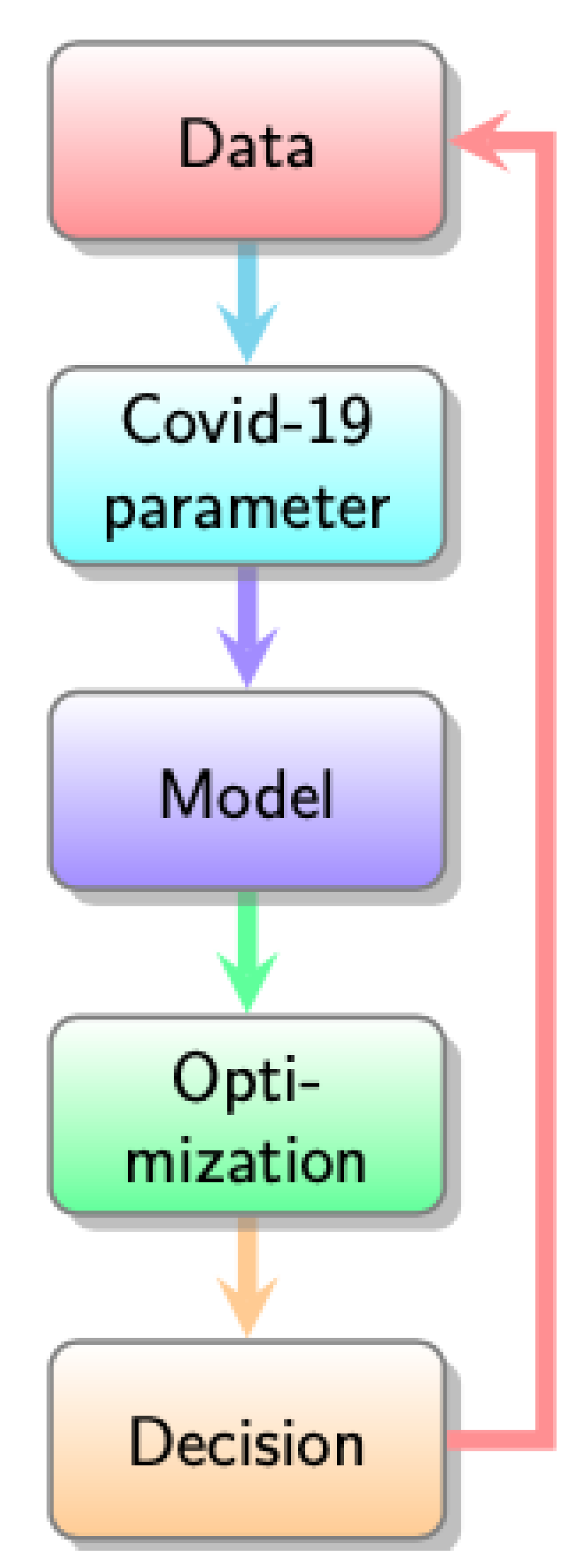
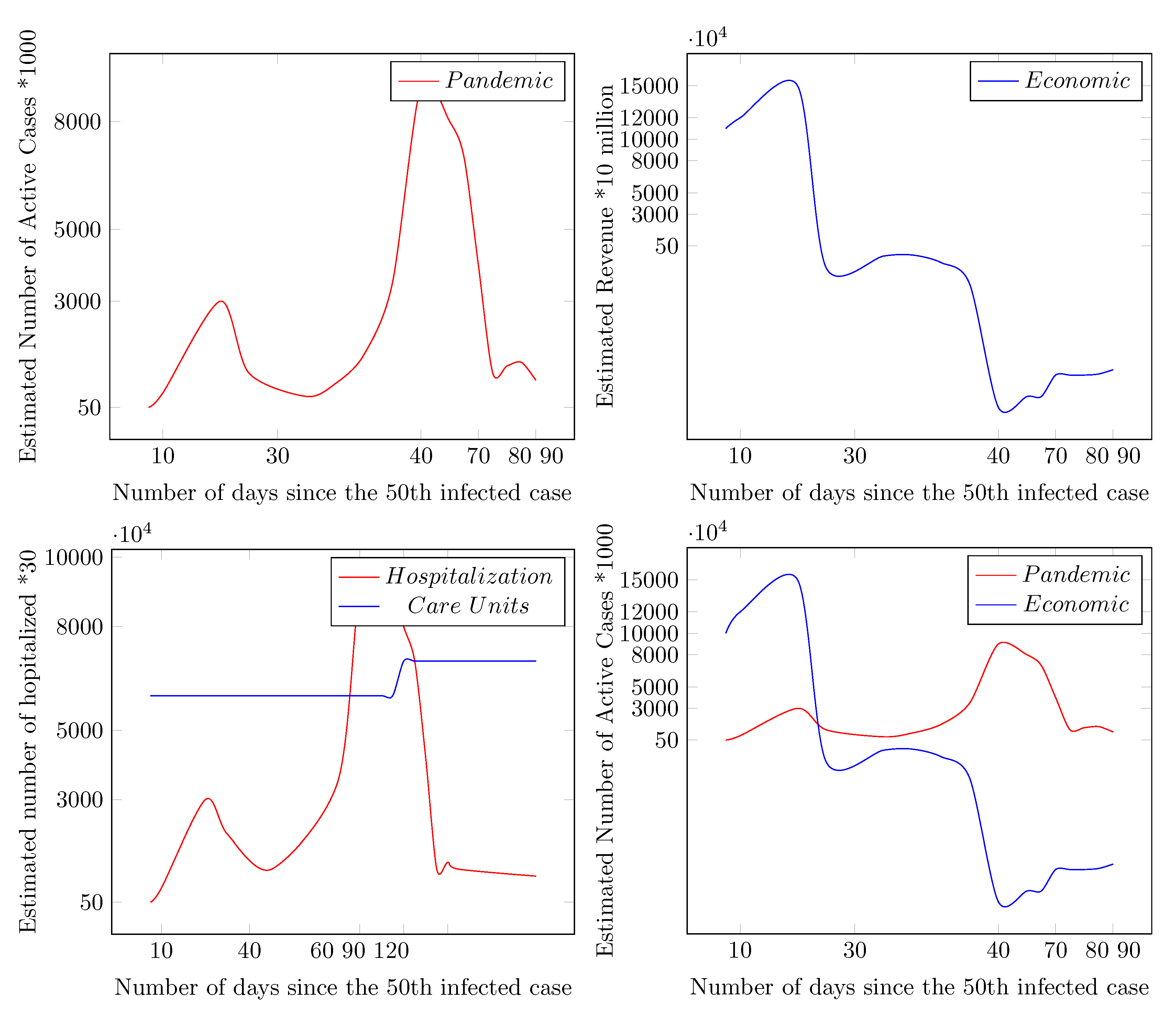
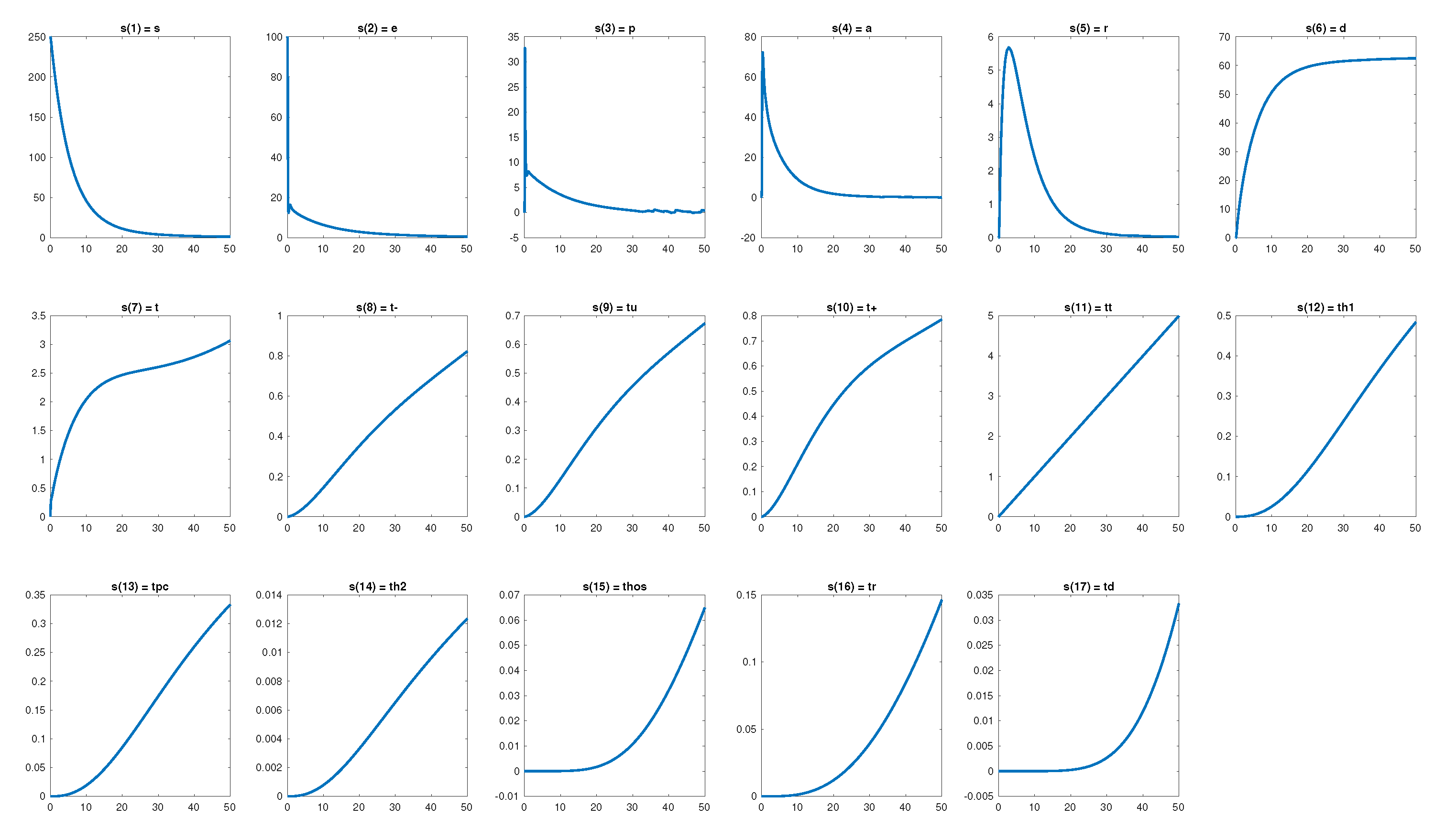
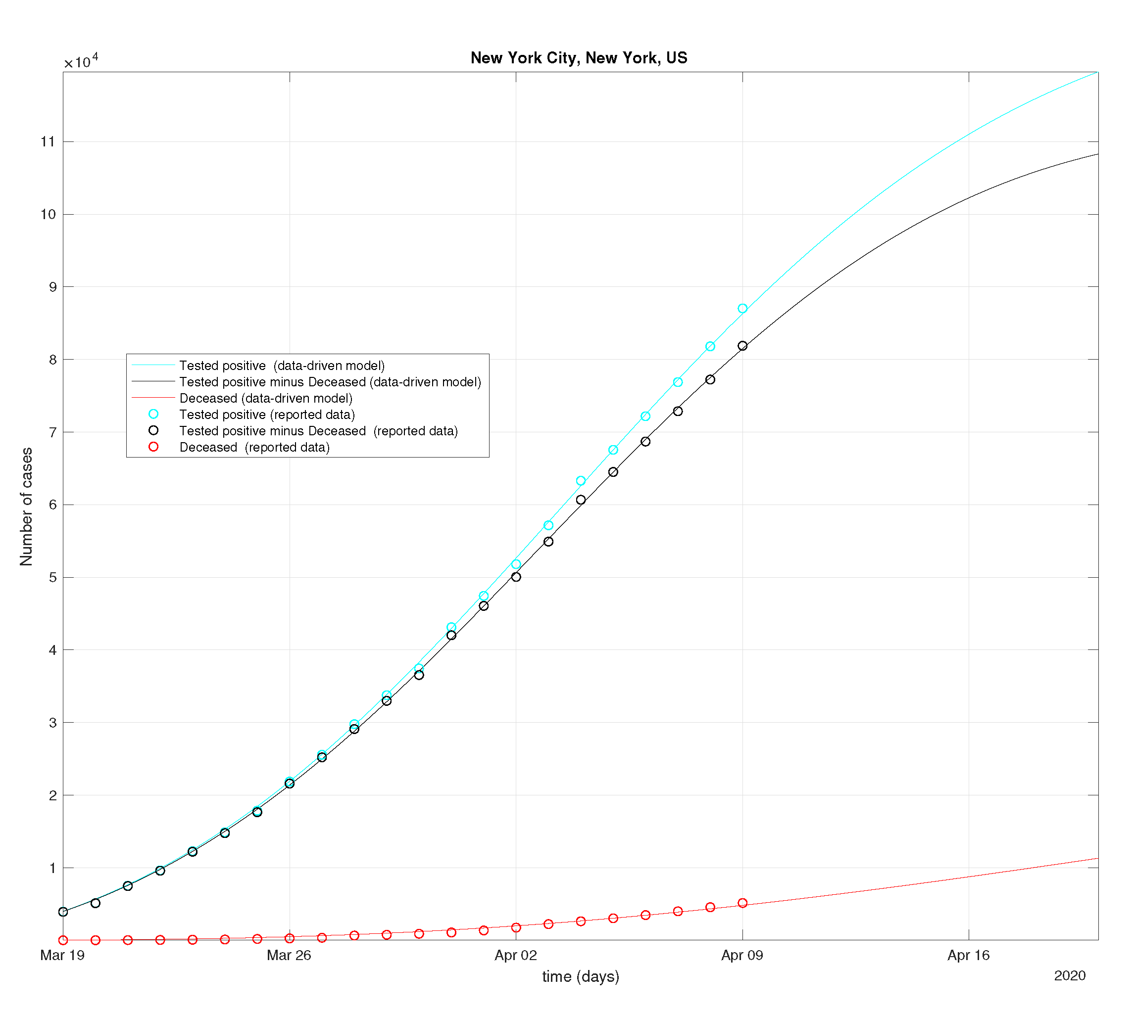
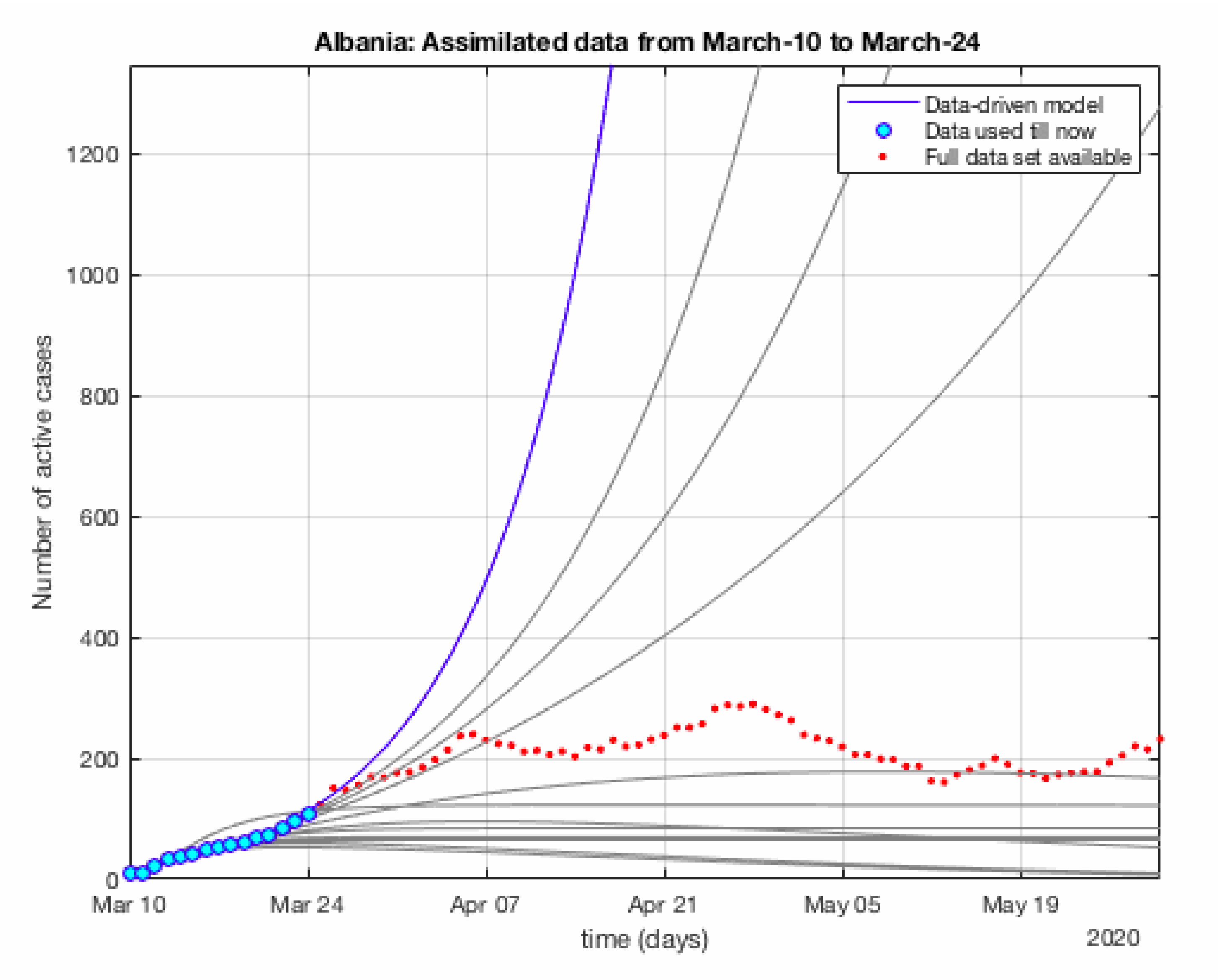
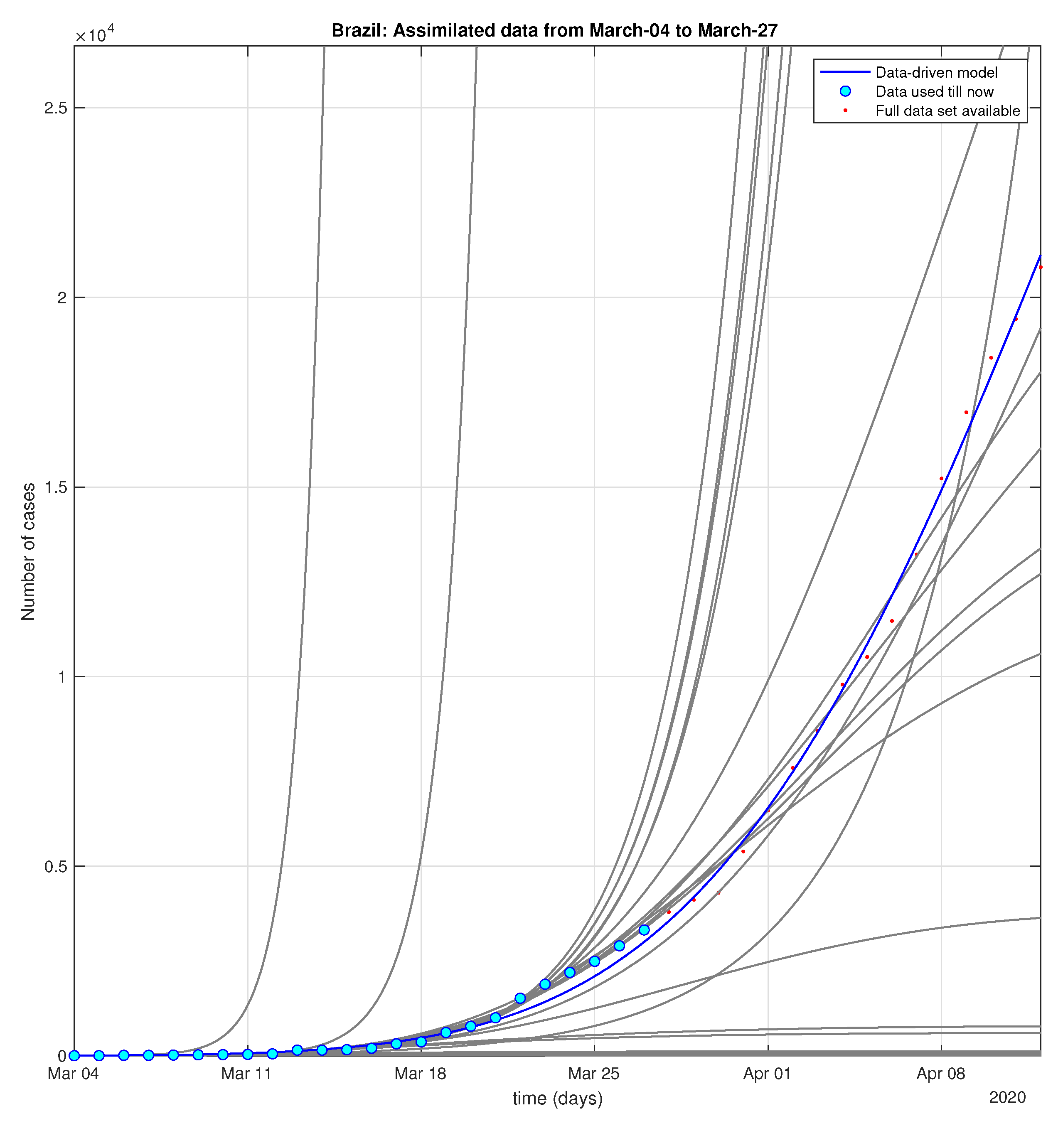
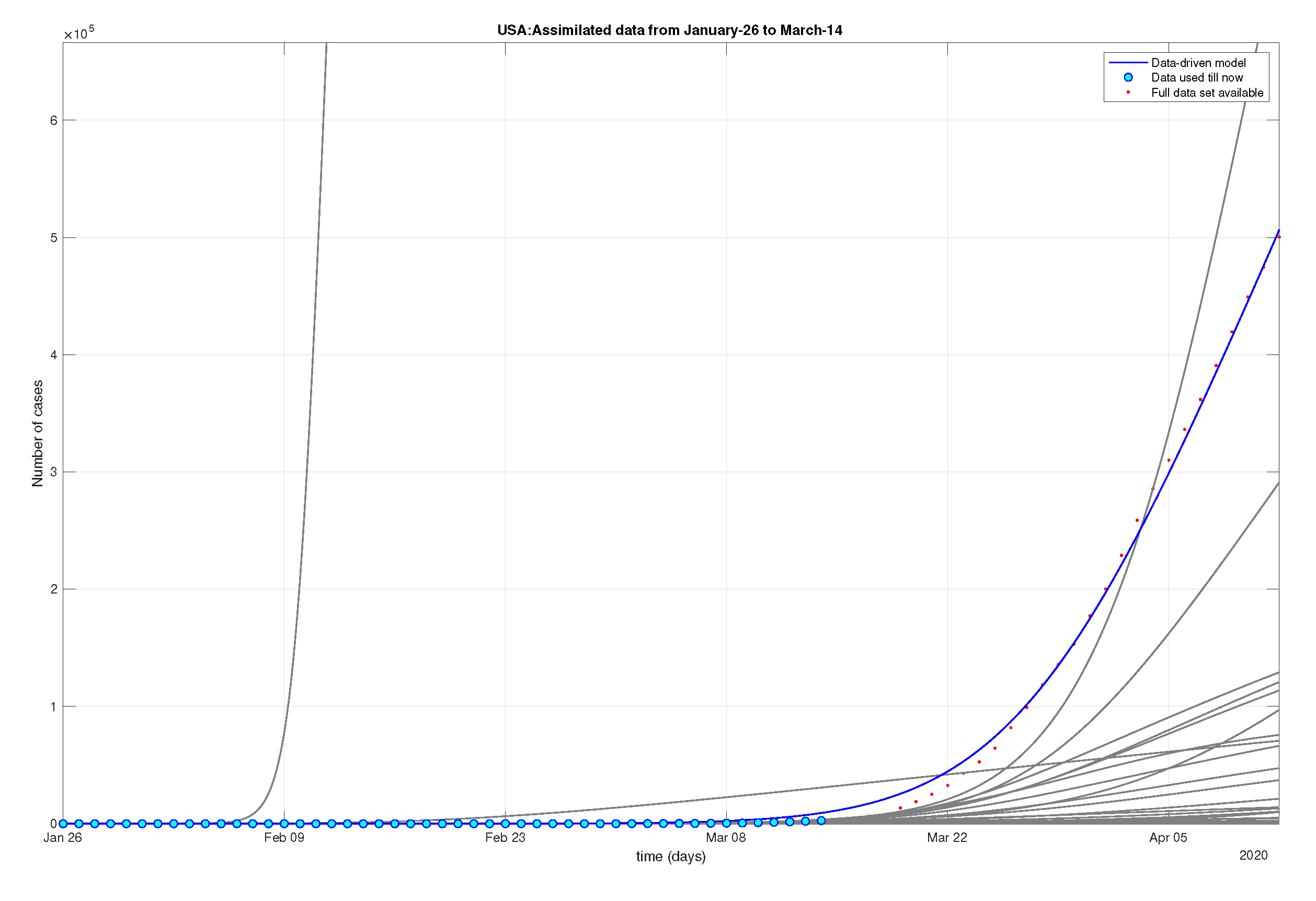
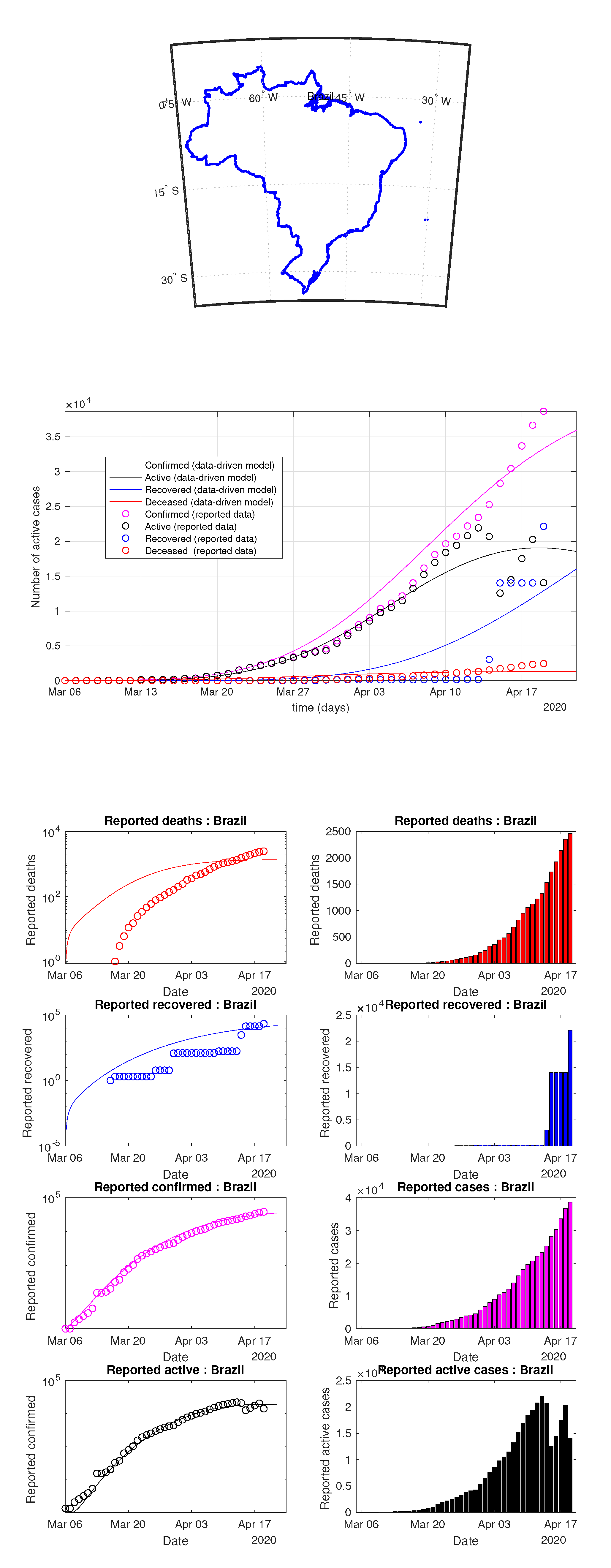
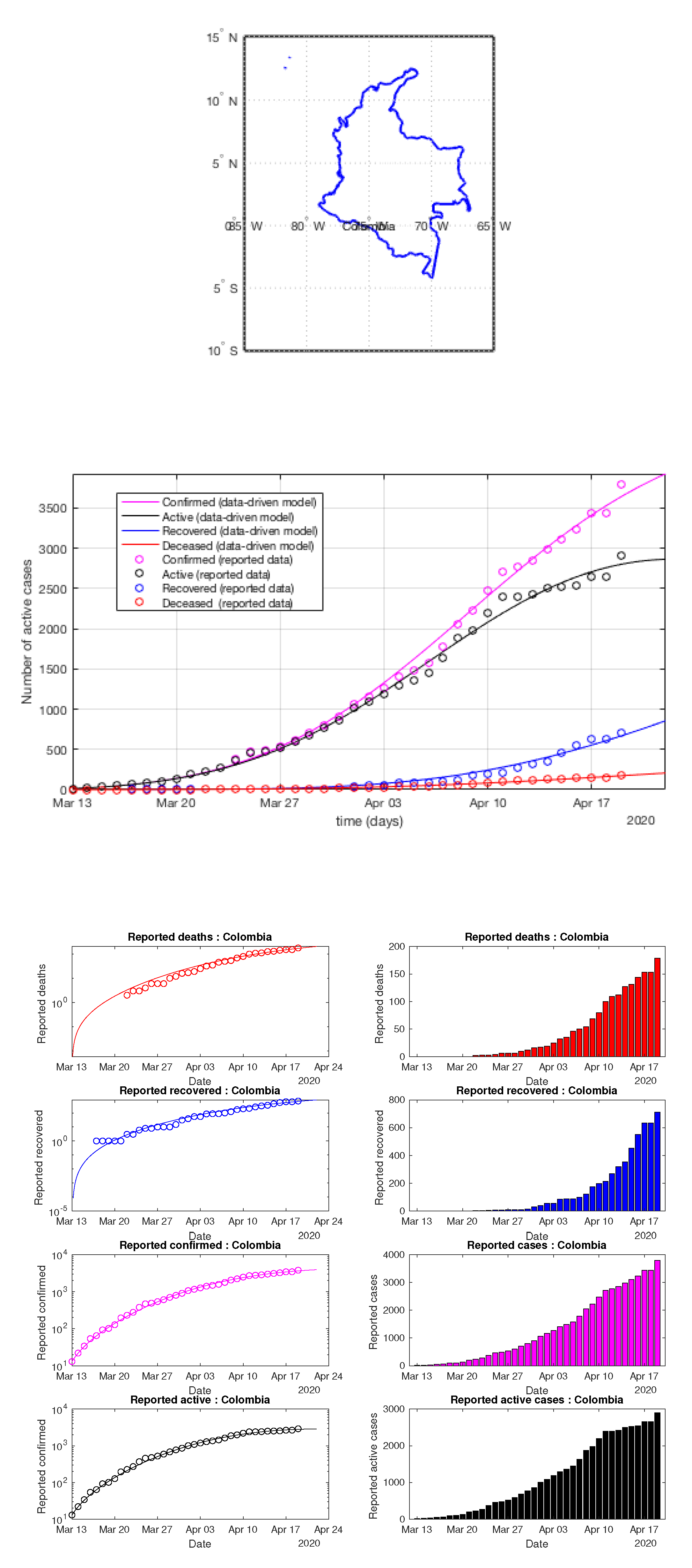
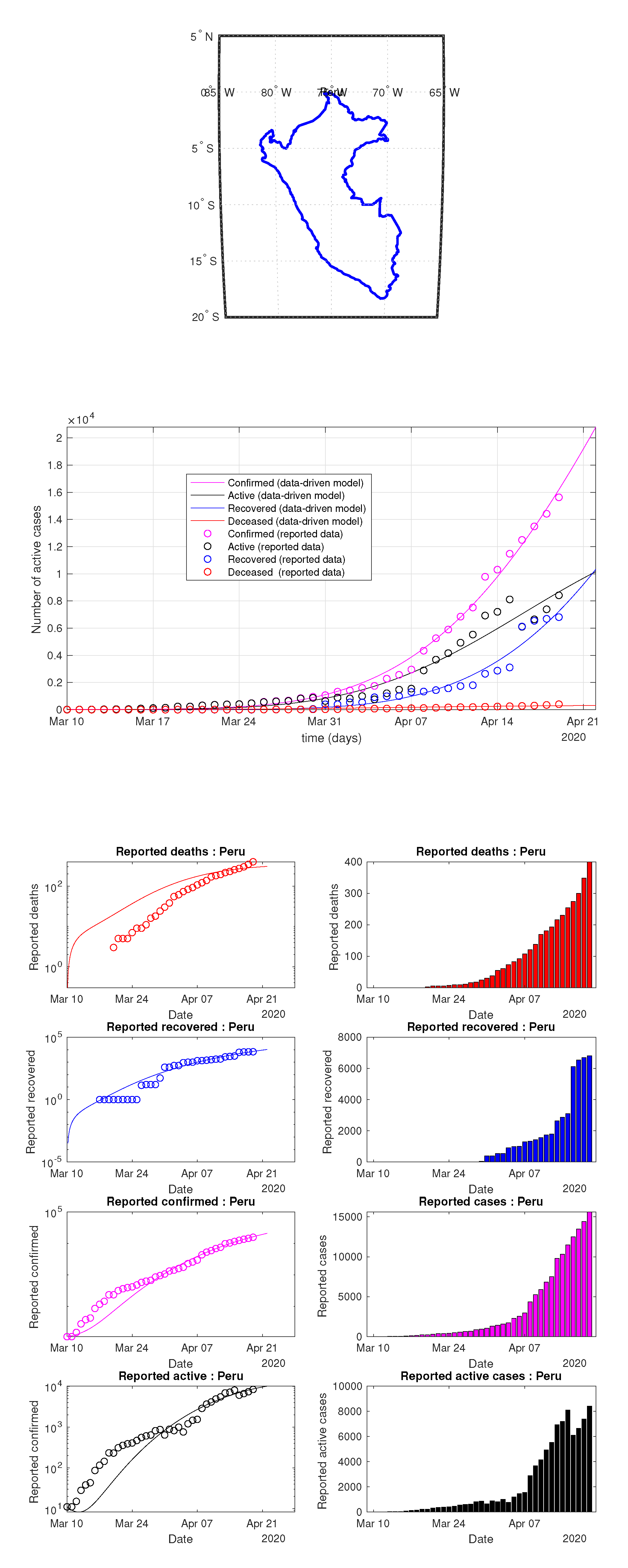
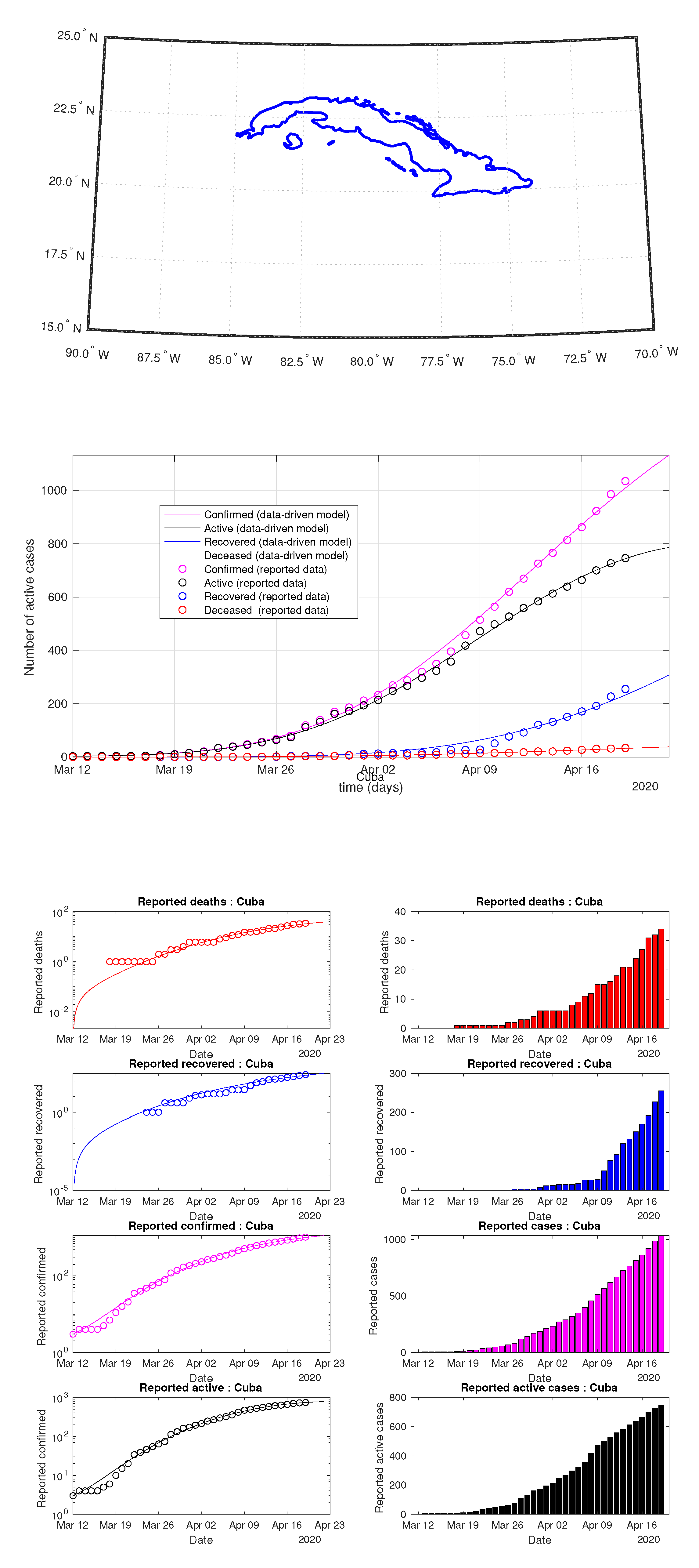
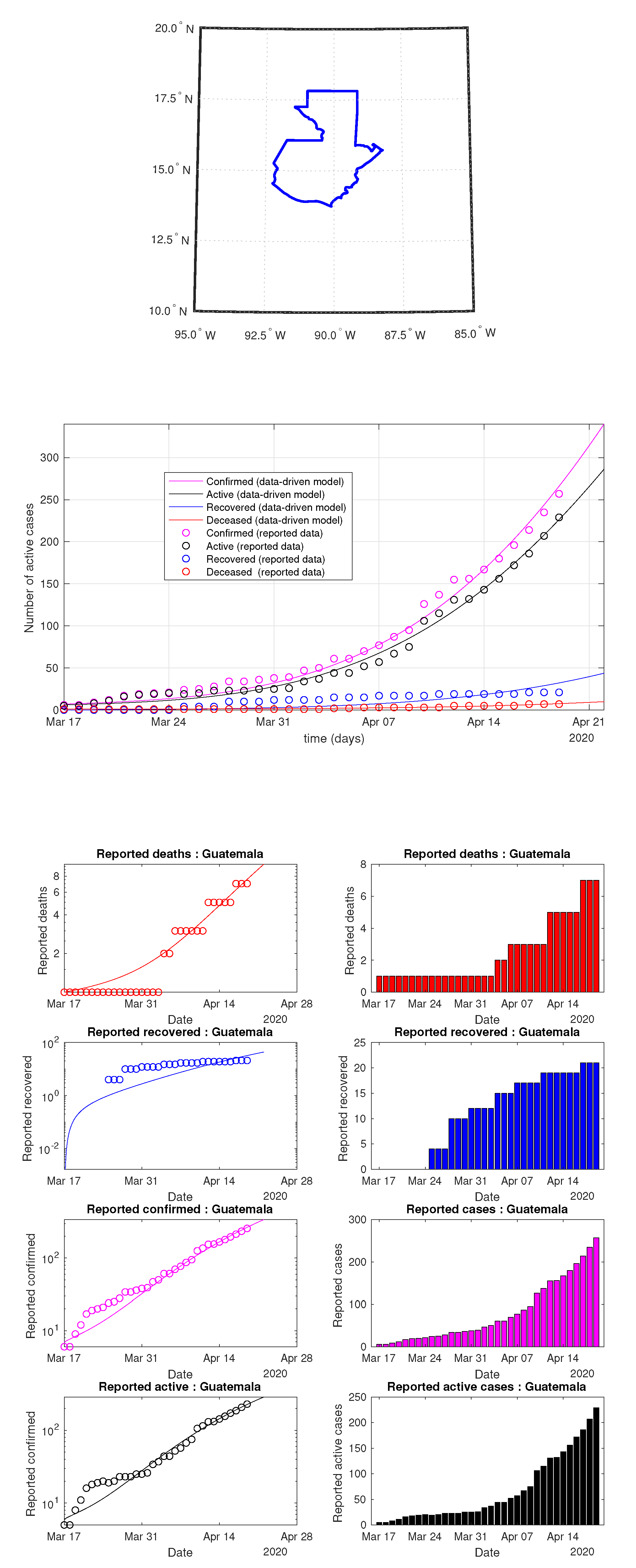
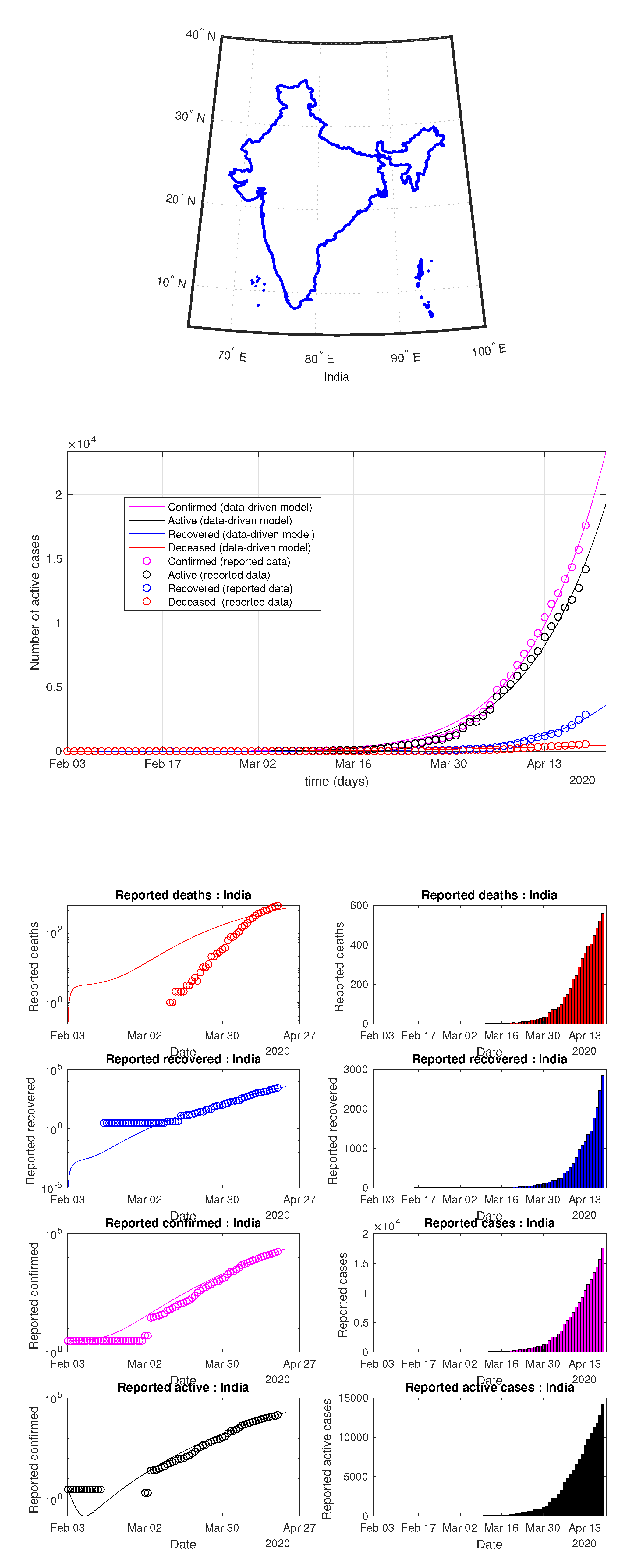
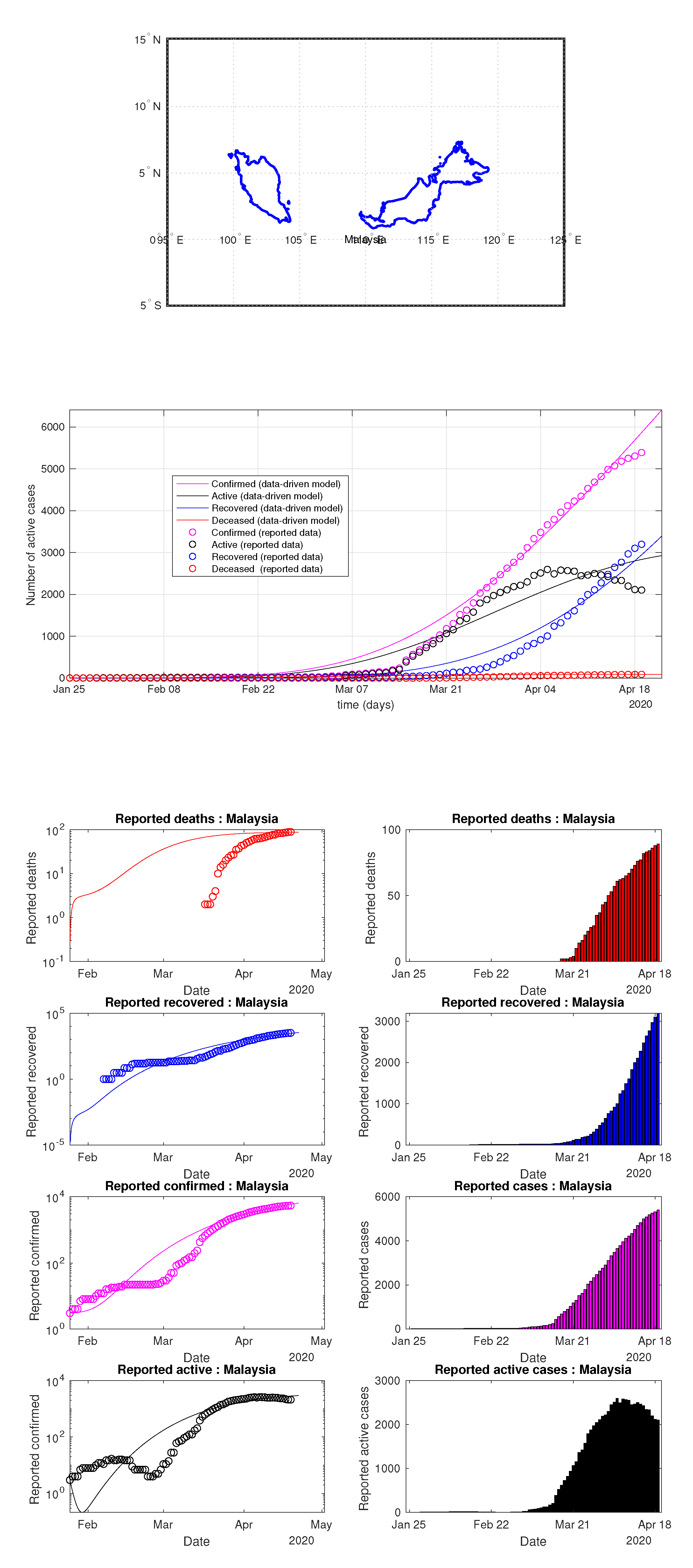
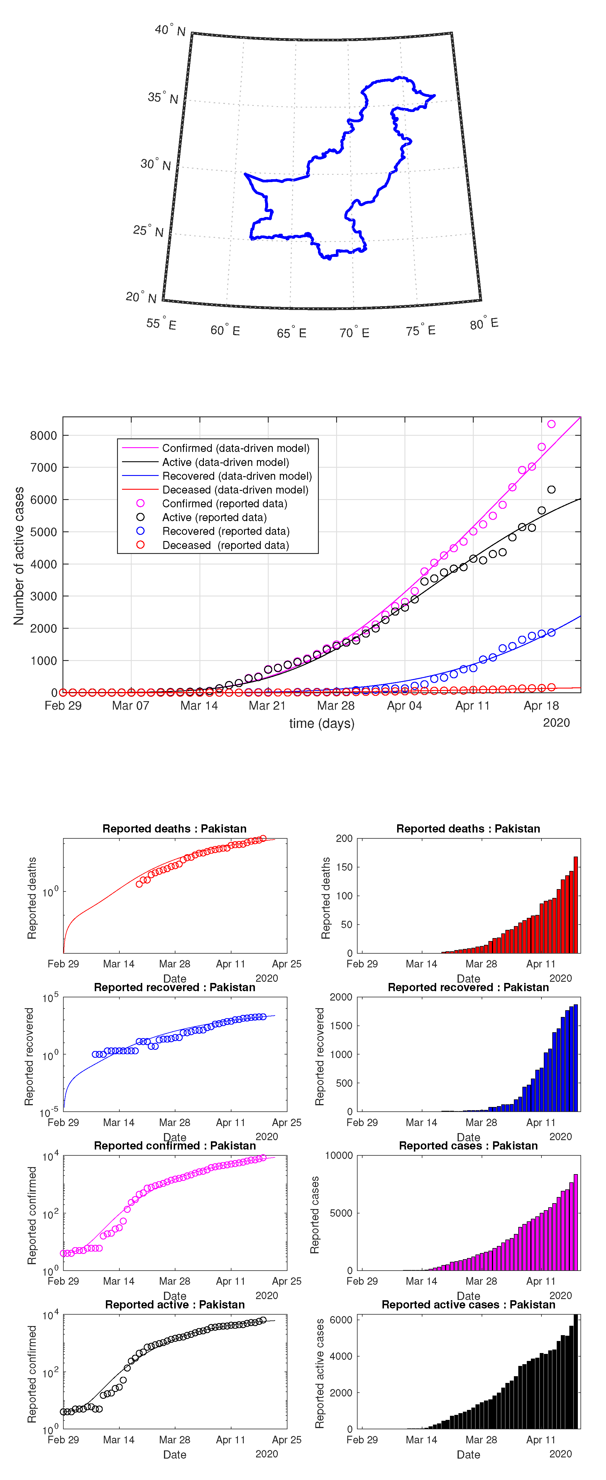
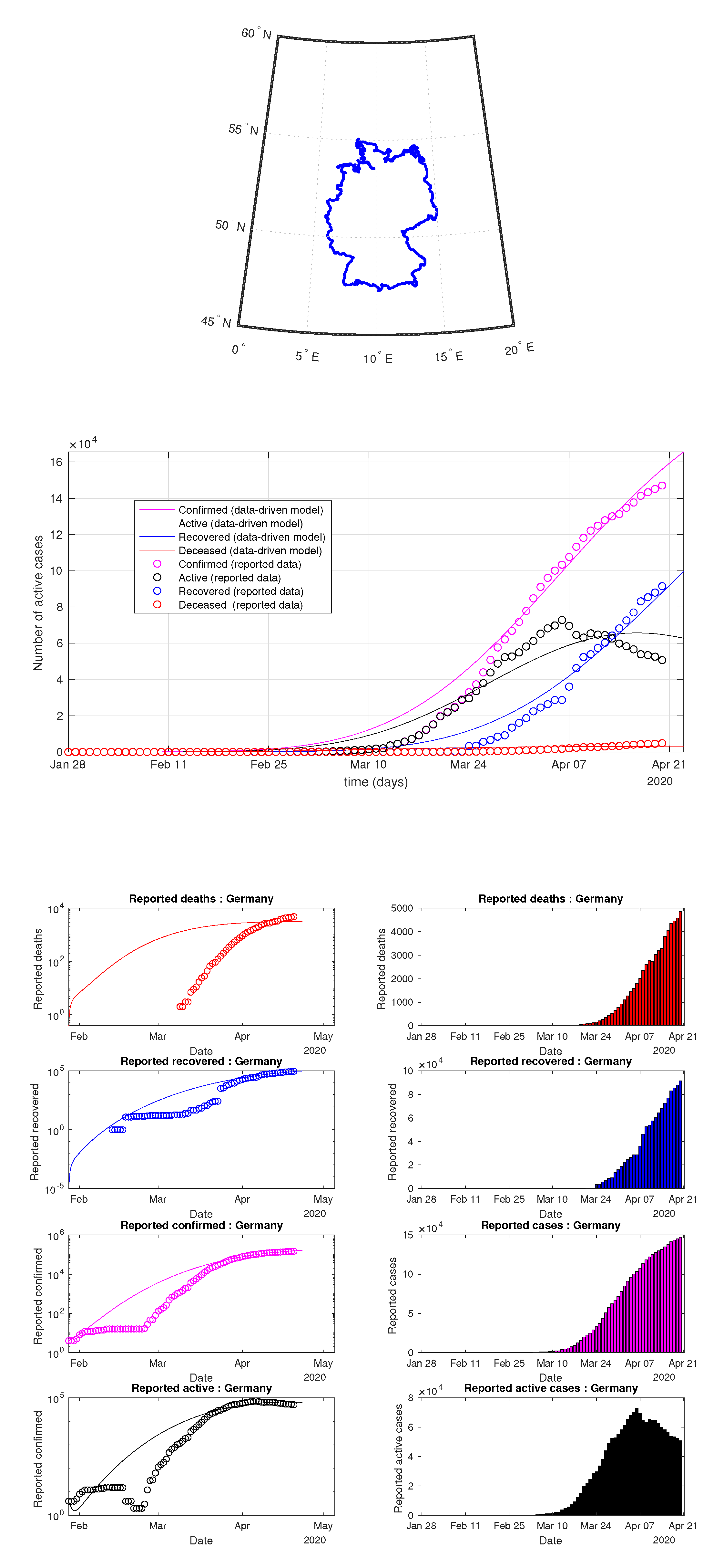
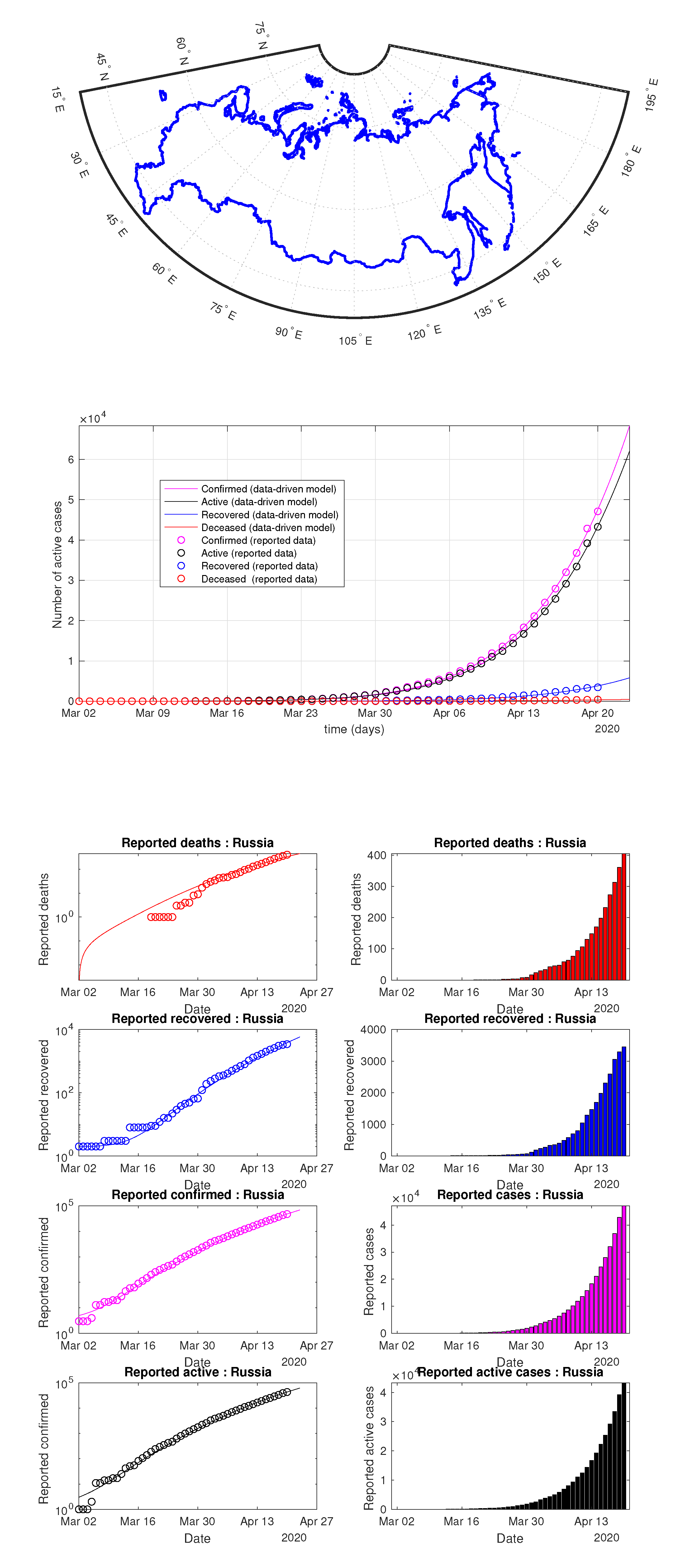
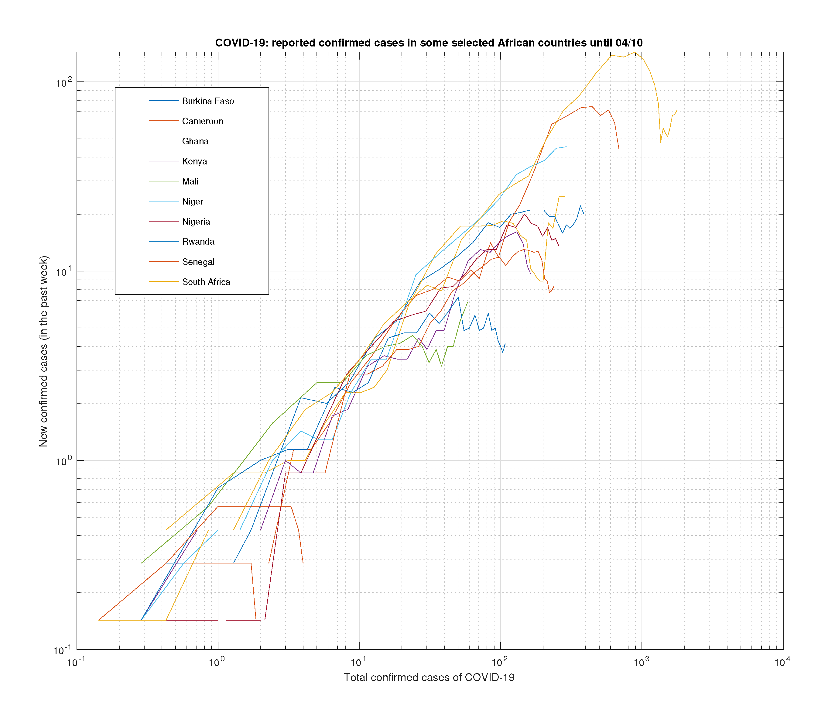
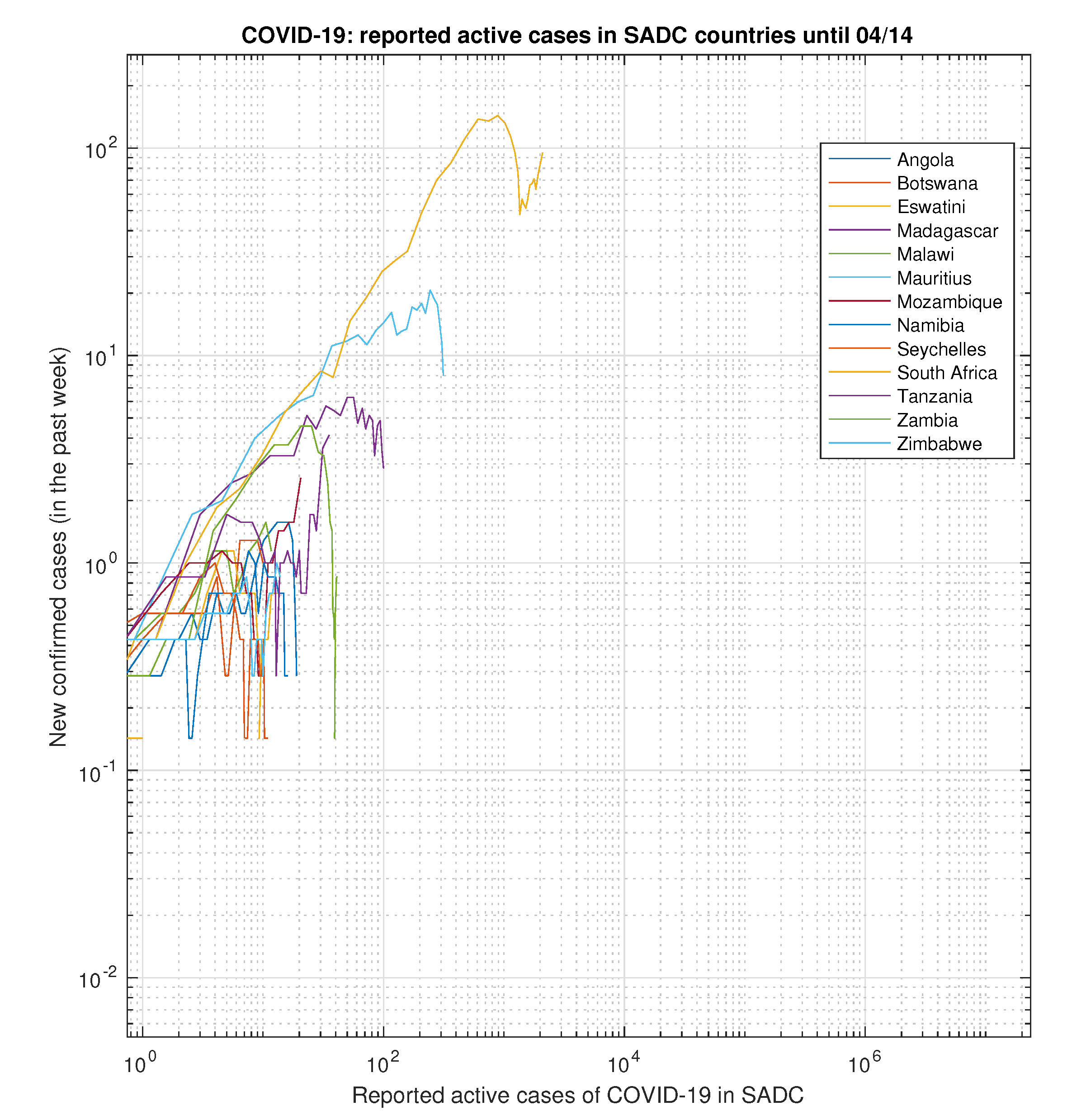
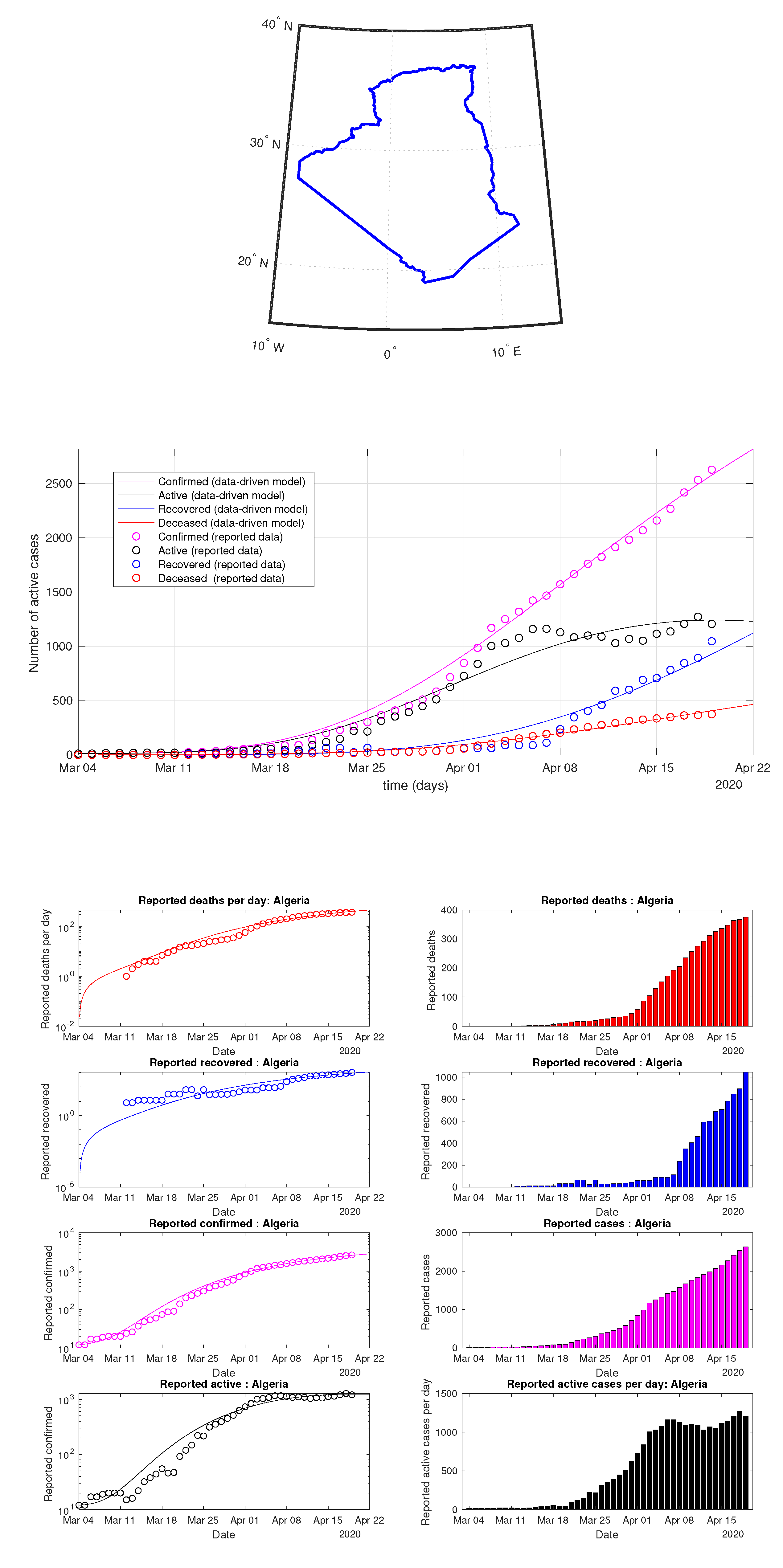
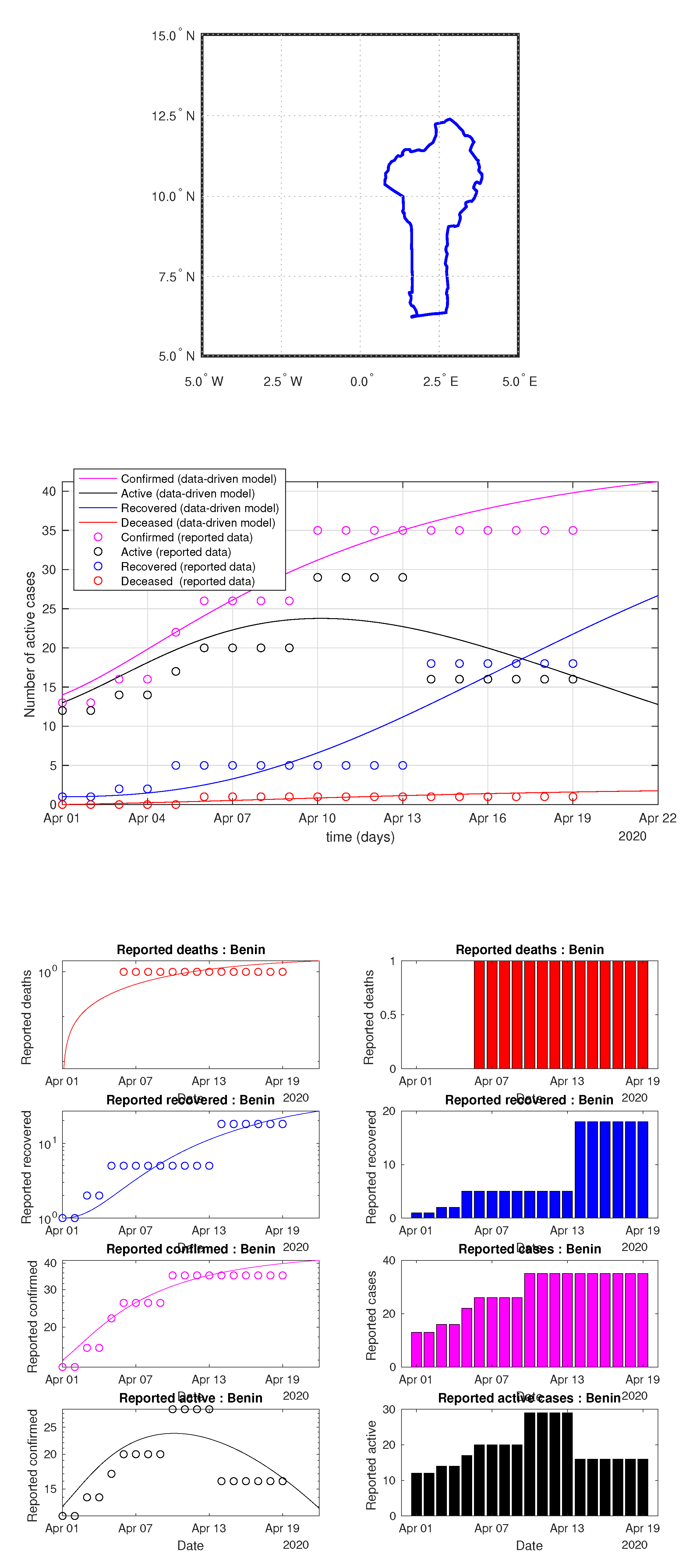
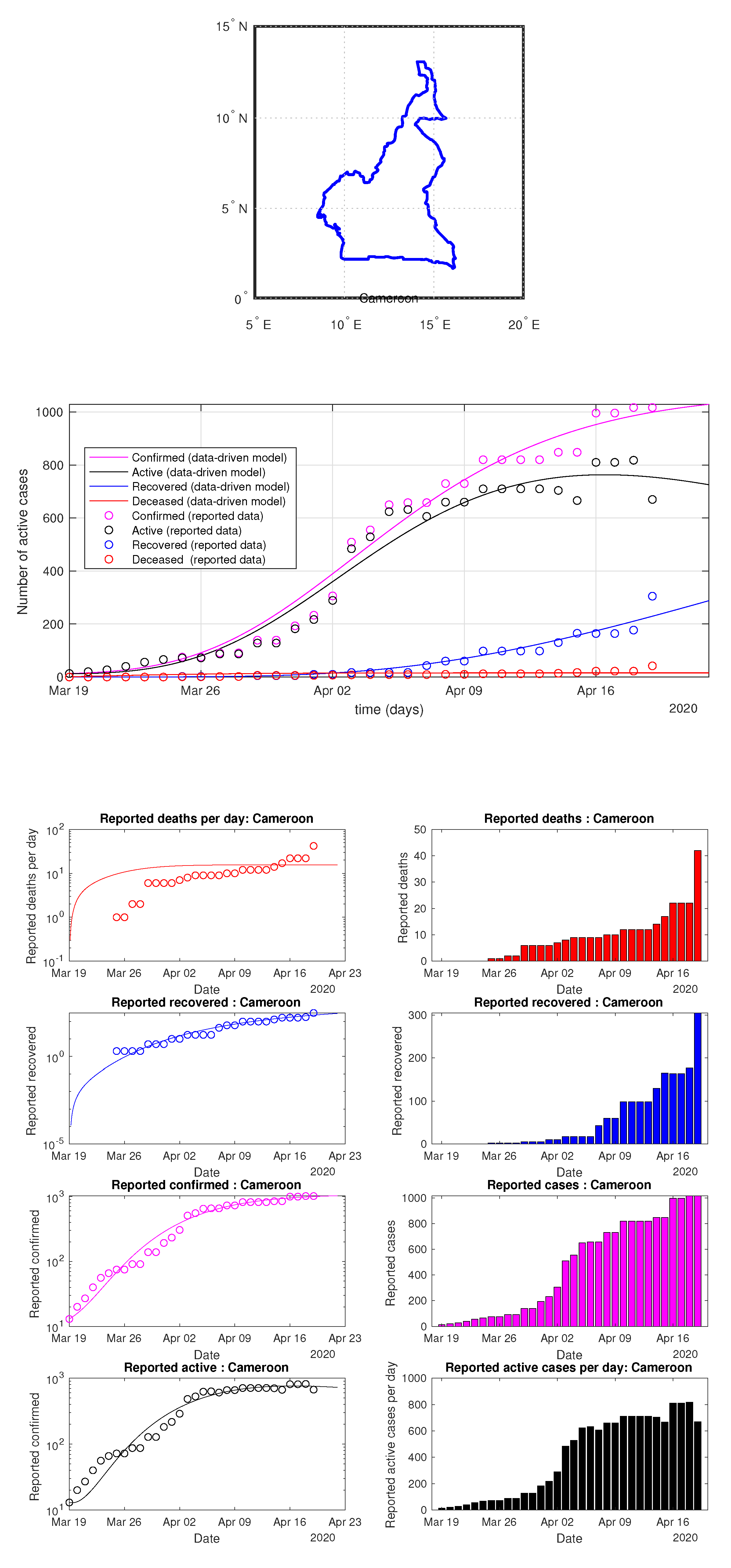
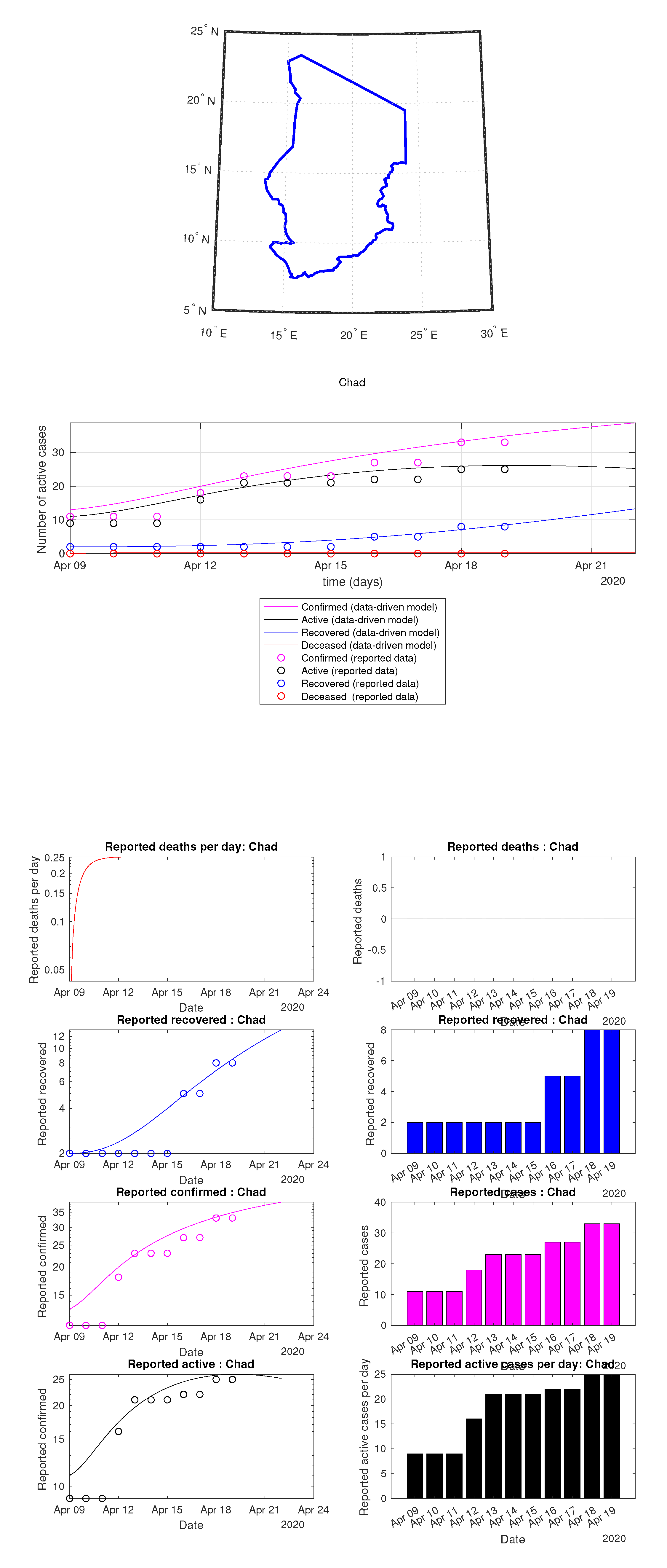
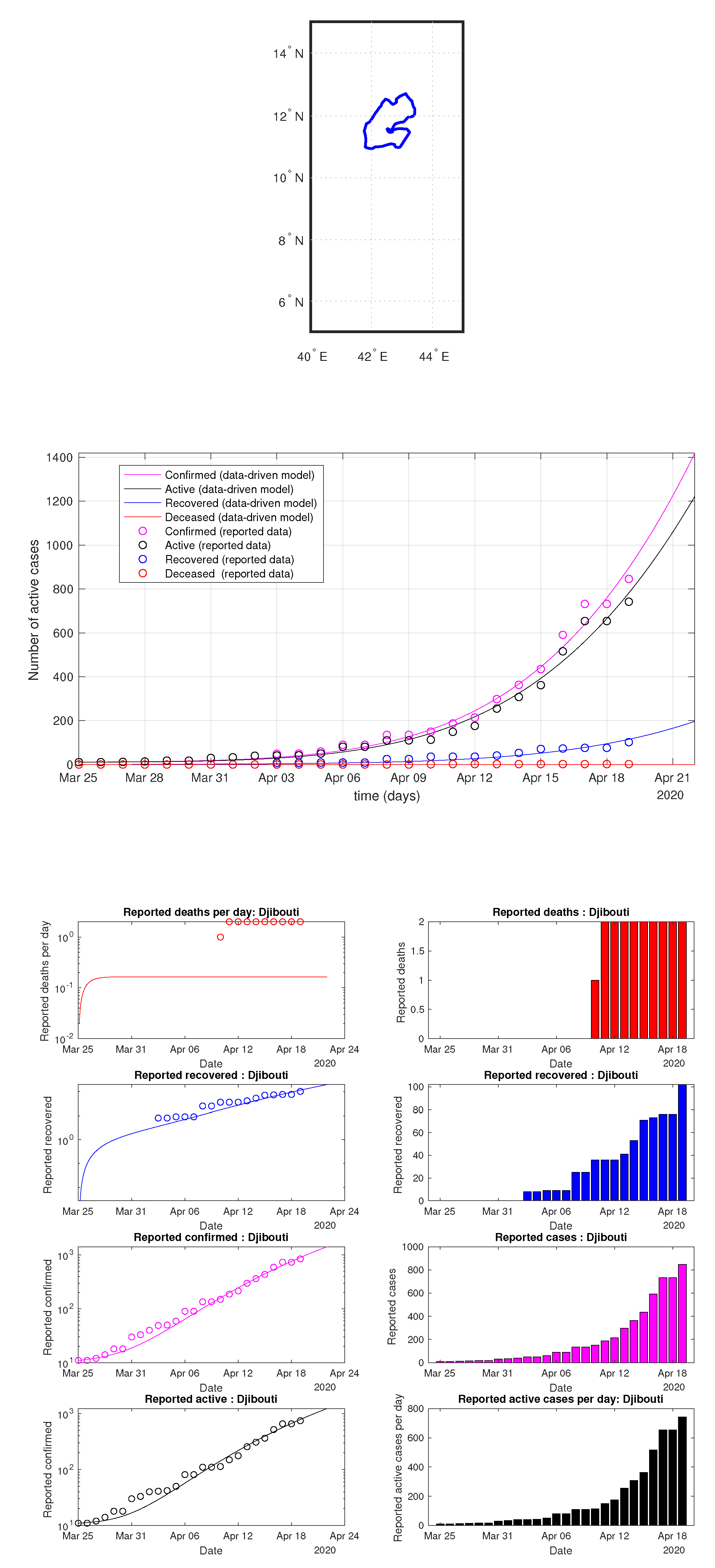
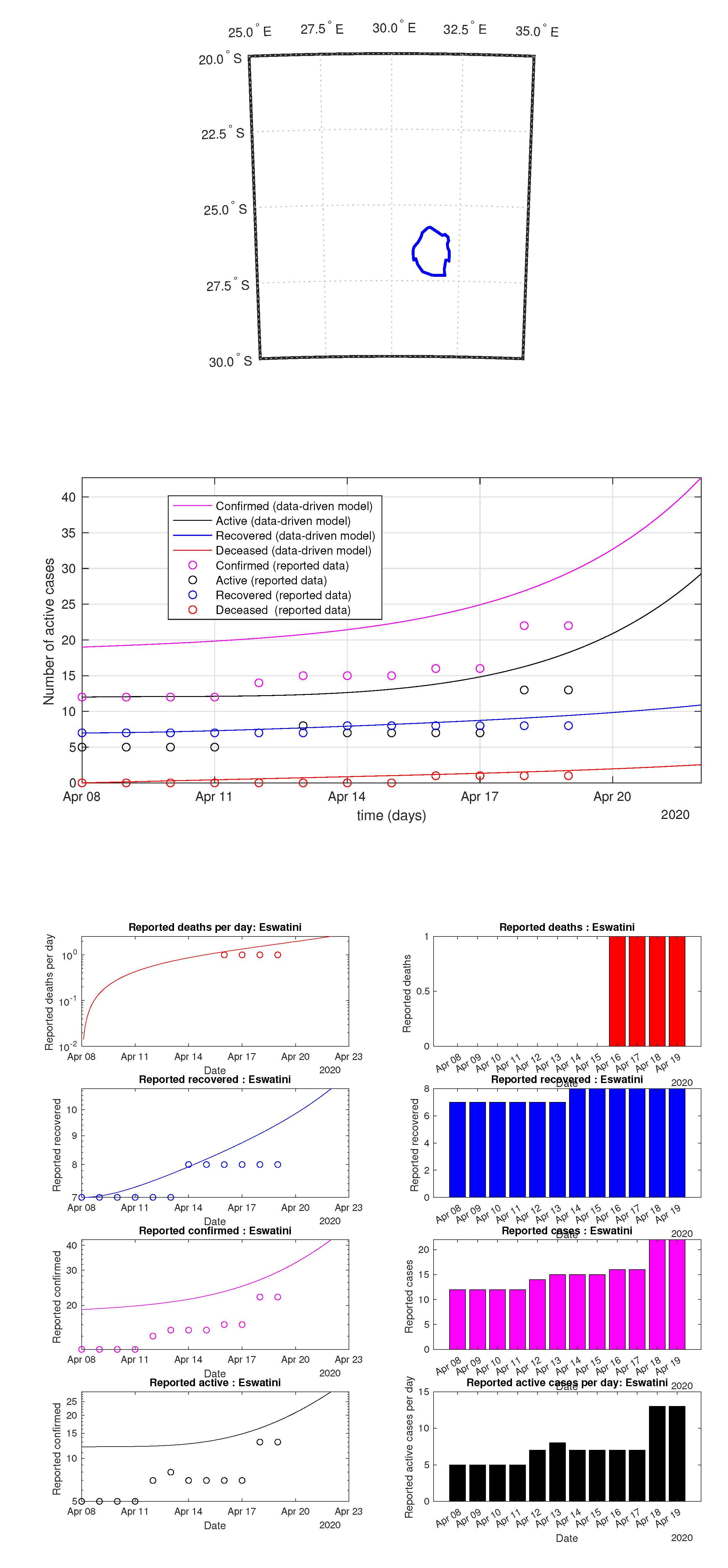
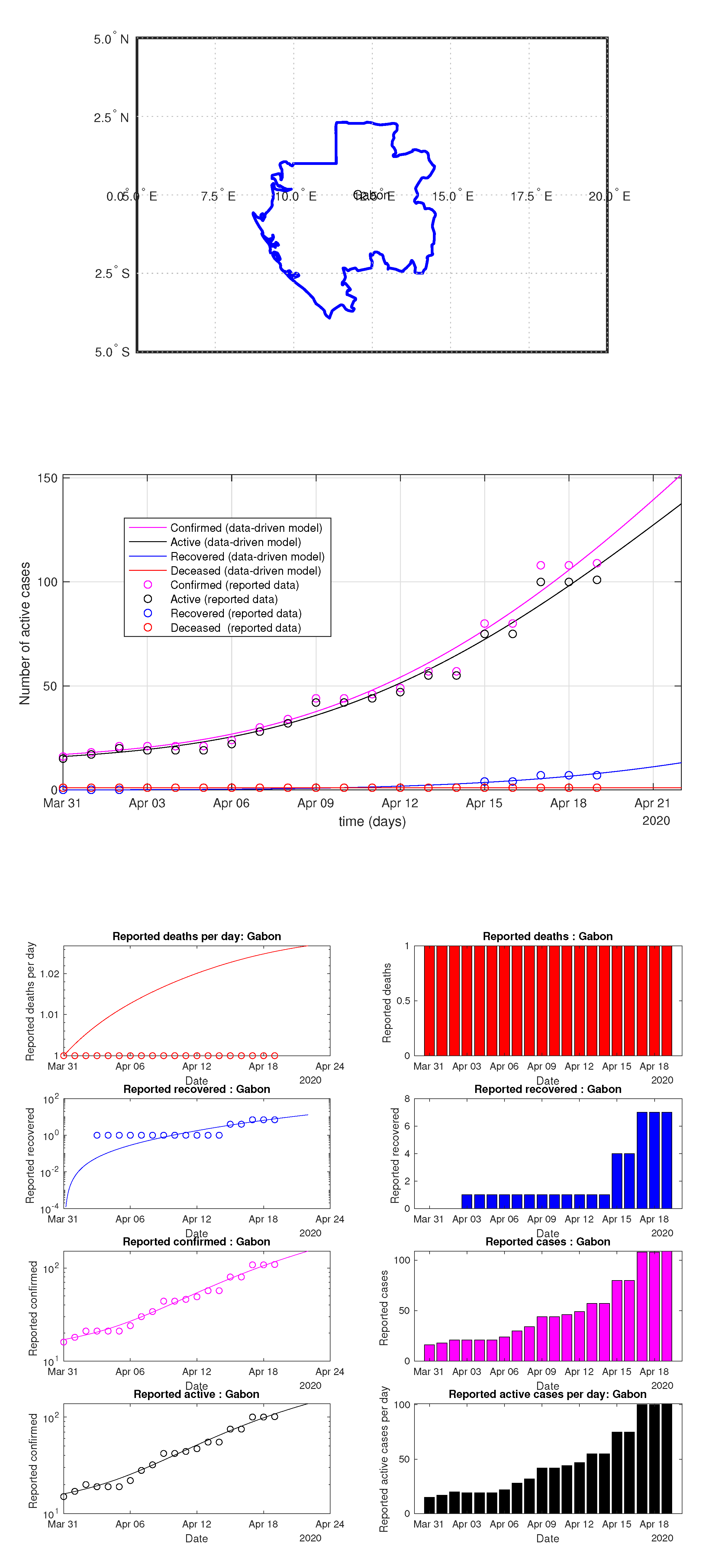
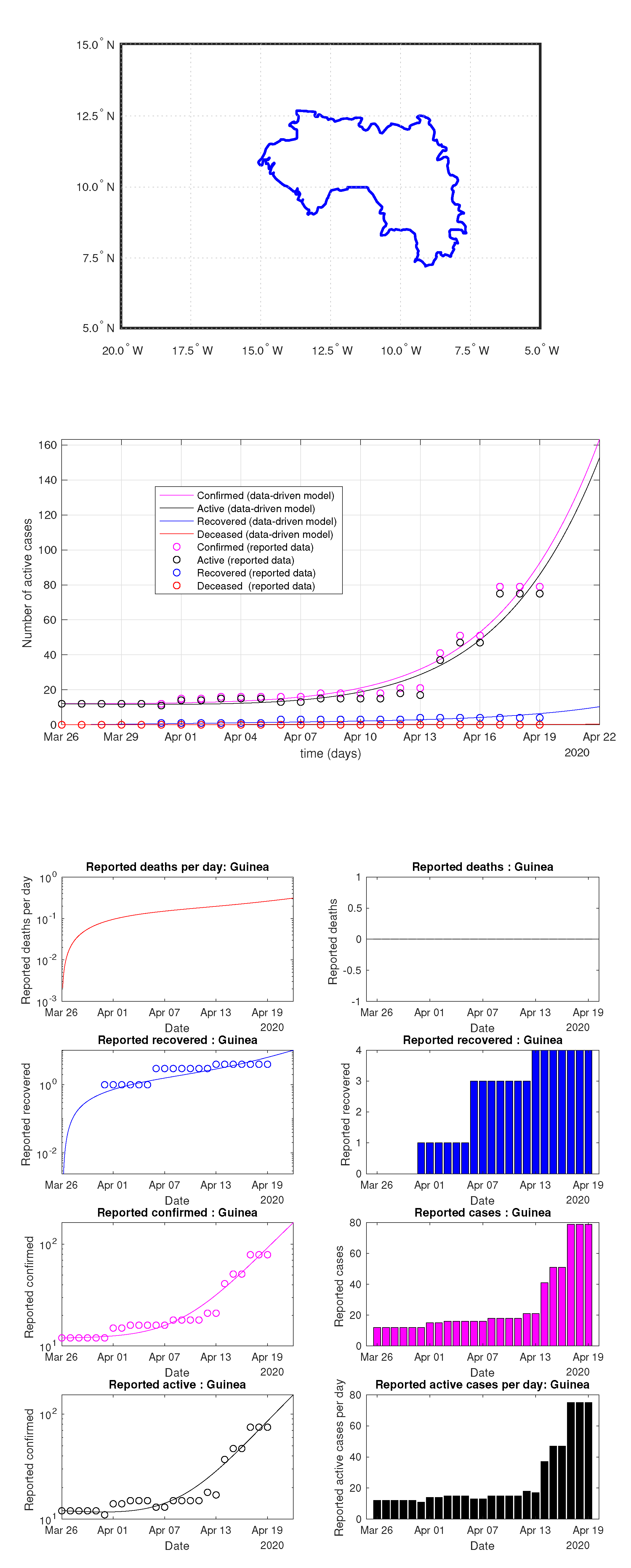
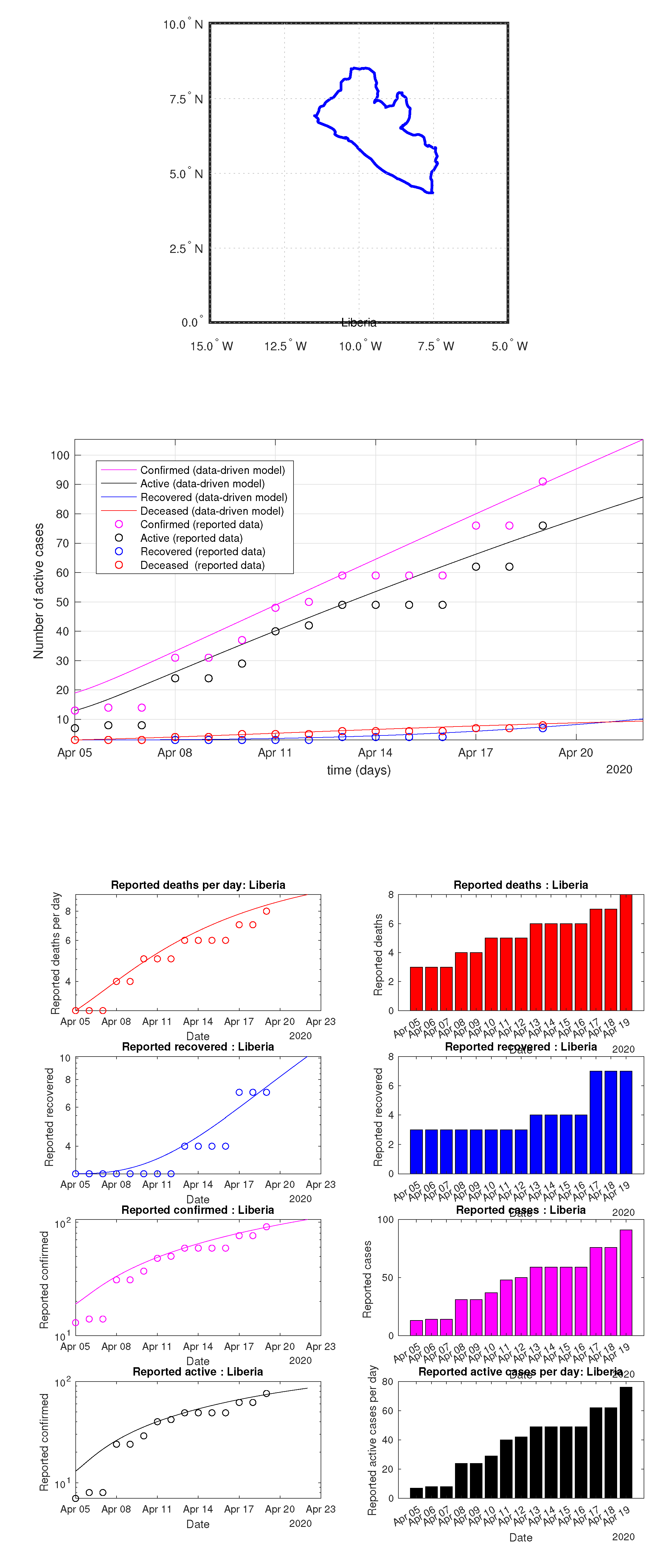
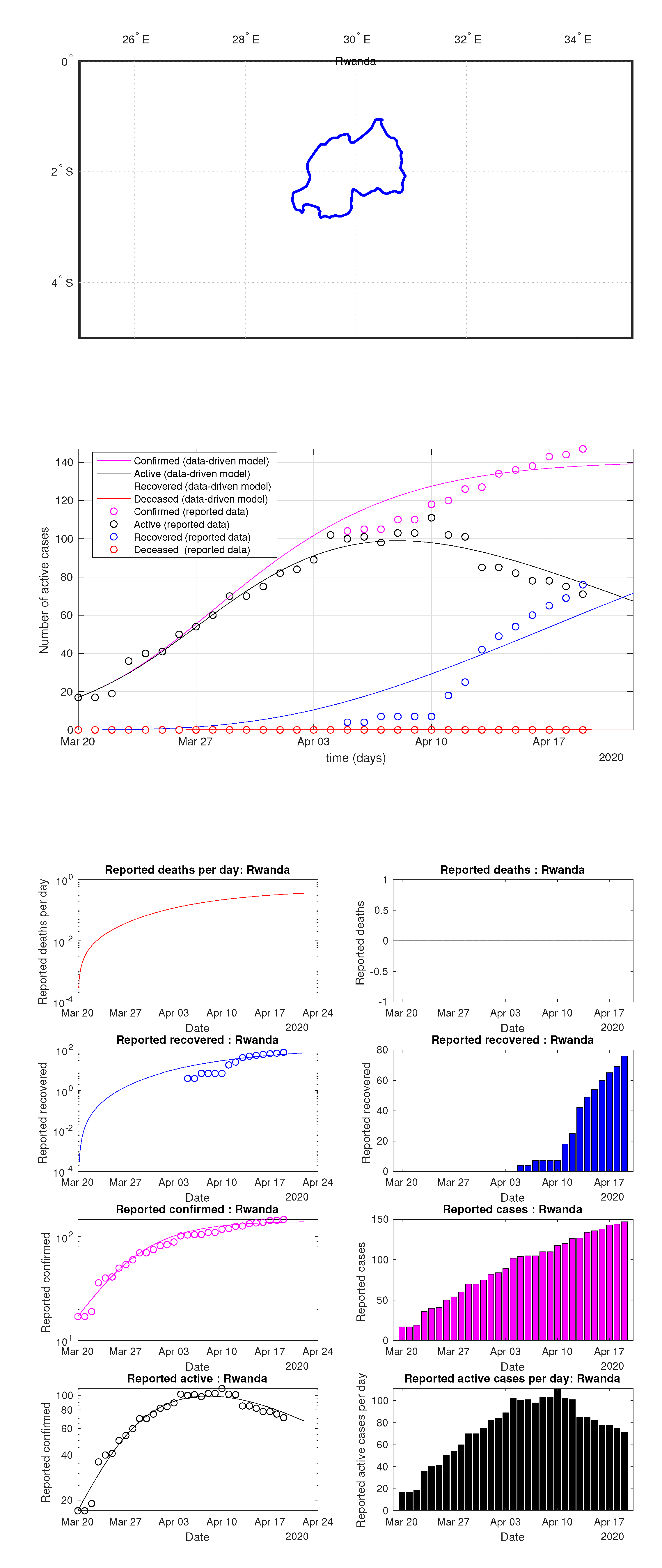
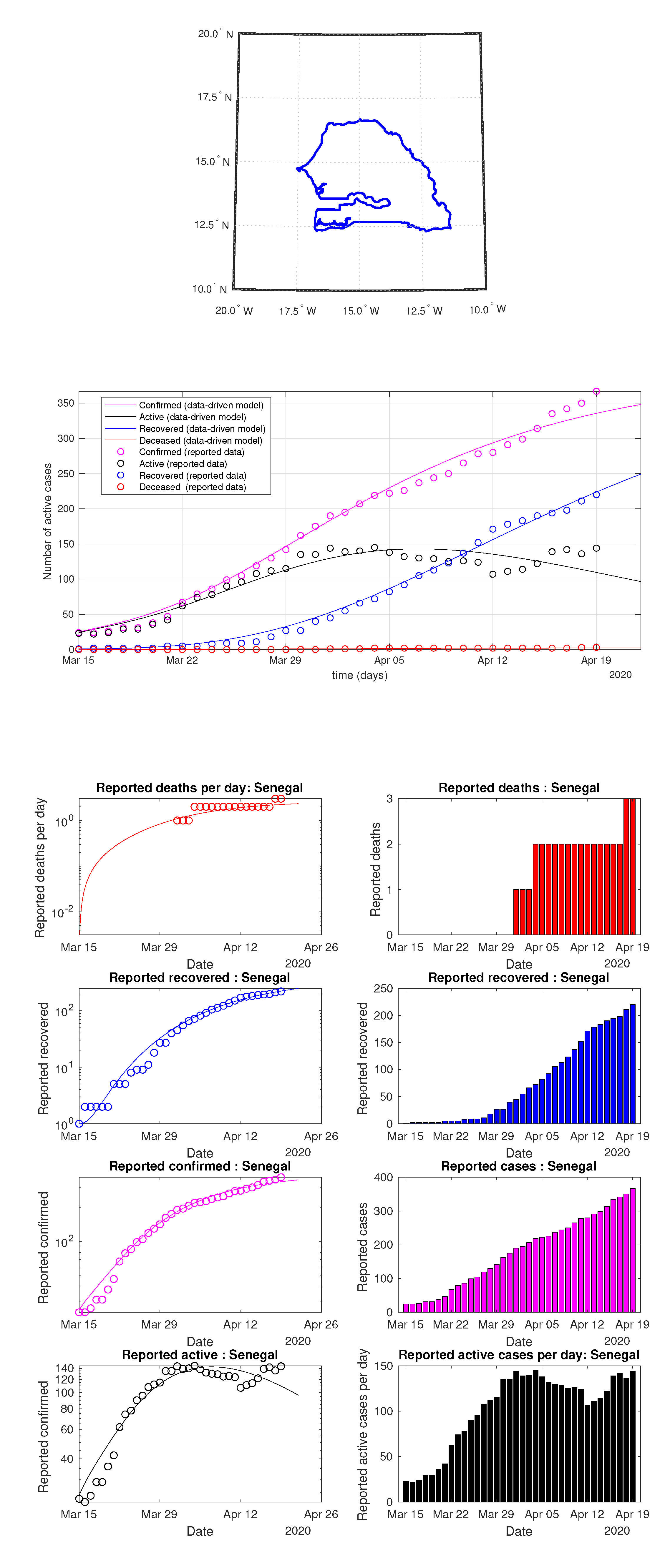
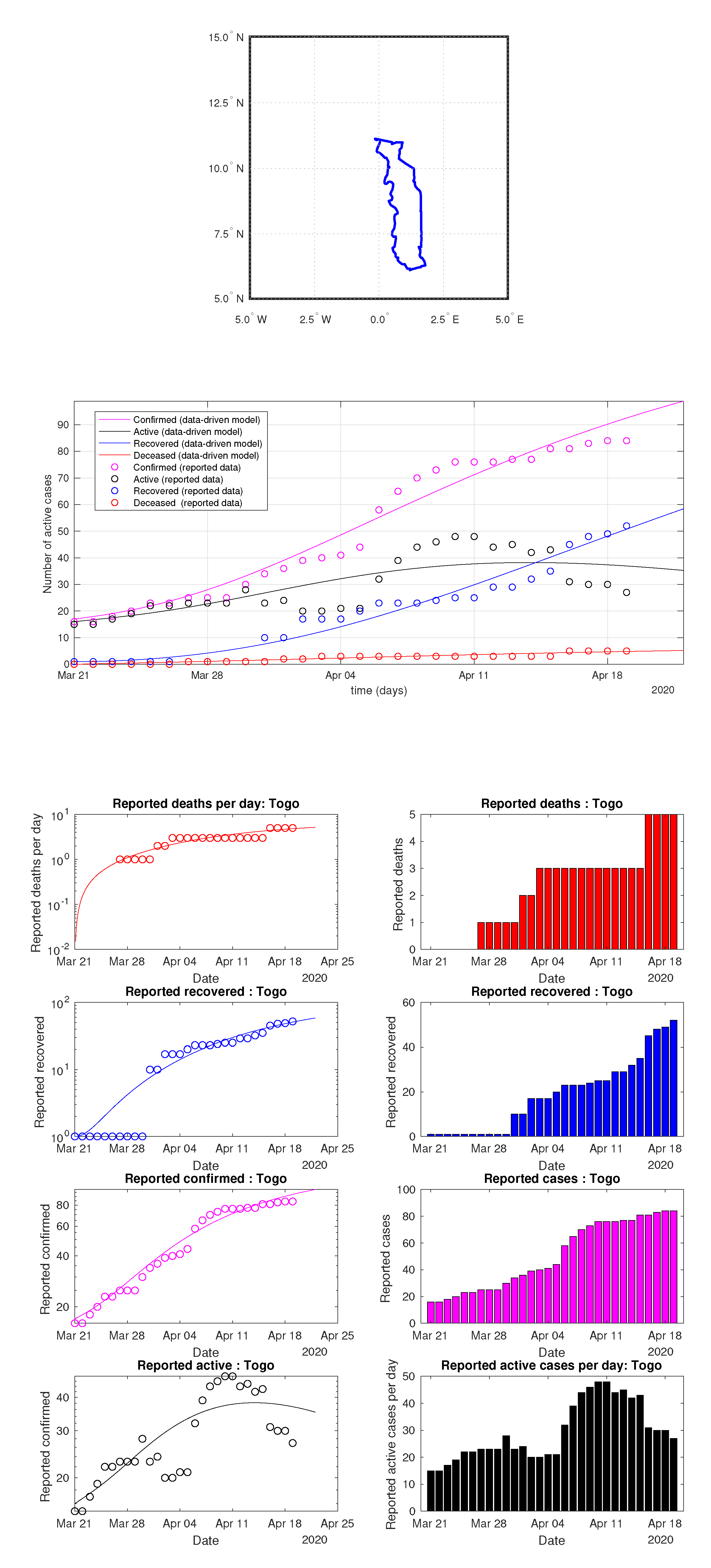
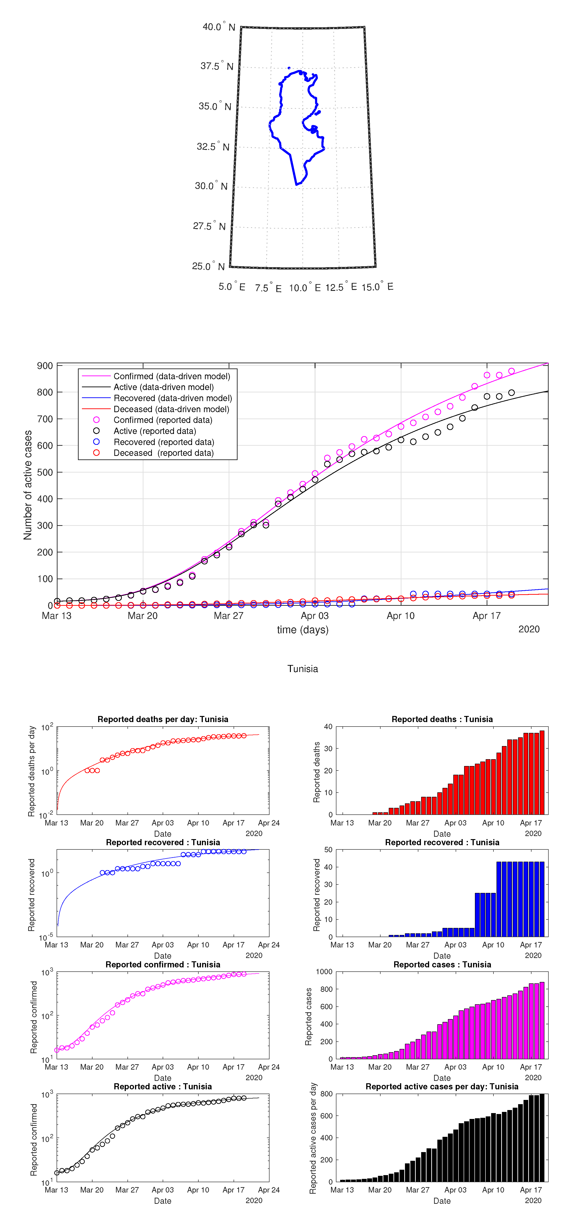
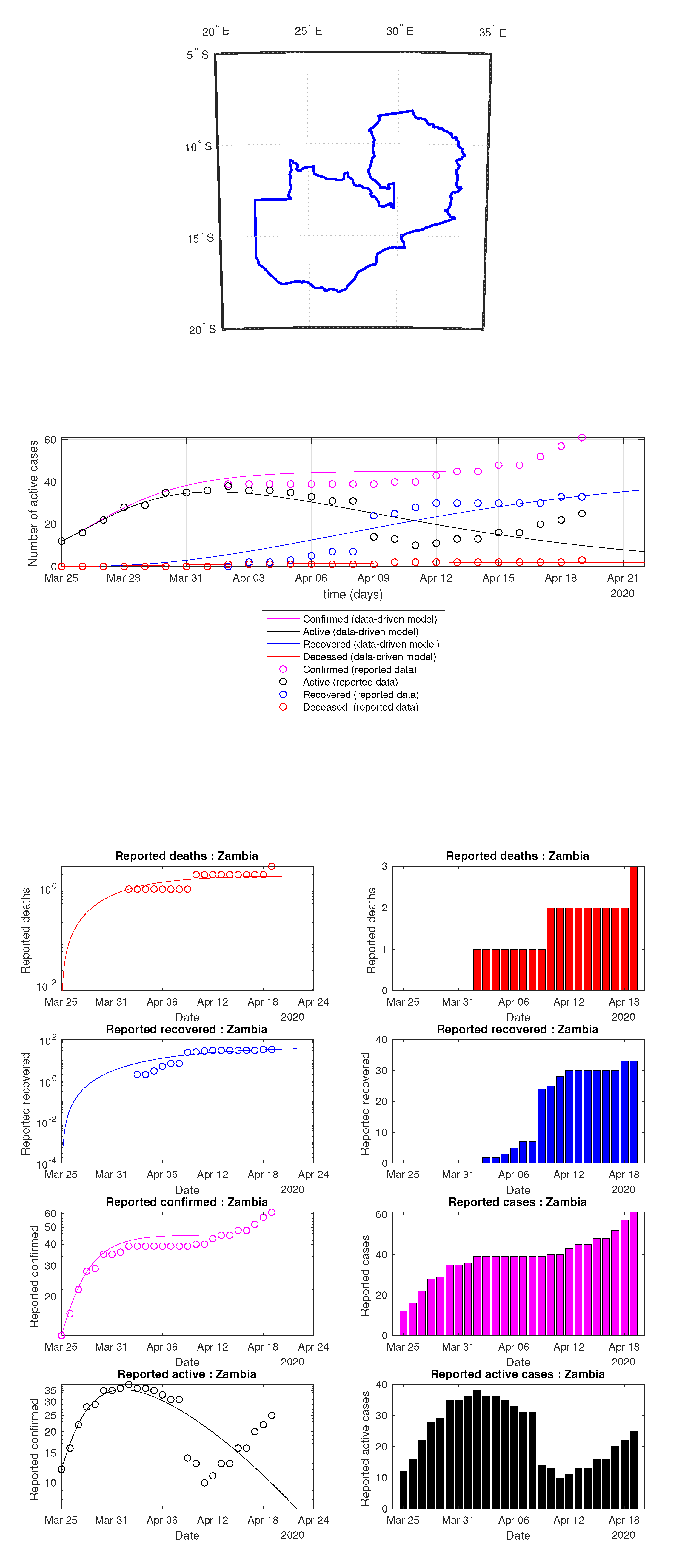
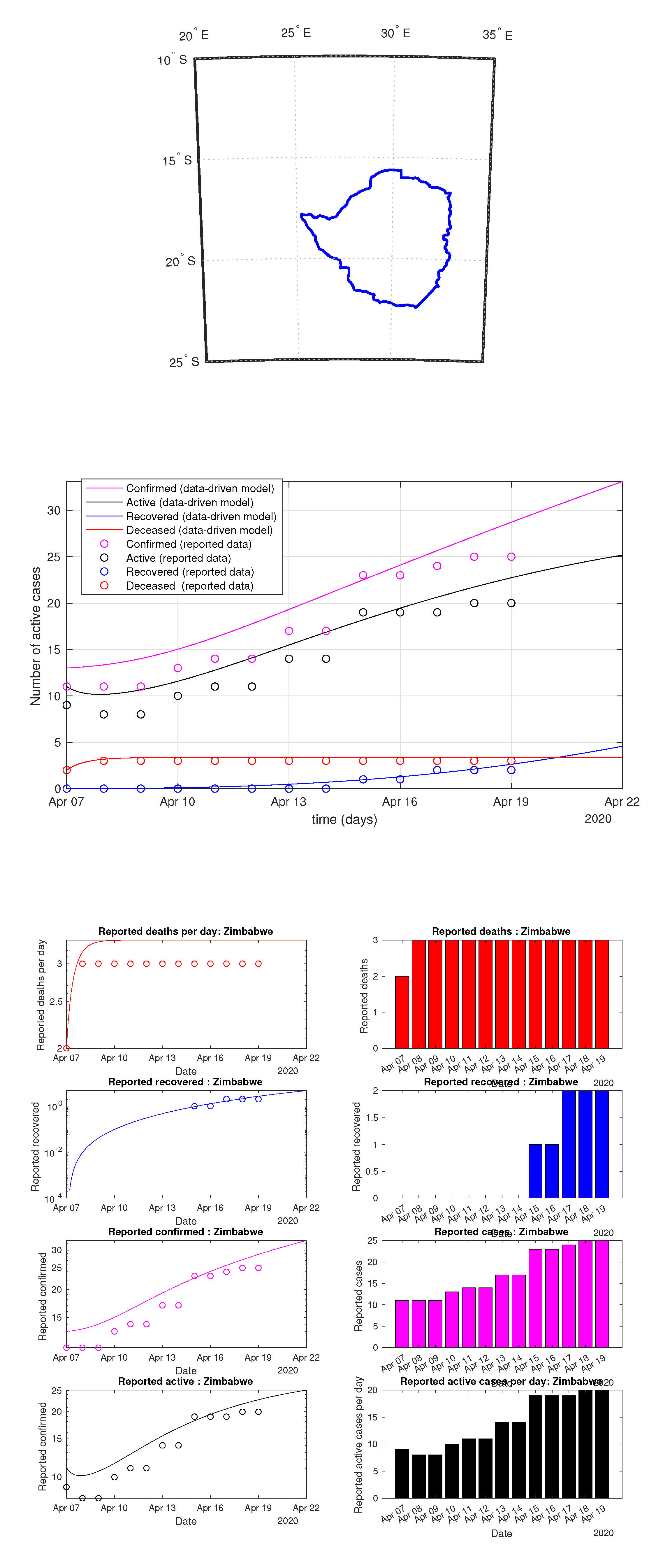
Table 1.
Key features of the data-driven MFTG model.
| Feature | SIR | SEIR | SEIRD | SEIR-Spatial | SEIR -Age Structured | MFTG |
|---|---|---|---|---|---|---|
| locality | no | no | no | no | no | yes |
| city | no | no | no | no | no | yes |
| sector per city | no | no | no | no | no | yes |
| position | no | no | no | yes | no | yes |
| infection status | 3 states | 4 | 5 | 4 | 4 | 17 |
| age | no | no | no | no | yes | yes |
| gender | no | no | no | no | no | yes |
| height | no | no | no | no | no | yes |
| health | no | no | no | no | no | yes |
| family size | no | no | no | no | no | yes |
| economic status | no | no | no | no | no | yes |
| testing strategy | no | no | no | no | no | yes |
| decision-making | no | no | no | no | no | yes |
| untested positive | no | no | no | no | no | yes |
| data-driven | no | no | no | no | no | yes |
Table 2.
Heterogenous data sources.
| Data | Sources |
|---|---|
| International connectivity per country | Flightradar24 [34] |
| Age structure per country | [35] |
| COVID-19 data set | [10,11,12,13,36] |
| Local mobility | Google Community |
| Mobility Reports [37] | |
| Country-specific hospital capacity data | World Bank Group [38] |
| Geographical map | OpenStreet map |
| Economic policy | IMF |
Table 3.
Some notations used the proposed model.
| Symbols | Meaning |
|---|---|
| l | locality |
| country, city, area | |
| temperature field | |
| migration between countries | |
| migration between cities | |
| local mobility between areas of a city | |
| z | age variable |
| initial age distribution | |
| testing capacity per week | |
| testing strategy at l | |
| pre-existing health condition, | |
| gender, height, family size, economic wealth | |
| position of an individual agent | |
| v | velocity of an individual agent |
| s | individual epidemiological states |
| subpopulation size at locality l | |
| u | meeting/activity strategy |
| m | mean-field |
| f | Drift |
| interaction kernel | |
| physical distancing of 2 m | |
| e | economic wealth |
Table 4.
List 1 of figures and illustrations.
| Illustration | Meaning |
|---|---|
| Figure 1 | Flow diagram |
| Figure 3 | first wave of spread |
| Figure 4 | death rate distribution by age |
| Figure 5 | sample age distribution |
| Figure 6 | evolution of the epidemiological ODE with 17 states |
| Figure 8 | connection with SIR |
| Figure 9 | connection with SEIR |
| Figure 10 | connection with SIRD |
| Figure 11 | connection with SEIRD |
| Figure 2 | pandemic vs. economic |
| consequences of COVID-19 | |
| Figure 12 | spread worldwide |
| Figure 13 | propagation of the virus in |
| 15 most reported active cases | |
| as of 11 April 2020 | |
| Figure 14 | G7 countries |
| Figure 15 | New York and Los Angeles |
| testing results: data vs. model | |
| Figure 18 | Brazil: Sequential data-driven model |
| Figure 19 | USA: Sequential data-driven model |
Table 5.
List 2 of figures and illustrations. data of active, recovered, deceased (in circle or bar) vs. model of active, recovered, deceased over time. Tracking the number of active cases. Predictive analytics for the next couple days.
Table 5.
List 2 of figures and illustrations. data of active, recovered, deceased (in circle or bar) vs. model of active, recovered, deceased over time. Tracking the number of active cases. Predictive analytics for the next couple days.
| Illustration | Meaning |
|---|---|
| Figure 20 | Argentina: data vs. model |
| Figure 21 | Bolivia: data vs. model |
| Figure 22 | Brazil: data vs. model |
| Figure 23 | Chile: data vs. model |
| Figure 24 | Colombia: data vs. model |
| Figure 25 | Ecuador: data vs. model |
| Figure 26 | Paraguay: data vs. model |
| Figure 27 | Peru: data vs. model |
| Figure 28 | Uruguay: data vs. model |
| Figure 29 | Venezuela: data vs. model |
| Figure 30 | Cuba: data vs. model |
| Figure 31 | Guatemala: data vs. model |
| Figure 32 | Haiti: data vs. model |
| Figure 33 | Mexico: data vs. model |
| Figure 34 | Bangladesh: data vs. model |
| Figure 35 | India: data vs. model |
| Figure 36 | Indonesia: data vs. model |
| Figure 37 | Korea: data vs. model |
| Figure 38 | Malaysia: data vs. model |
| Figure 39 | Pakistan: data vs. model |
| Figure 40 | UAE: data vs. model |
| Figure 41 | Germany: data vs. model |
| Figure 42 | Italy: data vs. model |
| Figure 43 | Russia: data vs. model |
| Figure 44 | Spain: data vs. model |
| Figure 16 | Non-Gaussianity and non-exponential |
| Figure 17 | Not a single exponential |
Table 6.
List 3 of figures and illustrations. data of active, recovered, deceased (in circle or bar) vs. model of active, recovered, deceased over time. Tracking the number of active cases. Predictive analytics for the next couple days.
Table 6.
List 3 of figures and illustrations. data of active, recovered, deceased (in circle or bar) vs. model of active, recovered, deceased over time. Tracking the number of active cases. Predictive analytics for the next couple days.
| Illustration | Meaning |
|---|---|
| Figure 45 | Covid-19 samples in selected countries in Africa |
| Figure 46 | Selected COMESA countries |
| Figure 47 | Selected ECOWAS countries |
| Figure 48 | Selected SADC countries |
| Figure 49 | Tunisia: Sequential data-driven model |
| Figure 50 | Algeria: data vs. model |
| Figure 51 | Angola: data vs. model |
| Figure 52 | Botswana: data vs. model |
| Figure 53 | Benin: data vs. model |
| Figure 54 | Burkina Faso: data vs. model |
| Figure 55 | Burundi: data vs. model |
| Figure 56 | Cameroon: data vs. model |
| Figure 57 | Chad: data vs. model |
| Figure 58 | Djibouti: data vs. model |
| Figure 59 | Egypt: data vs. model |
| Figure 60 | Eritrea: data vs. model |
| Figure 61 | Eswatini: data vs. model |
Table 7.
List 4 of figures and illustrations. data of active, recovered, deceased (in circle or bar) vs. model of active, recovered, deceased over time. Tracking the number of active cases. Predictive analytics for the next couple days.
Table 7.
List 4 of figures and illustrations. data of active, recovered, deceased (in circle or bar) vs. model of active, recovered, deceased over time. Tracking the number of active cases. Predictive analytics for the next couple days.
| Illustration | Meaning |
|---|---|
| Figure 62 | Ethiopi: data vs. model |
| Figure 63 | Gabon: data vs. model |
| Figure 64 | Ghana: data vs. model |
| Figure 65 | Guinea: data vs. model |
| Figure 66 | Guinea Bissau: data vs. model |
| Figure 67 | Kenya: data vs. model |
| Figure 68 | Liberia: data vs. model |
| Figure 69 | Libya: data vs. model |
| Figure 70 | Madagascar: data vs. model |
| Figure 71 | Malawi: data vs. model |
| Figure 72 | Mali: data vs. model |
| Figure 73 | Mauritania: data vs. model |
| Figure 74 | Mauritius: data vs. model |
| Figure 75 | Morocco: data vs. model |
| Figure 76 | Mozambique: data vs. model |
| Figure 77 | Namibia: data vs. model |
| Figure 78 | Niger: data vs. model |
| Figure 79 | Nigeria: data vs. model |
| Figure 80 | Rwanda: data vs. model |
| Figure 81 | Senegal: data vs. model |
| Figure 82 | Seychelles: data vs. model |
| Figure 83 | Somalia: data vs. model |
| Figure 84 | South Africa: data vs. model |
| Figure 85 | Sudan: data vs. model |
| Figure 86 | Togo: data vs. model |
| Figure 87 | Tunisia: data vs. model |
| Figure 88 | Uganda: data vs. model |
| Figure 89 | Zambia: data vs. model |
| Figure 90 | Zimbabwe: data vs. model |
Publisher’s Note: MDPI stays neutral with regard to jurisdictional claims in published maps and institutional affiliations. |
© 2020 by the author. Licensee MDPI, Basel, Switzerland. This article is an open access article distributed under the terms and conditions of the Creative Commons Attribution (CC BY) license (http://creativecommons.org/licenses/by/4.0/).
Share and Cite
MDPI and ACS Style
Tembine, H. COVID-19: Data-Driven Mean-Field-Type Game Perspective. Games 2020, 11, 51. https://doi.org/10.3390/g11040051
AMA Style
Tembine H. COVID-19: Data-Driven Mean-Field-Type Game Perspective. Games. 2020; 11(4):51. https://doi.org/10.3390/g11040051
Chicago/Turabian StyleTembine, Hamidou. 2020. "COVID-19: Data-Driven Mean-Field-Type Game Perspective" Games 11, no. 4: 51. https://doi.org/10.3390/g11040051
Note that from the first issue of 2016, this journal uses article numbers instead of page numbers. See further details here.