Hierarchical Structures and Leadership Design in Mean-Field-Type Games with Polynomial Cost

Abstract

This article presents a class of hierarchical mean-field-type games with multiple layers and non-quadratic polynomial costs. The decision-makers act in sequential order with informational differences. We first examine the single-layer case where each decision-maker does not have the information about the other control strategies. We derive the Nash mean-field-type equilibrium and cost in a linear state-and-mean-field feedback form by using a partial integro-differential system. Then, we examine the Stackelberg two-layer problem with multiple leaders and multiple followers. Numerical illustrations show that, in the symmetric case, having only one leader is not necessarily optimal for the total sum cost. Having too many leaders may also be suboptimal for the total sum cost. The methodology is extended to multi-level hierarchical systems. It is shown that the order of the play plays a key role in the total performance of the system. We also identify a specific range of parameters for which the Nash equilibrium coincides with the hierarchical solution independently of the number of layers and the order of play. In the heterogeneous case, it is shown that the total cost is significantly affected by the design of the hierarchical structure of the problem.

1. Introduction

The idea of hierarchy dates back at least to 1934, when Stackelberg [1] introduced a game that models markets where some firms have a stronger influence on others. Stackelberg games consist of two players, a leader and a follower. The leader who moves first decides an optimal strategy after anticipating the best response of the follower. Then, the follower eventually chooses the anticipated best response to optimize their cost or payoff. Therefore, this game is a game with two-level hierarchy. A dynamic Linear-Quadratic (LQ) Stackelberg differential game was studied by Samaan and Cruz [2]. A stochastic LQ Stackelberg differential game was investigated by Bagchi and Başar [3]. Bensoussan et al. [4] derived a maximum principle for the leader’s Stackelberg solution under the adapted closed-loop memoryless information structure.

Having two or more players, the Stackelberg game is called a hierarchical game, and it becomes more interesting and involved due to its multi-layer structure, including various forms of information. The players act in sequential order, such that each one of them is a leader for the previous and a follower of the next player in the hierarchy. For hierarchical mean-field-free differential games, see, for example, [5,6,7,8,9].

Only a few papers have considered hierarchical structures in mean-field-related games. Open-loop Stackelberg solutions are addressed in a linear-quadratic setting in [10,11]; and in the context of large populations, mean-field Stackelberg games are investigated in [12,13,14,15,16]. Besides, the leader-follower configuration has been used in several problems and fields to illustrate and model a variety of hierarchical behaviors. For instance, in [17], a leader-follower stochastic differential game with asymmetric information is studied, motivated by applications in finance, economics, and management engineering. In [18], a large-population leader-follower stochastic multi-agent system is analyzed with coupled cost functions and by using a mean-field Linear-Quadratic-Gaussian (LQG) approach. Regarding control applications, [19] presents a tracking control design in a distributed manner in a multi-agent system configured in a leader-follower fashion, and it is shown that the setup can be used to model the power sharing problem in microgrids. In [20], a security problem in networked control systems is studied by means of a Stackelberg approach, and in [21] a hierarchical control structure or sequential predictive control is designed for a large-scale water system. In [22], leadership is studied in the context of public goods games by means of the reward and punishment effects. The works mentioned above do not consider a hierarchical mean-field-type game setting where the payoff functionals are non-linear with respect to the probability measure of the state.

mean-field-type control was first introduced by Anderson and Djehiche [23], as well as Buckdahn, Djehiche, and Li [24]. The authors solved a one-player mean-field-type game in which the state dynamics and the payoff function depend on the first moment of the state (the mean-field coupling). The stochastic mean-field-type control problem is generalized to the stochastic mean-field-type game with several players—see, for example, [25,26,27,28,29,30,31].

The hierarchical mean-field-type game theory studies a class of hierarchical games in which the payoffs and/or state dynamics depend not only on the state-action pairs, but also the distribution of them [30]. This class of games offers several features:

• A single decision-maker can have a strong impact on the mean-field terms;
• The expected payoffs are not necessarily linear with respect to the state distribution;
• The number of decision-makers is not necessarily infinite.

Games with non-linear distribution-dependent quantity-of-interest are very attractive in terms of applications, since the non-linear dependence of the payoff functions in terms of state distribution allow us to capture risk measures, which are functionals of variance, inverse quantile, and/or higher moments. In portfolio optimization, for instance, payoff functions may include the third and the fourth moments, known as the kurtosis and skewness (e.g., [32,33]). Generally, equilibrium solutions to mean-field-type games are presented as either open-loop or closed-loop solutions. The open-loop solutions are controls that do not explicitly depend on the state process at time t, that is, they are rather adapted processes that depend only on time and the initial data. The stochastic maximum principle can be used as a methodology for finding such optimal control strategies. Closed-loop solutions (i.e., feedback solutions) are deterministic functions that depend on the state of the process at time t, as well as its marginal distribution. The dual adjoint functions which are obtained from the Hamilton-Jacobi-Bellman (HJB) equations can be used for finding feedback optimal controls. We will use this approach throughout this paper. For linear quadratic stochastic differential games, Sun and Yong [34] established that the existence of open-loop optimal control strategies is equivalent to the solvability of the corresponding optimality system, which is a forward-backward Stochastic Differential Equation (SDE), and the existence of closed-loop optimal strategies is equivalent to the existence of a regular solution to the corresponding Riccati equation.

Our contribution can be summarized as follows. This work examines a class of hierarchical mean-field-type games with multiple layers, leaders, and followers. Based on infinite-dimensional partial integro-differential equations (PIDEs) on the space of measures, we provide semi-explicit solutions in closed-loop form of a class of master systems with hierarchical structure and non-quadratic cost, which are not covered in the earlier works. Recall that the non-quadratic costs allow for analysis other classes of higher risk terms, such as kurtosis [32,33]. The novelty of this paper mainly lies in the analysis of the effect of hierarchy and leadership on the solutions.

The rest of this article is structured as follows. We present the model setup in Section 2. Section 3 investigates the Nash equilibrium (no leader). Section 4 presents the Stackelberg solution. The multi-layer case is presented in Section 5. Numerical examples are presented in Section 6. Finally, concluding remarks are drawn in Section 7.

2. The Setup

There are $I\ge 2$ decision-makers interacting within the time horizon $[t_0,t_1],t_0<t_1.$ The set of decision-makers is denoted by $\mathcal{I}=\{1,2,\dots ,I\}.$ Decision-maker $i\in \mathcal{I}$ has a control action $u_i\in U_i=\mathbb{R}.$ The state x is driven by a Drift-Jump-Diffusion process of mean-field-type, given by

$$dx=bdt+\sigma dB+{\int }_{\mathsf{\Theta }}\mu (.,\theta )\tilde{N}(dt,d\theta ),x\left(t_0\right)\sim m(t_0,.),$$

where

• $\mathrm{Drift}:b:[t_0,t_1]\times \mathbb{R}\times {\prod }_{j=1}^I{U}_j\times \mathcal{P}\left(\mathbb{R}\right)\to \mathbb{R},$
• $\mathrm{Diffusion} \mathrm{coefficient}:\sigma :[t_0,t_1]\times \mathbb{R}\times {\prod }_{j=1}^I{U}_j\times \mathcal{P}\left(\mathbb{R}\right)\to \mathbb{R},$
• $\mathrm{Brownian} \mathrm{motion}B,$
• $\mathrm{Set} \mathrm{of} \mathrm{jump} \mathrm{size}:\mathsf{\Theta }={\mathbb{R}}_{+}\backslash \left\{0\right\},$
• $\mathrm{Jump}:N(dt,d\theta ),$
• $\mathrm{Compensated} \mathrm{jump}:\tilde{N}(dt,d\theta )=N(dt,d\theta )-\nu \left(d\theta \right)dt,$
• $\mathrm{Jump} \mathrm{rate}:\mu :[t_0,t_1]\times \mathbb{R}\times {\prod }_{j=1}^I{U}_j\times \mathcal{P}\left(\mathbb{R}\right)\times \mathsf{\Theta }\to \mathbb{R},$

where $\mathcal{P}\left(\mathbb{R}\right)$ denotes the set of probability measures on $\mathbb{R}.$ We assume that $x\left(t_0\right),B$ and N are mutually independent. The performance functional of decision-maker i is

$$L_i(u,m_0)=h_i(x\left(t_1\right),m\left(t_1\right))+{\int }_{t_0}^{t_1}{l}_i(t,x,u,m)dt,$$

where $m(t,dy)={\mathbb{P}}_{x\left(t\right)}\left(dy\right)$ is the probability measure of the state $x\left(t\right)$ at time $t,$ and

$$\begin{array}{c}{l}_i:[t_0,t_1]\times \mathbb{R}\times \prod _{j=1}^I{U}_j\times \mathcal{P}\left(\mathbb{R}\right)\to \mathbb{R},\hfill \\ h_i:\mathbb{R}\times \mathcal{P}\left(\mathbb{R}\right)\to \mathbb{R}.\hfill \end{array}$$

In addition, each decision-maker is assumed to have a computational capability, such as being able to compute an aggregative term of m from the model. Let ${\mathcal{U}}_i$ be the set of control strategies of decision-maker i that are progressively measurable with respect to the filtration generated by the unions of events in $\{B,N\}.$

2.1. Games with Polynomial Cost

We investigate the mean-field-type game with the following data:

$$\begin{array}{cc}\hfill t_0& =0,t_1=T>0,\hfill \\ \hfill l_i(t,x,u,m)& =q_i\frac{{(x-\overline{x})}^{2k_i}}{2k_i}+r_i\frac{{(u_i-{\overline{u}}_i)}^{2k_i}}{2k_i}+c_i{(x-\overline{x})}^{2k_i-1}(u_i-{\overline{u}}_i)\hfill \\ \hfill & +\sum _{j\in \mathcal{I}\backslash \left\{i\right\}}{ϵ}_{ij}{(x-\overline{x})}^{2(k_i-1)}(u_i-{\overline{u}}_i)(u_j-{\overline{u}}_j)\hfill \end{array}$$

(1a)

$$\begin{array}{cc}\hfill & +{\overline{q}}_i\frac{{\overline{x}}^{2{\overline{k}}_i}}{2{\overline{k}}_i}+{\overline{r}}_i\frac{{\overline{u}}_i^{2{\overline{k}}_i}}{2{\overline{k}}_i}+{\overline{c}}_i{\overline{x}}^{2{\overline{k}}_i-1}{\overline{u}}_i+\sum _{j\ne i}{\overline{ϵ}}_{ij}{\overline{x}}^{2({\overline{k}}_i-1)}{\overline{u}}_i{\overline{u}}_j,\hfill \end{array}$$

(1b)

$$\begin{array}{cc}\hfill h_i(x,m)& =q_{iT}\frac{{(x_T-{\overline{x}}_T)}^{2k_i}}{2k_i}+{\overline{q}}_{iT}\frac{{\overline{x}}_T^{2{\overline{k}}_i}}{2{\overline{k}}_i},\hfill \end{array}$$

(1c)

$$\begin{array}{cc}\hfill b(t,x,u,m)& =b_1(x-\overline{x})+{\overline{b}}_1\overline{x}+\sum _{j\in \mathcal{I}}\left[b_{2j}(u_j-{\overline{u}}_j)+{\overline{b}}_{2j}{\overline{u}}_j\right],\hfill \end{array}$$

(1d)

$$\begin{array}{cc}\hfill \sigma (t,x,u,m)& =(x-\overline{x})\tilde{\sigma },\hfill \end{array}$$

(1e)

$$\begin{array}{cc}\hfill \mu (t,x,u,m,\theta )& =(x-\overline{x})\tilde{\mu }(.,\theta ),\hfill \end{array}$$

(1f)

$$\begin{array}{cc}\hfill \overline{x}\left(t\right)& =\int ym(t,dy),\hfill \end{array}$$

(1g)

$$\begin{array}{cc}\hfill {\overline{u}}_i\left(t\right)& =\int u_i(t,y,m)m(t,dy),i\in \mathcal{I},\hfill \end{array}$$

(1h)

where $k_i\ge 1,{\overline{k}}_i\ge 1,$ are natural numbers, and the coefficients are time-dependent. The coefficient functions $q_i,r_i,$${\overline{q}}_i$ and ${\overline{r}}_i$ are nonnegative functions, and

$$\begin{array}{c}\hfill {\int }_{t_0}^{t_1}\left[{\tilde{\sigma }}^2\left(t\right)+{\int }_{\mathsf{\Theta }}\left({(1+\tilde{\mu }(t,\theta ))}^{2k_i}-1-2k_i\tilde{\mu }(t,\theta )\right)\nu \left(d\theta \right)\right]dt<+\infty .\end{array}$$

2.2. Hierarchical Leader Design and Algorithmic Approach

The hierarchical leadership design consists of finding the optimal number of hierarchical layers h and the non-empty subsets of players ${\mathcal{I}}_1,\dots ,{\mathcal{I}}_h$, partitioning the set of all players as

$$\mathcal{I}=\bigcup _{k=1}^h{\mathcal{I}}_k,\mathrm{and}\mathrm{if}k\ne k^{\prime },{\mathcal{I}}_k\cap {\mathcal{I}}_{k^{\prime }}=\varnothing .$$

The performance functional for the hierarchical design is the sum cost at the chosen hierarchical solution, that is,

$$\underset{h}{inf}\underset{({\mathcal{I}}_1,\dots ,{\mathcal{I}}_h):{\cup }_{k=1}^h{\mathcal{I}}_k=\mathcal{I}}{inf}S(h,{\mathcal{I}}_1,\dots ,{\mathcal{I}}_h).$$

Here, we take into consideration three main game scenarios, described as follows. First, the game has a unique layer, that is, a situation in which all the players select their strategies simultaneously. Second, the game is played in two layers (bi-level hierarchy). The players are grouped into two sets ($h=2$): leaders, which are those who decide first, as well as simultaneously; and followers, which are those who react against the decision of the leaders. Third, the game is structured to take into account as many layers as the number of players (fully hierarchical configuration with $h=I$), that is, players select strategically in sequence one-by-one in I layers. For all configurations, let $L_i^{*}$ denote the optimal cost of the player $i\in \mathcal{I}$ in the hierarchical mean-field-type game problem, and $S(h,{\mathcal{I}}_1,\dots ,{\mathcal{I}}_h)={\sum }_{i\in \mathcal{I}}{L}_i^{*}$ denotes the total (social) cost at the hierarchical solution. The hierarchical leadership design consists in determining the optimal leaders, followers, and/or number of layers, such that the total cost is minimized.

Notice that, for both the bi-level and fully hierarchical cases, there are multiple combinations for the players. In the bi-level scenario, the set of all possible sets of leaders is given by the power set $2^{\mathcal{I}},$ and any set of leaders is denoted by ${\mathcal{I}}_L\subseteq 2^{\mathcal{I}}$ with the corresponding set of followers, ${\mathcal{I}}_F=\mathcal{I}\backslash {\mathcal{I}}_L$. Regarding the fully hierarchical game, there are as many possibilities in the strategic ordering as permutations of the set of players $\mathcal{I}$. All possible permutations of the players are considered.

For the bi-level case, the optimal set for leaders and followers is

$$\begin{array}{cc}\hfill {\mathcal{I}}_L^{*}& \in arg\underset{2^{\mathcal{I}}}{min}S(2,{\mathcal{I}}_1,{\mathcal{I}}_2),\hfill \\ \hfill {\mathcal{I}}_F^{*}& =\mathcal{I}\backslash {\mathcal{I}}_L^{*}.\hfill \end{array}$$

On the other hand, for the fully hierarchical case, we have that the optimal permutation is

$$\begin{array}{cc}\hfill ({\mathcal{I}}_1^{*},\dots ,{\mathcal{I}}_I^{*})& \in arg\underset{{\mathcal{I}}_1,\dots ,{\mathcal{I}}_I}{min}S(I,{\mathcal{I}}_1,\dots ,{\mathcal{I}}_I).\hfill \end{array}$$

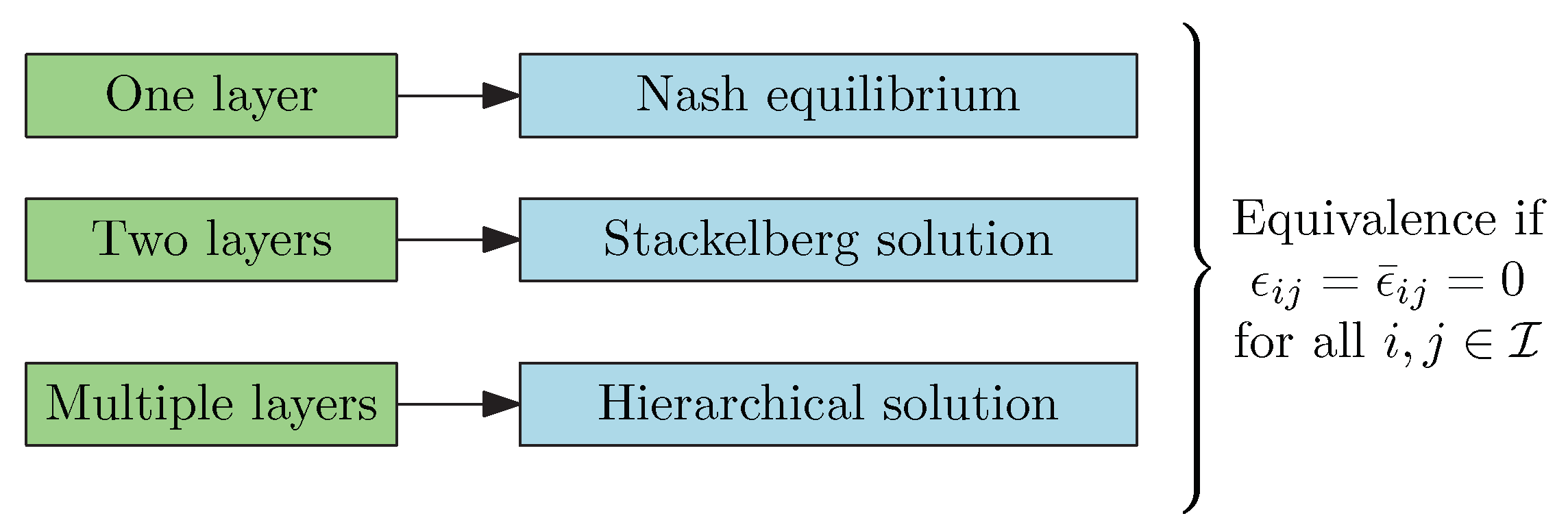
In this paper, we study the three aforementioned scenarios involving one, two, and I layers, as presented in Figure 1. We also present under which conditions all the three configurations have the same solution, that is, when the Nash solution coincides with the hierarchical solutions at different layers. Furthermore, we present numerical examples considering different levels of hierarchy. The problem addressed in this paper can be interpreted as a mechanism design that, instead of determining the appropriate cost functionals or utility functions to induce a desired output, we design the best hierarchical structure in order to reduce the overall social cost.

Remark 1

(Feasibility and Existence). The set of possible combinations for the layers/levels and players per level is non-empty and finite. Then, the optimal hierarchical leader design is feasible, and there exists an optimal solution (combination) such that the social cost is minimized.

Since the feasible set of possible combinations for the hierarchical configurations is non-empty and finite, then it is possible to find the best hierarchical structure by means of Algorithm 1. The main results evoked in the Algorithm 1, given by Propositions 1–3, are presented throughout the paper.

Algorithm 1: Finding the best hierarchical structure

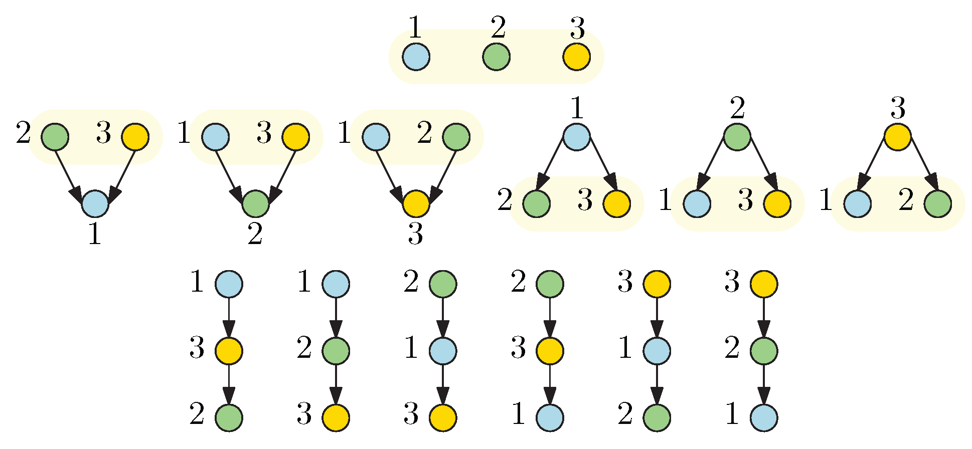
According to the procedure in Algorithm 1, one of the main concerns in the leadership design problem is related to the dimensionality of the feasible set for the hierarchical structures (NP-hard problem). The total number of combinations is, given by the total number of ordered partitions from a set, where such total combinations are computed by means of the ordered Bell number $B:\mathbb{N}\to \mathbb{N}$—that is, for I players we have:

$$B\left(I\right)=\sum _{k=0}^I\sum _{j=0}^k{(-1)}^{k-j}\left(\begin{array}{c}k\\ j\end{array}\right)j^n.$$

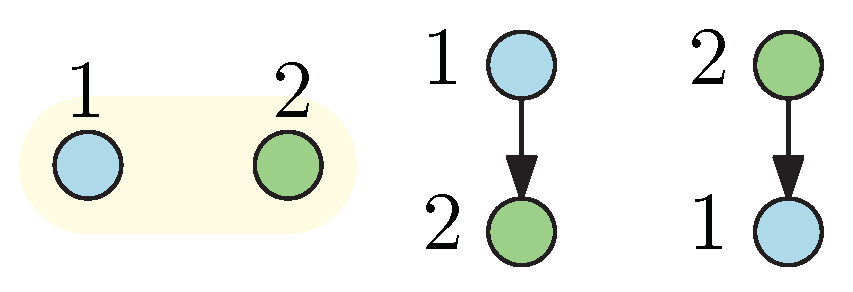
For instance, if $I=2$, then there are $B\left(2\right)=3$ possible leadership configurations, as shown in Figure 2; i $I=3$, and then there are $B\left(3\right)=13$ possible leadership structures presented in Figure 3, and $B\left(4\right)=75$, $B\left(5\right)=541$, and $B\left(6\right)=4683$. Figure 4 illustrates the rapid increment of the number of combinations as the decision-makers increase. Notice that it is not possible to have more levels than players in the hierarchical game ($h\le I$). The following sections are devoted to the presentation of semi-explicit solutions for hierarchical mean-field-type games with different levels from one (Nash scenario) up to the number of players I (fully hierarchical scenario).

3. Nash Mean-Field-Type Equilibrium

The risk-neutral mean-field-type game is, given by

$${(\mathcal{I},U_i,{\mathcal{U}}_i,\mathbb{E}\left[L_i\right])}_{i\in \mathcal{I}}.$$

A risk-neutral Nash mean-field-type Equilibrium is a solution of the following fixed-point problem:

$$\begin{array}{cc}\hfill & i\in \mathcal{I},\hfill \\ \hfill & \mathbb{E}\left[L_i\left(u^{*}\right)\right]=\underset{u_i\in {\mathcal{U}}_i}{inf}\mathbb{E}\left[L_i(u_1^{*},\dots ,u_{i-1}^{*},u_i,u_{i+1}^{*},\dots ,u_I^{*})\right].\hfill \end{array}$$

Let ${\widehat{V}}_i(t,m)$ be the optimal cost-to-go from m at time $t\in (t_0,t_1)$ given the strategies of the others, that is,

$$\begin{array}{cc}\hfill {\widehat{V}}_i(t,m)& =\underset{u_i}{inf}\mathbb{E}[h_i(x\left(t_1\right),m\left(t_1\right))+{\int }_t^{t_1}{l}_i(t,x,u,m)d{t}^{\prime }|m\left(t\right)=m].\hfill \end{array}$$

We say that ${\widehat{V}}_{i,m}(t,x,m):={\widehat{V}}_{i,m}(t,m)\left(x\right)$ is a Gâteaux derivative of ${\widehat{V}}_i(t,m)$, with respect to the measure m, if

$$\underset{\tau \to 0}{lim}\frac{d}{d\tau }{\widehat{V}}_i(t,m+\tau \tilde{m})=\int {\widehat{V}}_{i,m}(t,m)\left(x\right)\tilde{m}\left(dx\right).$$

(2)

If $\int \tilde{m}\left(dx\right)=0$, then adding a constant to ${\widehat{V}}_{i,m}(t,x,m)$ does not change the value of the integral in (2). For any scalar $\lambda$ and $m\in \mathcal{P}\left(\mathbb{R}\right)$ one has, $\lambda =\lambda \int m\left(dx\right).$ Thus, $\lambda$ is also a Gâteaux-derivative of the constant function $\lambda .$ However, in our problem, the term ${\widehat{V}}_{i,xm}$, which is the gradient of $x\mapsto {\widehat{V}}_{i,m}(t,x,m)$, will be used in the Hamiltonian, and ${\widehat{V}}_{i,xm}$ does not have the constant ambiguity. Let us denote the jump operator J as

$$J\left[{\varphi }_i\right]:={\int }_{\mathsf{\Theta }}[{\varphi }_{i,m}(t^{-},x+\mu )-{\varphi }_{i,m}-\mu {\varphi }_{i,xm}]\nu \left(d\theta \right).$$

Let us introduce the integrand Hamiltonian as

$$\begin{array}{cc}\hfill H_i(t,x,m,{\widehat{V}}_m,& {\widehat{V}}_{xm},{\widehat{V}}_{xxm})\hfill \\ \hfill & =\underset{u_i\in U_i}{inf}\left\{l_i+b{\widehat{V}}_{i,xm}+\frac{{\sigma }^2}{2}{\widehat{V}}_{i,xxm}+{\int }_{\mathsf{\Theta }}[{\widehat{V}}_{i,m}(t^{-},x+\mu )-{\widehat{V}}_{i,m}-\mu {\widehat{V}}_{i,xm}]\nu \left(d\theta \right)\right\}.\hfill \end{array}$$

A sufficiency condition for a risk-neutral Nash equilibrium system is, given by the following PIDE system:

$$\begin{array}{cc}\hfill 0& ={\widehat{V}}_{i,t}(t,m)+\int H_i(t,x,m,{\widehat{V}}_m,{\widehat{V}}_{xm},{\widehat{V}}_{xxm})m\left(dx\right),\hfill \end{array}$$

(3a)

$$\begin{array}{cc}\hfill {\widehat{V}}_i(t_1,m)& =\int m\left(dy\right)h_i(y,m),i\in \mathcal{I}.\hfill \end{array}$$

(3b)

We refer the reader to [35] for a derivation of this equilibrium system. The system (3) is an infinite-dimensional PIDE system in m and it provides the Nash equilibrium values of the mean-field-type game. Notice that from (3), the equilibrium strategies have the best response to the integrand Hamiltonian and can be expressed as functions of $t,x,m,{\widehat{V}}_{i,m},{\widehat{V}}_{i,xm},{\widehat{V}}_{i,xxm}.$

Next, we semi-explicitly provide the Nash mean-field-type equilibrium in linear state-and-mean -field feedback strategies. To do so, we use (3).

Proposition 1.

A risk-neutral Nash mean-field-type equilibrium is given in a semi-explicit way, as follows:

$$\begin{array}{cc}\hfill u_i^{ne}& =-{\eta }_i\left(x-\int ym(dy)\right)-{\overline{\eta }}_i\int ym\left(dy\right),\hfill \end{array}$$

(4a)

$$\begin{array}{cc}\hfill 0& =-r_i{\eta }_i^{2k_i-1}-\sum _{j\ne i}{ϵ}_{ij}{\eta }_j+b_{2i}{\alpha }_i+c_i,\hfill \end{array}$$

(4b)

$$\begin{array}{cc}\hfill 0& =-{\overline{r}}_i{\overline{\eta }}_i^{2{\overline{k}}_i-1}-\sum _{j\ne i}{\overline{ϵ}}_{ij}{\overline{\eta }}_j+{\overline{b}}_{2i}{\overline{\alpha }}_i+{\overline{c}}_i,\hfill \end{array}$$

(4c)

$$\begin{array}{cc}\hfill {\widehat{V}}_i(t,m)& ={\alpha }_i{\int }_x\frac{{(x-\int ym\left(dy\right))}^{2k_i}}{2k_i}m\left(dx\right)+{\overline{\alpha }}_i\frac{{(\int ym\left(dy\right))}^{2{\overline{k}}_i}}{2{\overline{k}}_i},\hfill \\ \hfill 0& ={\dot{\alpha }}_i+q_i+r_i{\eta }_i^{2k_i}-2k_i{c}_i{\eta }_i+2k_i\sum _{j\ne i}{ϵ}_{ij}{\eta }_i{\eta }_j+2k_i{\alpha }_i[b_1-\sum _{j\in \mathcal{I}}{b}_{2j}{\eta }_j]+2k_i(2k_i-1){\alpha }_i\frac{1}{2}{\tilde{\sigma }}^2\hfill \end{array}$$

(4d)

$$\begin{array}{cc}\hfill & +{\alpha }_i{\int }_{\mathsf{\Theta }}\left[{(1+\tilde{\mu })}^{2k_i}-1-2k_i\tilde{\mu }\right]\nu \left(d\theta \right),\hfill \end{array}$$

(4e)

$$\begin{array}{cc}\hfill {\alpha }_i\left(T\right)& =q_{iT},\hfill \end{array}$$

(4f)

$$\begin{array}{cc}\hfill 0& ={\dot{\overline{\alpha }}}_i+{\overline{q}}_i+{\overline{r}}_i{\overline{\eta }}_i^{2{\overline{k}}_i}-2{\overline{k}}_i{\overline{c}}_i{\overline{\eta }}_i+2{\overline{k}}_i\sum _{j\ne i}{\overline{ϵ}}_{ij}{\overline{\eta }}_i{\overline{\eta }}_j+2{\overline{k}}_i{\overline{\alpha }}_i\left[{\overline{b}}_1-\sum _j{\overline{b}}_{2j}{\overline{\eta }}_j\right],\hfill \end{array}$$

(4g)

$$\begin{array}{cc}\hfill {\overline{\alpha }}_i\left(T\right)& ={\overline{q}}_{iT},\hfill \end{array}$$

(4h)

for all $i\in \mathcal{I}$ with

$$\begin{array}{cc}\hfill \int ym(t,dy)& =\left[\int ym(0,dy)\right]e^{{\int }_0^t\left[{\overline{b}}_1-{\sum }_j{\overline{b}}_{2j}{\overline{\eta }}_j\right]d{t}^{\prime }},\hfill \end{array}$$

(4i)

whenever the above coefficient system admits a solution which does not escape within $[t_0,t_1]$.

Proof. 

The proof is presented in Appendix A. □

The following Remark discusses the existence and uniqueness of the $\eta$ terms in Proposition 1.

Remark 2.

The uniqueness of the coefficient system (4) in η requires a strong condition, that is,

$$0=-r_i{\eta }_i^{2k_i-1}-\sum _{j\ne i}{ϵ}_{ij}{\eta }_j+b_{2i}{\alpha }_i+c_i.$$

• Let I be an arbitrary integer and $k_i=k=1$, the system in η becomes linear and has a unique solution if, and only if the determinant of the matrix M is non-zero, with $M_{ii}=r_i$ and $M_{ij}={ϵ}_{ij},i\ne j.$ When the determinant is zero, the resulting control strategies become non-admissible and the costs become infinite.
• For $k_i=k=2$, and $I=2$ the system in η becomes a binary cubic polynomial, given by

  $$\begin{array}{cc}\hfill r_1{\eta }_1^3+{ϵ}_{12}{\eta }_2-b_{21}{\alpha }_1-c_1& =0,\hfill \\ \hfill r_2{\eta }_2^3+{ϵ}_{21}{\eta }_1-b_{22}{\alpha }_2-c_2& =0.\hfill \end{array}$$
  For ${ϵ}_{12}=0$, there is a unique solution, given by

  $${\eta }_1={\left(\frac{b_{21}{\alpha }_1+c_1}{r_1}\right)}^{\frac{1}{3}},{\eta }_2={\left(\frac{-{ϵ}_{21}{\eta }_1+b_{22}{\alpha }_2+c_2}{r_2}\right)}^{\frac{1}{3}}.$$
  For ${ϵ}_{12}\ne 0$, we derive from the first equation that

  $${\eta }_2=\frac{-r_1{\eta }_1^3+b_{21}{\alpha }_1+c_1}{{ϵ}_{12}}.$$
  By substituting it to the second equation, we arrive at

  $$r_2{\left(\frac{-r_1{\eta }_1^3+b_{21}{\alpha }_1+c_1}{{ϵ}_{12}}\right)}^3+{ϵ}_{21}{\eta }_1-b_{21}{\alpha }_1-c_1=0.$$
  The latter equation is a polynomial of odd degree “9”. It has a unique real root in ${\eta }_1$ if its derivative has a constant sign. Its derivative is

  $${ϵ}_{21}-9\frac{r_1{r}_2}{{ϵ}_{12}}{\eta }_1^2{\left(\frac{-r_1{\eta }_1^3+b_{21}{\alpha }_1+c_1}{{ϵ}_{12}}\right)}^2.$$
  It has a constant sign if ${ϵ}_{21}$ and $\frac{r_1{r}_2}{{ϵ}_{12}}$ have opposite signs. If $r_1$ and $r_2$ are positive, then the condition is reduced to

  $${ϵ}_{21}{ϵ}_{12}\le 0.$$
• $I=2$ and arbitrary $k_i\ge 1$. Thus, a sufficiency condition is that ${ϵ}_{ji}$ and $(2k_i-1)(2k_j-1)\frac{r_i{r}_j}{{ϵ}_{ij}}$ have opposite signs. In particular if $k_i\ge 1,k_j\ge 1,r_i>0,r_j>0$, then the condition reduces to

  $${ϵ}_{ij}{ϵ}_{ji}\le 0.$$
• The same reasoning applies to the system in $\overline{\eta }$, and has a unique real solution if

  $${\overline{ϵ}}_{ij}{\overline{ϵ}}_{ji}\le 0.$$
• For $I\ge 3$ decision-makers and arbitrary $k_i\ge 1$, the system can be rewritten as a fixed-point equation which fulfils a contraction mapping condition if the norms of r and ϵ are sufficiently small. In this case, there is a unique solution.

In the next section, we investigate the bi-level case with multiple leaders and multiple followers.

4. Multiple Leaders and Multiple Followers

We consider the description in (1) in a bi-level hierarchical game with two and more leaders, that is, $|{\mathcal{I}}_L|\ge 2,$ and two and more followers, that is, $|{\mathcal{I}}_F|\ge 2.$ We restrict our attention to the admissible strategies, which are Lipschitz, in the state $x.$ Given the strategies of the leaders ${\left(u_i\right)}_{i\in {\mathcal{I}}_L}\in {\prod }_{i\in {\mathcal{I}}_L}{\mathcal{U}}_i,$ a risk-neutral best-response strategy of follower j is a strategy that solves ${inf}_{{\mathcal{U}}_j}\mathbb{E}{L}_j.$ The set of risk-neutral best responses of j is denoted by ${\mathrm{rnBR}}_j({(u_i)}_{i\in {\mathcal{I}}_L},{(u_{j^{\prime }})}_{j^{\prime }\in {\mathcal{I}}_F\backslash \left\{j\right\}}).$

A mean-field-type risk-neutral Nash equilibrium among the followers given the first movers’ strategies ${\left(u_i\right)}_{i\in {\mathcal{I}}_L}\in {\prod }_{i\in {\mathcal{I}}_L}{\mathcal{U}}_i,$ is a strategy profile $(u_j,j\in {\mathcal{I}}_F)$ of all followers, such that for every decision-maker $j\in {\mathcal{I}}_F,$

$$u_j\in {\mathrm{rnBR}}_j({(u_i)}_{i\in {\mathcal{I}}_L};{(u_{j^{\prime }}^{\mathrm{rn}})}_{j^{\prime }\in {\mathcal{I}}_F\backslash \left\{j\right\}}).$$

The followers solve the following Nash game given the strategy of the leaders ${\left(u_i\right)}_{i\in {\mathcal{I}}_L}$, that is,

$$\begin{array}{cc}\hfill & j\in {\mathcal{I}}_F:\hfill \end{array}$$

$$\begin{array}{cc}\hfill & 0={\widehat{V}}_{j,t}(t,m)+\int H_j^r(x,m,{({\widehat{V}}_{j^{\prime },m},{\widehat{V}}_{j^{\prime },xm},{\widehat{V}}_{j^{\prime },xxm})}_{j^{\prime }\in {\mathcal{I}}_F}|{\left(u_i\right)}_{i\in {\mathcal{I}}_L})m\left(dx\right),\hfill \end{array}$$

(5a)

$$\begin{array}{cc}\hfill & {\widehat{V}}_j(t_1,m)=\int m\left(dy\right)h_j(y,m),\hfill \end{array}$$

(5b)

$$\begin{array}{cc}\hfill & H_j^r=\underset{u_j\in U_j}{inf}\left\{l_j+b{\widehat{V}}_{j,xm}+\frac{{\sigma }^2}{2}{\widehat{V}}_{j,xxm}+J[{\widehat{V}}_{j,m}]|{\left(u_i\right)}_{i\in {\mathcal{I}}_L}\right\}.\hfill \end{array}$$

(5c)

Then, the leaders solve the following PIDE system:

$$\begin{array}{cc}\hfill i& \in {\mathcal{I}}_L:\hfill \end{array}$$

$$\begin{array}{cc}\hfill 0& ={\widehat{V}}_{i,t}(t,m)+\int H_i^r(x,m,{({\widehat{V}}_{i^{\prime },m},{\widehat{V}}_{i^{\prime },xm},{\widehat{V}}_{i,xxm})}_{i^{\prime }\in {\mathcal{I}}_L\cup {\mathcal{I}}_F})m\left(dx\right),\hfill \end{array}$$

(6a)

$$\begin{array}{cc}\hfill {\widehat{V}}_i(t_1,m)& =\int m\left(dy\right)h_i(y,m),\hfill \end{array}$$

(6b)

$$\begin{array}{cc}\hfill H_i^r& =\underset{u_i\in U_i}{inf}\left\{l_i+b{\widehat{V}}_{i,xm}+\frac{{\sigma }^2}{2}{\widehat{V}}_{i,xxm}+J[{\widehat{V}}_{i,m}]|{\{u_j^{*}(.,{\left(u_i\right)}_{i\in {\mathcal{I}}_L})\}}_{j\in {\mathcal{I}}_F}\right\}.\hfill \end{array}$$

(6c)

A minimizer of the integrand Hamiltonian $H_i^r$, denoted by

$$u_i^{ss}=u_i^{ss}(t,x,m,{({\widehat{V}}_{i^{\prime },m},{\widehat{V}}_{i^{\prime },xm},{\widehat{V}}_{i^{\prime },xxm})}_{i^{\prime }\in {\mathcal{I}}_L\cup {\mathcal{I}}_F}),$$

provides a candidate Stackelberg strategy of the leader i. A mean-field-type risk-neutral Stackelberg solution between multiple leaders and multiple followers is a strategy $({(u_i^{ss})}_{i\in {\mathcal{I}}_L},{(u_j^{ss})}_{j\in {\mathcal{I}}_F})$ of all decision-makers, such that

$$\begin{array}{cc}\hfill i& \in {\mathcal{I}}_L,\hfill \\ \hfill u_i^{ss}& \in arg\underset{u_i\in {\mathcal{U}}_i}{min}\left\{\mathbb{E}{L}_i(x,u_i,{(u_{i^{\prime }}^{ss})}_{i\in {\mathcal{I}}_L\backslash \left\{i\right\}},{(u_j^{ss})}_{j\in {\mathcal{I}}_F}):u_j^{ss}\in {\mathrm{rnBR}}_j({(u_i^{ss})}_{i\in {\mathcal{I}}_L};{(u_{j^{\prime }}^{ss})}_{j^{\prime }\in {\mathcal{I}}_F\backslash \left\{j\right\}}\right\},\hfill \end{array}$$

and for every follower,

$$j\in {\mathcal{I}}_F,u_j^{ss}\in {\mathrm{rnBR}}_j({\left(u_i^{ss}\right)}_{i\in {\mathcal{I}}_L};{\left(u_{j^{\prime }}^{ss}\right)}_{j^{\prime }\in {\mathcal{I}}_F\backslash \left\{j\right\}}).$$

The next result presents the Stackelberg mean-field-type solution involving several leaders and followers in a semi-explicit manner.

Proposition 2.

The risk-neutral Stackelberg mean-field-type solution with multiple leaders and multiple followers is given in a semi-explicit way, as follows:

$$\begin{array}{cc}\hfill u_j^{ss}& =-{\eta }_j\left(x-\int ym(dy)\right)-{\overline{\eta }}_j\int ym\left(dy\right),j\in {\mathcal{I}}_F,\hfill \\ \hfill j& \in {\mathcal{I}}_F:\hfill \\ \hfill 0& =-r_j{\eta }_j^{2k_j-1}-\sum _{j^{\prime }\in {\mathcal{I}}_F\backslash \left\{j\right\}}{ϵ}_{j{j}^{\prime }}{\eta }_{j^{\prime }}-\sum _{i\in {\mathcal{I}}_L}{ϵ}_{ji}{\eta }_i+b_{2j}{\alpha }_j+c_j,\hfill \\ \hfill 0& =-{\overline{r}}_j{\overline{\eta }}_j^{2{\overline{k}}_j-1}-\sum _{j^{\prime }\in {\mathcal{I}}_F\backslash \left\{j\right\}}{\overline{ϵ}}_{j{j}^{\prime }}{\overline{\eta }}_{j^{\prime }}-\sum _{i\in {\mathcal{I}}_L}{\overline{ϵ}}_{ji}{\overline{\eta }}_i+{\overline{b}}_{2j}{\overline{\alpha }}_j+{\overline{c}}_j,\hfill \\ \hfill i& \in {\mathcal{I}}_L:\hfill \\ \hfill 0& =-r_i{\eta }_i^{2k_i-1}-\sum _{i^{\prime }\in {\mathcal{I}}_L\backslash \left\{i\right\}}{ϵ}_{i{i}^{\prime }}{\eta }_{i^{\prime }}-\sum _{j\in {\mathcal{I}}_F}{ϵ}_{ij}{\eta }_j+b_{2i}{\alpha }_i+\sum _{j\in {\mathcal{I}}_F}{ϵ}_{ij}{\eta }_i\frac{{ϵ}_{ji}}{(2k_j-1)r_j{\eta }_j^{2k_j-2}}\hfill \\ \hfill & -\sum _{j\in {\mathcal{I}}_F}{b}_{2j}\frac{{ϵ}_{ji}}{(2k_j-1)r_j{\eta }_j^{2k_j-2}}{\alpha }_i+c_i,\hfill \\ \hfill 0& =-{\overline{r}}_i{\overline{\eta }}_i^{2{\overline{k}}_i-1}-\sum _{i^{\prime }\in {\mathcal{I}}_L\backslash \left\{i\right\}}{\overline{ϵ}}_{i{i}^{\prime }}{\overline{\eta }}_{i^{\prime }}-\sum _{j\in {\mathcal{I}}_F}{\overline{ϵ}}_{ij}{\overline{\eta }}_j+{\overline{b}}_{2i}{\overline{\alpha }}_i+\sum _{j\in {\mathcal{I}}_F}{\overline{ϵ}}_{ij}{\overline{\eta }}_i\frac{{\overline{ϵ}}_{ji}}{(2{\overline{k}}_j-1){\overline{r}}_j{\overline{\eta }}_j^{2{\overline{k}}_j-2}}\hfill \\ \hfill & -\sum _{j\in {\mathcal{I}}_F}{\overline{b}}_{2j}\frac{{\overline{ϵ}}_{ji}}{(2{\overline{k}}_j-1){\overline{r}}_j{\overline{\eta }}_j^{2{\overline{k}}_j-2}}{\overline{\alpha }}_i+{\overline{c}}_i,\hfill \end{array}$$

(7a)

and

$$\begin{array}{cc}\hfill {\widehat{V}}_i& (0,m)={\alpha }_i\left(0\right){\int }_x\frac{{(x-\int y{m}_0\left(dy\right))}^{2k_i}}{2k_i}{m}_0\left(dx\right)+{\overline{\alpha }}_i\left(0\right)\frac{{(\int y{m}_0\left(dy\right))}^{2{\overline{k}}_i}}{2{\overline{k}}_i},\hfill \\ \hfill 0& ={\dot{\alpha }}_i+q_i+r_i{\eta }_i^{2k_i}-2k_i{c}_i{\eta }_i+2k_i\sum _{i^{\prime }\in {\mathcal{I}}_L\backslash \left\{i\right\}}{ϵ}_{i{i}^{\prime }}{\eta }_i{\eta }_{i^{\prime }}+2k_i\sum _{j\in {\mathcal{I}}_F}{ϵ}_{ij}{\eta }_i{\eta }_j\hfill \\ \hfill & +2k_i\left[b_1-\sum _{i^{\prime }\in {\mathcal{I}}_L}{b}_{2i^{\prime }}{\eta }_{i^{\prime }}-\sum _{j\in {\mathcal{I}}_F}{b}_{2j}{\eta }_j\right]{\alpha }_i+2k_i(2k_i-1){\alpha }_i\frac{1}{2}{\tilde{\sigma }}^2\hfill \end{array}$$

(7b)

$$\begin{array}{cc}\hfill & +{\alpha }_i{\int }_{\mathsf{\Theta }}[{(1+\tilde{\mu })}^{2k_i}-1-2k_i\tilde{\mu }]\nu \left(d\theta \right),\hfill \end{array}$$

(7c)

$$\begin{array}{cc}\hfill {\alpha }_i& \left(T\right)=q_{iT},\hfill \\ \hfill 0& ={\dot{\overline{\alpha }}}_i+{\overline{q}}_i+{\overline{r}}_i{\overline{\eta }}_i^{2{\overline{k}}_i}-2{\overline{k}}_i{\overline{c}}_i{\overline{\eta }}_i+2{\overline{k}}_i\sum _{i^{\prime }\in {\mathcal{I}}_L\backslash \left\{i\right\}}{\overline{ϵ}}_{i{i}^{\prime }}{\overline{\eta }}_i{\overline{\eta }}_{i^{\prime }}+2{\overline{k}}_i\sum _{j\in {\mathcal{I}}_F}{\overline{ϵ}}_{ij}{\overline{\eta }}_i{\overline{\eta }}_j\hfill \end{array}$$

(7d)

$$\begin{array}{cc}\hfill & +2{\overline{k}}_i\left[{\overline{b}}_1-\sum _{i^{\prime }\in {\mathcal{I}}_L}{\overline{b}}_{2i^{\prime }}{\overline{\eta }}_{i^{\prime }}-\sum _{j\in {\mathcal{I}}_F}{\overline{b}}_{2j}{\overline{\eta }}_j\right]{\overline{\alpha }}_i,\hfill \end{array}$$

(7e)

$$\begin{array}{cc}\hfill {\overline{\alpha }}_i& \left(T\right)={\overline{q}}_{iT},\hfill \end{array}$$

(7f)

with

$$\begin{array}{cc}\hfill \int ym(t,dy)& =\left[\int ym(0,dy)\right]e^{{\int }_0^t[{\overline{b}}_1-{\sum }_j{\overline{b}}_{2j}{\overline{\eta }}_j]d{t}^{\prime }},\hfill \end{array}$$

(7g)

whenever the above coefficient system admits a unique solution.

Proof. 

The proof is presented in Appendix A. □

Remark 3.

Clearly, the mean-field-type Nash equilibrium in (4) differs from the Stackelberg solution in (7) when the ${ϵ}_{ij}$ are non-zero.

4.1. No Control-Coupling within Classes

It follows from (7) that, for ${ϵ}_{j{j}^{\prime }}=0={\overline{ϵ}}_{j{j}^{\prime }}$ for $(j,j^{\prime })\in {\mathcal{I}}_F^2,$ the term ${\eta }_j$ is explicitly, given by

$${\eta }_j={\left\{\frac{-{\sum }_{i\in {\mathcal{I}}_L}{ϵ}_{ji}{\eta }_i+b_{2j}{\alpha }_j+c_j}{r_j}\right\}}^{\frac{1}{2k_j-1}},$$

and

$${\overline{\eta }}_j={\left\{\frac{-{\sum }_{i\in {\mathcal{I}}_L}{\overline{ϵ}}_{ji}{\overline{\eta }}_i+{\overline{b}}_{2j}{\overline{\alpha }}_j+{\overline{c}}_j}{{\overline{r}}_j}\right\}}^{\frac{1}{2{\overline{k}}_j-1}}.$$

4.1.1. No Leader and All Followers

In this case, there is no leader. All decision-makers are followers. This case is similar to the model proposed in the Nash game above. The solution is given by (4).

4.1.2. One Leader and Multiple Followers

There is a unique leader in ${\mathcal{I}}_L$, and the remaining decision-makers in ${\mathcal{I}}_F$ are followers. $\mathcal{I}={\mathcal{I}}_L\cup {\mathcal{I}}_F.$ We assume that the leader (decision-maker $1\in {\mathcal{I}}_L$) uses a state- and mean-field-type feedback strategy $u_1(t,x,m)$ and each of the followers (decision-maker $j\in {\mathcal{I}}_F$) finds a state- and mean-field-type feedback strategy $u_j(t,x,m,u_1)$ given $u_1.$ The followers solve a Nash game given the strategy of the leader $u_1.$

4.1.3. Multiple Leaders and One Follower

Since there is only one follower, the reaction set of the follower will be computed given the strategies of the leaders.

4.1.4. All Leaders and No Follower

In this case, there is no follower. All decision-makers are leaders. In terms of the information structure, this case is similar to the model proposed in the Nash game above. The solution is given by (4).

5. Fully Hierarchical Game

In the previous sections, we had only bi-level game problems. In this section, we make as many levels as the number of decision-makers. There are $\left|\mathcal{I}\right|$ hierarchical levels. At each layer $i,$ decision-maker i chooses a control strategy $u_i$ knowing the control strategy of the preceding decision-makers, that is, $\{i-1,\dots ,1\}.$ This becomes a sequential decision-making problem. We use a backward induction method to solve the hierarchical game problem. This means that the decision-making problem at the last layer I, which is the reaction of decision-maker I, can be seen as a mean-field-type control problem. This is because at the $i\text{-}$th level, the strategies ${\left(u_{i^{\prime }}\right)}_{i^{\prime }\in \{1,\dots ,i-1\}}$ are already known by decision-maker $i.$

The Proposition 1 next presents the multi-level hierarchical-structure solution in the context of mean-field-type games in a semi-explicit manner.

Proposition 1.

The risk-neutral $I\text{-}$level hierarchical mean-field-type solution is given in a semi-explicit way, as follows:

$$\begin{array}{cc}\hfill u_i^{hs}& =-{\eta }_i\left(x-\int ym(dy)\right)-{\overline{\eta }}_i\int ym\left(dy\right),i\in \mathcal{I},\hfill \end{array}$$

(8a)

$$\begin{array}{cc}\hfill {\widehat{V}}_i& (0,m)={\alpha }_i\left(0\right){\int }_x\frac{{(x-\int y{m}_0\left(dy\right))}^{2k_i}}{2k_i}{m}_0\left(dx\right)+{\overline{\alpha }}_i\left(0\right)\frac{{(\int y{m}_0\left(dy\right))}^{2{\overline{k}}_i}}{2{\overline{k}}_i},\hfill \end{array}$$

(8b)

with

$$\begin{array}{cc}\hfill \int ym(t,dy)& =\left[\int ym(0,dy)\right]e^{{\int }_0^t\left[{\overline{b}}_1-{\sum }_j{\overline{b}}_{2j}{\overline{\eta }}_j\right]dt},\hfill \end{array}$$

(8c)

where the coefficient functions are, given by

$$\begin{array}{cc}\hfill Level& 1:\hfill \\ \hfill 0& =-r_1{\eta }_1^{2k_1-1}+c_1-\sum _{j=2}^I{ϵ}_{1,j}{\eta }_j+\sum _{j=2}^I{ϵ}_{1,j}{\eta }_i\frac{{ϵ}_{ji}}{(2k_j-1)r_j}{\eta }_j^{-2(k_j-1)}\hfill \\ \hfill & +\left[b_{2,1}-\sum _{j=2}^I{b}_{2j}\frac{{ϵ}_{j1}}{(2k_j-1)r_j}{\eta }_j^{-2(k_j-1)}\right]{\alpha }_1,\hfill \\ \hfill 0& ={\dot{\alpha }}_1+q_1+r_1{\eta }_1^{2k_1}-2k_1{c}_1{\eta }_1+2k_1\sum _{j=2}^I{ϵ}_{1j}{\eta }_1{\eta }_j+2k_1\{b_1-b_{21}{\eta }_1-\sum _{j=2}^I{b}_{2j}{\eta }_j\}{\alpha }_1\hfill \\ \hfill & +2k_1(2k_1-1){\alpha }_1\frac{1}{2}{\tilde{\sigma }}^2+{\alpha }_1{\int }_{\mathsf{\Theta }}[{(1+\tilde{\mu })}^{2k_1}-1-2k_1\tilde{\mu }]\nu \left(d\theta \right),\hfill \\ \hfill {\alpha }_1\left(T\right)& =q_{1T},\hfill \\ \hfill 0& =-{\overline{r}}_1{\overline{\eta }}_1^{2{\overline{k}}_1-1}+{\overline{c}}_1-\sum _{j=2}^I{\overline{ϵ}}_{1,j}{\overline{\eta }}_j+\sum _{j=2}^I{\overline{ϵ}}_{1,j}{\overline{\eta }}_1\frac{{\overline{ϵ}}_{j1}}{(2{\overline{k}}_j-1){\overline{r}}_j}{\overline{\eta }}_j^{-2({\overline{k}}_j-1)}\hfill \\ \hfill & +\left[{\overline{b}}_{21}-\sum _{j=2}^I{\overline{b}}_{2j}\frac{{\overline{ϵ}}_{j1}}{(2{\overline{k}}_j-1){\overline{r}}_j}{\overline{\eta }}_j^{-2({\overline{k}}_j-1)}\right]{\overline{\alpha }}_1,\hfill \\ \hfill 0& ={\dot{\overline{\alpha }}}_1+{\overline{q}}_1+{\overline{r}}_1{\overline{\eta }}_1^{2{\overline{k}}_1}-2{\overline{k}}_1{\overline{c}}_1{\overline{\eta }}_1+2{\overline{k}}_1\sum _{j=2}^I{\overline{ϵ}}_{1j}{\overline{\eta }}_i{\overline{\eta }}_j+2{\overline{k}}_1\{{\overline{b}}_1-{\overline{b}}_{21}{\overline{\eta }}_1-\sum _{j=2}^I{\overline{b}}_{2j}{\overline{\eta }}_j\}{\overline{\alpha }}_1,\hfill \\ \hfill {\overline{\alpha }}_1\left(T\right)& ={\overline{q}}_{1T}.\hfill \\ \hfill Level& i:\hfill \\ \hfill 0& =-r_i{\eta }_i^{2k_i-1}+c_i-\sum _{i^{\prime }=1}^{i-1}{ϵ}_{I-1,i^{\prime }}{\eta }_{i^{\prime }}-\sum _{j=i+1}^I{ϵ}_{i,j}{\eta }_j+\sum _{j=i+1}^I{ϵ}_{i,j}{\eta }_i\frac{{ϵ}_{ji}}{(2k_j-1)r_j}{\eta }_j^{-2(k_j-1)}\hfill \\ \hfill & +\left[b_{2i}-\sum _{j=i+1}^I{b}_{2j}\frac{{ϵ}_{ji}}{(2k_j-1)r_j}{\eta }_j^{-2(k_j-1)}\right]{\alpha }_i,\hfill \\ \hfill 0& ={\dot{\alpha }}_i+q_i+r_i{\eta }_i^{2k_i}-2k_i{c}_i{\eta }_i+2k_i\sum _{i^{\prime }=1}^{i-1}{ϵ}_{i{i}^{\prime }}{\eta }_i{\eta }_{i^{\prime }}+2k_i\sum _{j=i+1}^I{ϵ}_{ij}{\eta }_i{\eta }_j\hfill \\ \hfill & +2k_i\{b_1-\sum _{i^{\prime }=1}^{i-1}{b}_{2i^{\prime }}{\eta }_{i^{\prime }}-b_{2i}{\eta }_i-\sum _{j=i+1}^I{b}_{2j}{\eta }_j\}{\alpha }_i+2k_i(2k_i-1){\alpha }_i\frac{1}{2}{\tilde{\sigma }}^2\hfill \\ \hfill & +{\alpha }_i{\int }_{\mathsf{\Theta }}[{(1+\tilde{\mu })}^{2k_i}-1-2k_i\tilde{\mu }]\nu \left(d\theta \right),\hfill \\ \hfill {\alpha }_i\left(T\right)& =q_{iT},\hfill \\ \hfill 0& =-{\overline{r}}_i{\overline{\eta }}_i^{2{\overline{k}}_i-1}+{\overline{c}}_i-\sum _{i^{\prime }=1}^{i-1}{\overline{ϵ}}_{I-1,i^{\prime }}{\overline{\eta }}_{i^{\prime }}-\sum _{j=i+1}^I{\overline{ϵ}}_{i,j}{\overline{\eta }}_j+\sum _{j=i+1}^I{\overline{ϵ}}_{i,j}{\overline{\eta }}_i\frac{{\overline{ϵ}}_{ji}}{(2{\overline{k}}_j-1){\overline{r}}_j}{\overline{\eta }}_j^{-2({\overline{k}}_j-1)}\hfill \\ \hfill & +\left[{\overline{b}}_{2i}-\sum _{j=i+1}^I{\overline{b}}_{2j}\frac{{\overline{ϵ}}_{ji}}{(2{\overline{k}}_j-1){\overline{r}}_j}{\overline{\eta }}_j^{-2({\overline{k}}_j-1)}\right]{\overline{\alpha }}_i,\hfill \\ \hfill 0& ={\dot{\overline{\alpha }}}_i+{\overline{q}}_i+{\overline{r}}_i{\overline{\eta }}_i^{2{\overline{k}}_i}-2{\overline{k}}_i{\overline{c}}_i{\overline{\eta }}_i+2{\overline{k}}_i\sum _{i^{\prime }=1}^{i-1}{\overline{ϵ}}_{i{i}^{\prime }}{\overline{\eta }}_i{\overline{\eta }}_{i^{\prime }}+2{\overline{k}}_i\sum _{j=i+1}^I{\overline{ϵ}}_{ij}{\overline{\eta }}_i{\overline{\eta }}_j\hfill \\ \hfill & +2{\overline{k}}_i\left[{\overline{b}}_1-\sum _{i^{\prime }=1}^{i-1}{\overline{b}}_{2i^{\prime }}{\overline{\eta }}_{i^{\prime }}-{\overline{b}}_{2i}{\overline{\eta }}_i-\sum _{j=i+1}^I{\overline{b}}_{2j}{\overline{\eta }}_j\right]{\overline{\alpha }}_i,\hfill \\ \hfill {\overline{\alpha }}_i\left(T\right)& ={\overline{q}}_{iT}.\hfill \\ \hfill Level& I:\hfill \\ \hfill {\eta }_I& ={\left(\frac{-{\sum }_{j=1}^{I-1}{ϵ}_{I,j}{\eta }_j+b_{2I}{\alpha }_I+c_I}{r_I}\right)}^{\frac{1}{2k_I-1}},\hfill \\ \hfill 0& ={\dot{\alpha }}_I+q_I+r_I{\eta }_I^{2k_I}-2k_I{c}_I{\eta }_I+2k_I\sum _{i^{\prime }=1}^{I-1}{ϵ}_{I{i}^{\prime }}{\eta }_I{\eta }_{i^{\prime }}+2k_I\{b_1-\sum _{i^{\prime }=1}^{I-1}{b}_{2i^{\prime }}{\eta }_{i^{\prime }}-b_{2I}{\eta }_I\}{\alpha }_I\hfill \\ \hfill & +2k_I(2k_I-1){\alpha }_I\frac{1}{2}{\tilde{\sigma }}^2+{\alpha }_I{\int }_{\mathsf{\Theta }}[{(1+\tilde{\mu })}^{2k_I}-1-2k_I\tilde{\mu }]\nu \left(d\theta \right),\hfill \\ \hfill {\alpha }_I\left(T\right)& =q_{IT},\hfill \\ \hfill {\overline{\eta }}_I& ={\left(\frac{-{\sum }_{j=1}^{I-1}{\overline{ϵ}}_{I,j}{\overline{\eta }}_j+{\overline{b}}_{2I}{\overline{\alpha }}_I+{\overline{c}}_I}{{\overline{r}}_I}\right)}^{\frac{1}{2{\overline{k}}_I-1}},\hfill \\ \hfill 0& ={\dot{\overline{\alpha }}}_I+{\overline{q}}_I+{\overline{r}}_I{\overline{\eta }}_I^{2{\overline{k}}_I}-2{\overline{k}}_I{\overline{c}}_I{\overline{\eta }}_I+2{\overline{k}}_I\sum _{i^{\prime }=1}^{I-1}{\overline{ϵ}}_{I{i}^{\prime }}{\overline{\eta }}_I{\overline{\eta }}_{i^{\prime }}+2{\overline{k}}_I\{{\overline{b}}_1-\sum _{i^{\prime }=1}^{i-1}{\overline{b}}_{2i^{\prime }}{\overline{\eta }}_{i^{\prime }}-{\overline{b}}_{2I}{\overline{\eta }}_I\}{\overline{\alpha }}_I,\hfill \\ \hfill {\overline{\alpha }}_I\left(T\right)& ={\overline{q}}_{IT},\hfill \end{array}$$

whenever these equations admit a solution.

Proof. 

This proof is presented in Appendix A. □

From the analysis above, the following remarks are in order:

• For ${ϵ}_{ij}\ne 0,{\overline{ϵ}}_{ij}\ne 0,$ the order of the play matters because of the informational difference between the decision-makers at different levels of hierarchy in (8). One open question that we leave for future investigation is: How to determine the optimal ordering among all permutations of heterogenous decision-makers?
• When all the ${ϵ}_{ij}$ and ${\overline{ϵ}}_{ij}$ are zero, the Nash equilibrium coincides with the bi-level solution, which coincides with any level of hierarchical solution. The order of the play and the informational difference do not generate an extra advantage for the first mover in this particular case. Consequently, the hierarchical leader design is only performed when the parameters ${ϵ}_{ij}\ne 0,{\overline{ϵ}}_{ij}\ne 0$.

6. Numerical Investigation

In this section, we perform some numerical examples in order to analyze two main scenarios. We study the effect of the number of leaders on the total cost for both homogeneous and heterogeneous scenarios, and we investigate the effect of the hierarchical structure considering a heterogeneous scenario.

6.1. Effect of the Number of Leaders on the Total Cost

We investigate the effect of the number of leaders on the total performance of the system. The total cost at the Stackelberg solution is

$$S({\mathcal{I}}_L,m_0)=\sum _{i\in {\mathcal{I}}_L}{\widehat{V}}_i(0,m_0)+\sum _{j\in {\mathcal{I}}_F}{\widehat{V}}_j(0,m_0).$$

For $m_0={\delta }_{x_0},$ and ${\overline{k}}_i=\overline{k}\ge 1,$ the total cost is

$$S({\mathcal{I}}_L,m_0)=\left(\sum _{i\in {\mathcal{I}}_L}{\overline{\alpha }}_i\left(0\right)+\sum _{j\in {\mathcal{I}}_F}{\overline{\alpha }}_j\left(0\right)\right)\frac{x_0^{2\overline{k}}}{2\overline{k}}.$$

6.1.1. Uniform Coupling and Homogeneous Players

When all other parameters are identical across the players except their role, $S({\mathcal{I}}_L,m_0)$ can be expressed as a function $|{\mathcal{I}}_L|.$ It follows from (7) that

$$\begin{array}{cc}\hfill \chi & :=|{\mathcal{I}}_L|,\hfill \\ \hfill 0& =-\overline{r}{\left({\overline{\eta }}^{fo}\right)}^{2\overline{k}-1}-\left(\right|\mathcal{I}|-\chi -1)\overline{ϵ}{\overline{\eta }}^{fo}-\chi \overline{ϵ}{\overline{\eta }}^{lead}+{\overline{b}}_2{\overline{\alpha }}^{fo}+c,\hfill \\ \hfill 0& =-\overline{r}{\left({\overline{\eta }}^{lead}\right)}^{2\overline{k}-1}-(\chi -1)\overline{ϵ}{\overline{\eta }}^{lead}-\left(\right|\mathcal{I}|-\chi )\overline{ϵ}{\overline{\eta }}^{fo}+{\overline{b}}_2{\overline{\alpha }}^{lead}+\overline{c}+\frac{\overline{ϵ}\left(\right|\mathcal{I}|-\chi )(\overline{ϵ}{\overline{\eta }}^{lead}-{\overline{\alpha }}^{lead}{\overline{b}}_2)}{(2\overline{k}-1)\overline{r}{\left({\overline{\eta }}^{fo}\right)}^{2\overline{k}-2}},\hfill \\ \hfill {\overline{\alpha }}^{lead}\left(t_0\right)& ={\overline{q}}_{t_1}+{\int }_{t_0}^{t_1}\{\overline{q}+\overline{r}{\left({\overline{\eta }}^{lead}\right)}^{2\overline{k}}-2\overline{k}\overline{c}{\overline{\eta }}^{lead}+2\overline{k}\overline{ϵ}{\overline{\eta }}^{lead}[(\chi -1){\overline{\eta }}^{lead}+\left(\right|\mathcal{I}|-\chi ){\overline{\eta }}^{fo}]\hfill \\ \hfill & +2\overline{k}{\overline{\alpha }}^{lead}[{\overline{b}}_1-{\overline{b}}_2{\overline{\eta }}^{lead}\chi -{\overline{b}}_2{\overline{\eta }}^{fo}\left(\right|\mathcal{I}|-\chi \left)\right]\}dt\hfill \\ \hfill {\overline{\alpha }}^{fo}\left(t_0\right)& ={\overline{q}}_{t_1}+{\int }_{t_0}^{t_1}\{\overline{q}+\overline{r}{\left({\overline{\eta }}^{fo}\right)}^{2\overline{k}}-2\overline{k}\overline{c}{\overline{\eta }}^{fo}+2\overline{k}\overline{ϵ}{\overline{\eta }}^{fo}\left[\right(\left|\mathcal{I}\right|-\chi -1){\overline{\eta }}^{fo}+\chi {\overline{\eta }}^{lead}]\hfill \\ \hfill & +2\overline{k}{\overline{\alpha }}^{fo}[{\overline{b}}_1-{\overline{b}}_2{\overline{\eta }}^{lead}\chi -{\overline{b}}_2{\overline{\eta }}^{fo}\left(\right|\mathcal{I}|-\chi \left)\right]\}dt.\hfill \end{array}$$

The optimal number of leaders is, given by

$$|{\mathcal{I}}_L|\in arg\underset{\chi }{min}[\chi {\overline{\alpha }}^{lead}\left(0\right)+\left(\right|\mathcal{I}|-\chi ){\overline{\alpha }}^{fo}\left(0\right)],$$

where $\overline{\alpha }$ depends on $\chi$ as well. We observe that the latter function is not necessarily monotone in $\chi =|{\mathcal{I}}_L|.$ This means that increasing the number of leaders in the interaction does not necessarily improve the total performance of the system.

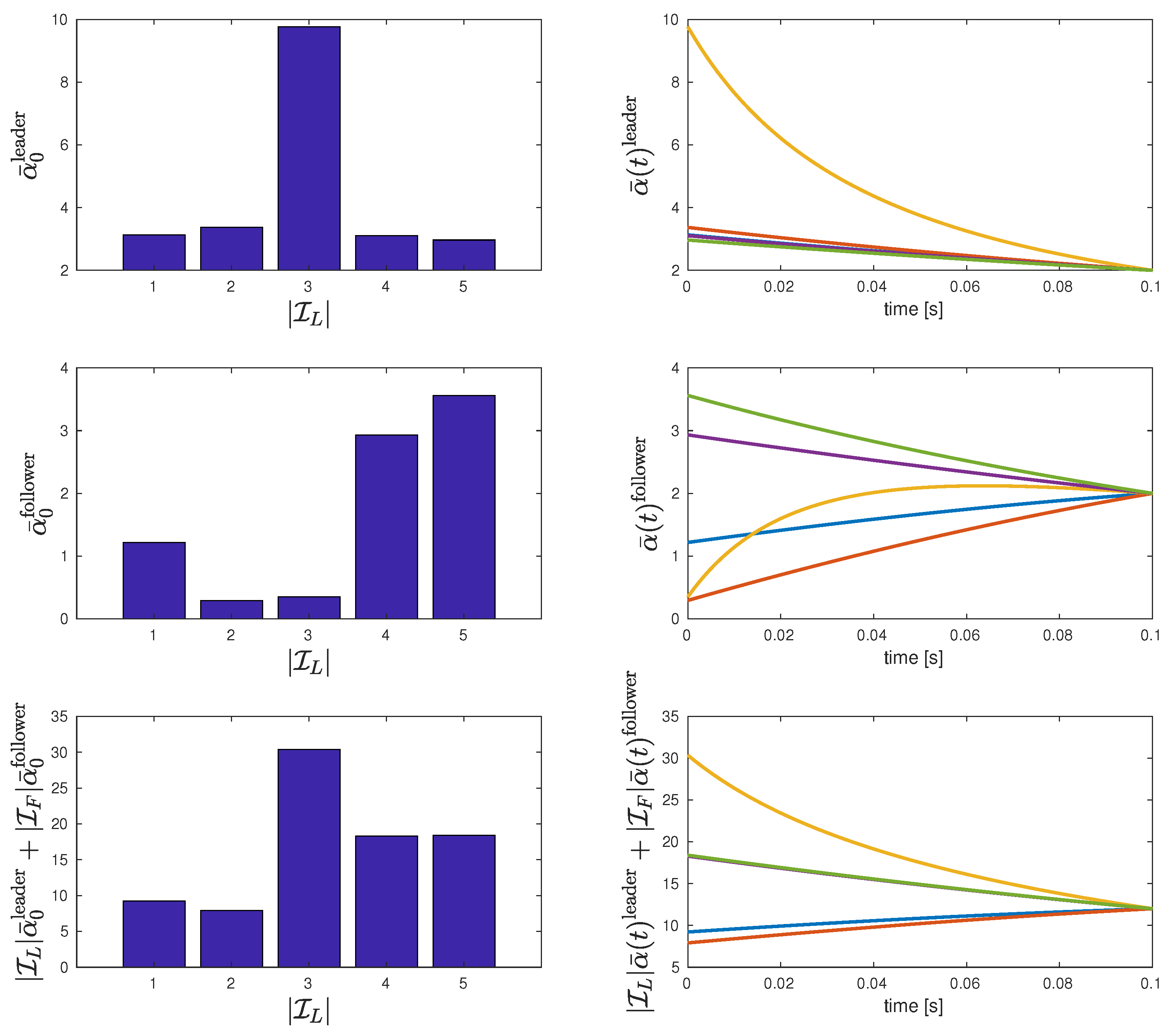
We numerically investigate $S\left(\right|{\mathcal{I}}_L|,{\delta }_{x_0})$ as a function of $\chi =|{\mathcal{I}}_L|$ for $\left|\mathcal{I}\right|=6.$ Let us consider a symmetric six-player game problem involving the parameters presented here:

$$\begin{array}{cccc}\hfill {\overline{c}}_i& =\overline{c}=0,\forall i\in \mathcal{I},\hfill & \hfill {\overline{k}}_i& =\overline{k}=1,\forall i\in \mathcal{I},\hfill \\ \hfill {\overline{ϵ}}_i& =\overline{ϵ}=1,\forall i\in \mathcal{I},\hfill & \hfill b_{2i}& =b_2=0.1,\forall i\in \mathcal{I},\hfill \\ \hfill {\overline{b}}_{2i}& ={\overline{b}}_2=0.5,\forall i\in \mathcal{I},\hfill & \hfill {\overline{r}}_i& =\overline{r}=2,\forall i\in \mathcal{I},\hfill \\ \hfill {\overline{q}}_i& =\overline{q}=1,\forall i\in \mathcal{I},\hfill & \hfill {\overline{q}}_{iT}& ={\overline{q}}_T=2,\forall i\in \mathcal{I},\hfill \\ \hfill T& =0.1.\hfill \end{array}$$

Figure 5 presents the evolution of both ${\dot{\overline{\alpha }}}^{\mathrm{leader}}$ and ${\dot{\overline{\alpha }}}^{\mathrm{follower}}$ for a different number of leaders $|{\mathcal{I}}_L|$. Notice that the initial values ${\overline{\alpha }}_0^{\mathrm{leader}}$ and ${\overline{\alpha }}_0^{\mathrm{follower}}$ determine the optimal cost considering that

$$\begin{array}{c}\hfill {\overline{x}}_0=\overline{x}\left(0\right)=\int ym(0,dy)=\int y{\delta }_{x_0}\left(dy\right)=x_0.\end{array}$$

(9)

Figure 5 and

Table 1. Summary of ${\overline{\alpha }}_0^{\mathrm{leader}}$, ${\overline{\alpha }}_0^{\mathrm{follower}}$, and $S\left(\right|{\mathcal{I}}_L|,{\delta }_{x_0})$ for the different number of leaders in the homogeneous scenario. bold—significant difference.

Leader(s)-Follower(s) Structure
Individual leader cost	3.132	3.37	9.772	3.107	2.968
Individual follower cost	1.217	0.2931	0.3481	2.933	3.562
Total cost	9.219	7.911	30.36	18.29	18.4

also show that, under the considered parameters, the lowest total cost is obtained when $|{\mathcal{I}}_L|=2,$ corresponding to a cost $S\left(\right|{\mathcal{I}}_L|,{\delta }_{x_0})=7.911$. These results offer an insight into the game’s structural design for the sake of either individual or total costs. We observe that having only one leader is suboptimal for the total cost. Having too many leaders (where the majority of the decision-makers are leaders) is not suboptimal for the total cost. In this setting, there is a tradeoff between leaders and followers, so that the system’s cost gets balanced.

6.1.2. Uniform Coupling and Heterogeneous Players

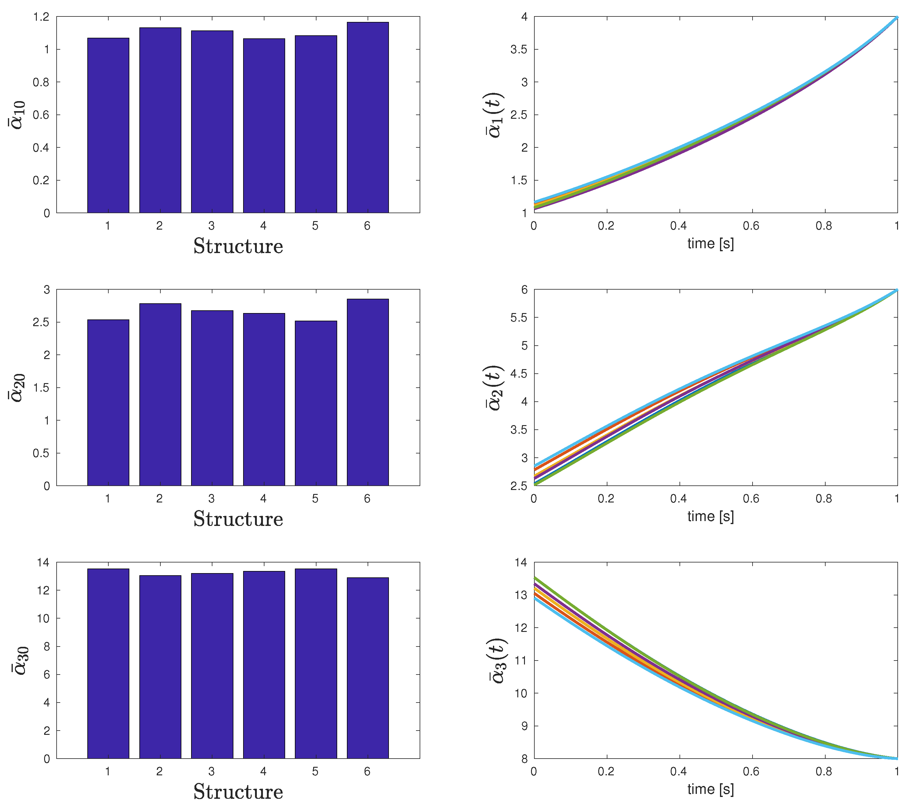
Now we investigate the two-layer case with uniform coupling, that is, ${\overline{ϵ}}_{ij}=0.1$, for all combinations $i,j\in \mathcal{I}$ and for the heterogeneous case with $\left|\mathcal{I}\right|=3$. We consider the following parameters:

$$\begin{array}{cccccc}\hfill b_{21}& =0.1,\hfill & \hfill b_{22}& =0.2,\hfill & \hfill b_{23}& =0.3,\hfill \\ \hfill {\overline{b}}_{21}& =0.5,\hfill & \hfill {\overline{b}}_{22}& =0.6,\hfill & \hfill {\overline{b}}_{23}& =0.7,\hfill \\ \hfill {\overline{r}}_1& =2,\hfill & \hfill {\overline{r}}_2& =2.1,\hfill & \hfill {\overline{r}}_3& =2.2,\hfill \\ \hfill {\overline{q}}_1& =1,\hfill & \hfill {\overline{q}}_2& =2,\hfill & \hfill {\overline{q}}_3& =3,\hfill \\ \hfill {\overline{q}}_{1T}& =4,\hfill & \hfill {\overline{q}}_{2T}& =6,\hfill & \hfill {\overline{q}}_{3T}& =8,\hfill \\ \hfill {\overline{b}}_1& =2,\hfill & \hfill T& =1,\hfill & \hfill {\overline{k}}_i& =\overline{k}=1,\forall i\in \mathcal{I},\hfill \end{array}$$

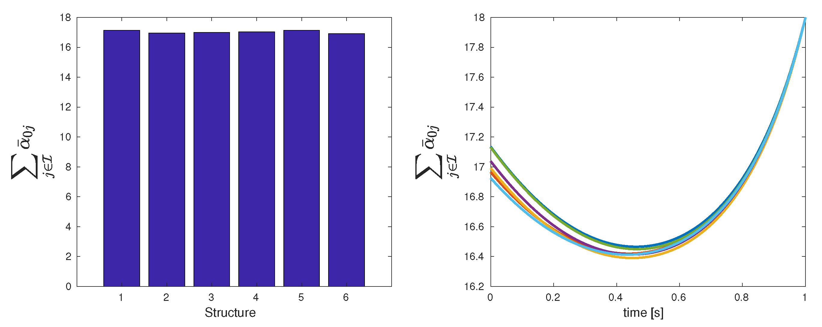
Figure 6 shows the evolution of ${\overline{\alpha }}_1,{\overline{\alpha }}_2,$ and ${\overline{\alpha }}_3$ for the different topologies presented in

Table 2. Summary of ${\overline{\alpha }}_0^{\mathrm{leader}}$, ${\overline{\alpha }}_0^{\mathrm{follower}}$, and $S\left(\right|{\mathcal{I}}_L|,{\delta }_{x_0})$ for the different number of leaders in the heterogeneous scenario. bold—significant difference.

Leader(s)-Follower(s) Structure
Leaders	$\left\{1\right\}\left\{2\right\}$	$\left\{1\right\}\left\{3\right\}$	$\left\{2\right\}\left\{3\right\}$	$\left\{1\right\}$	$\left\{2\right\}$	$\left\{3\right\}$
Followers	$\left\{3\right\}$	$\left\{2\right\}$	$\left\{1\right\}$	$\left\{2\right\}\left\{3\right\}$	$\left\{1\right\}\left\{3\right\}$	$\left\{1\right\}\left\{2\right\}$
Total cost	17.14	16.96	16.99	17.04	17.13	16.92

. It can be seen in Figure 7 that all the structures return a close value for the total cost. However, Table 2 shows that the best topology is the last one, where the third player acts as the unique leader assuming an initial condition, such that (10) holds.

6.2. Impact of the Hierarchical Structures

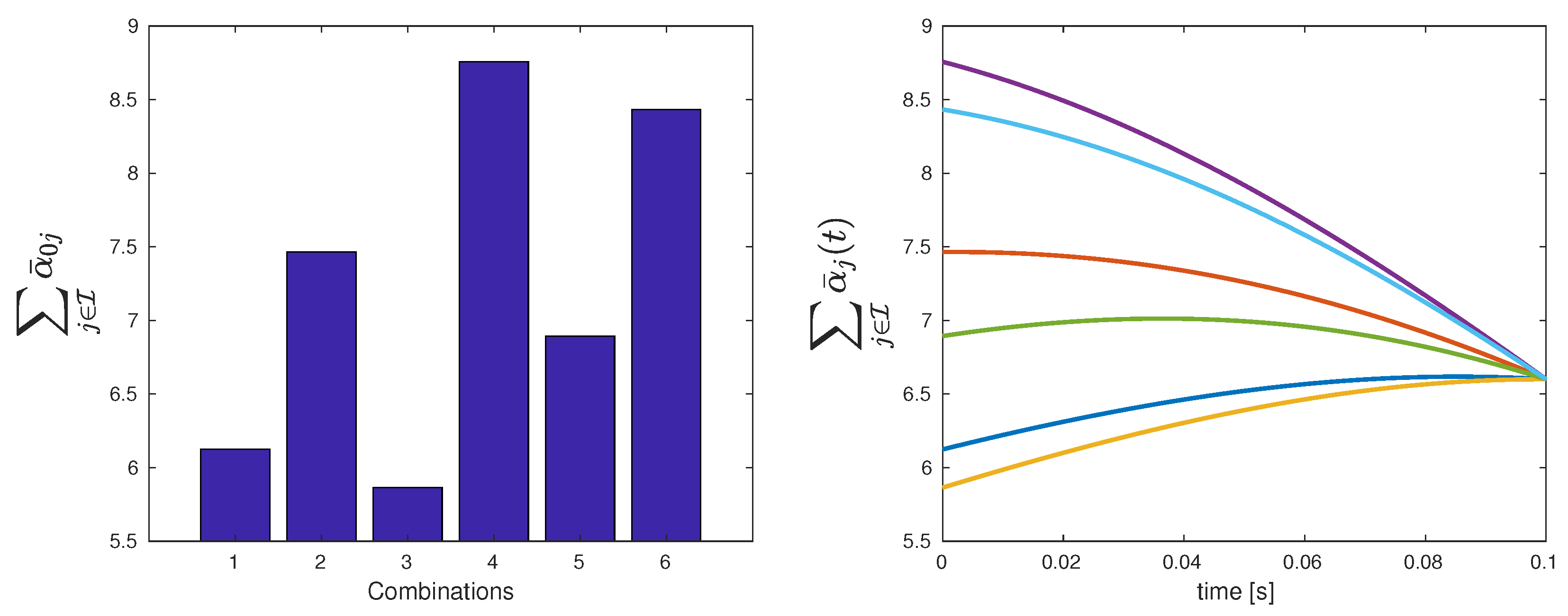
Here, we analyze the impact on the order of the strategic selection, that is, the hierarchical order on the heterogeneous case with $\left|\mathcal{I}\right|=3$. We consider the following heterogeneous parameters:

$$\begin{array}{cccccc}\hfill b_{21}& =0.1,\hfill & \hfill b_{22}& =0.2,\hfill & \hfill b_{23}& =0.3,\hfill \\ \hfill {\overline{b}}_{21}& =0.4,\hfill & \hfill {\overline{b}}_{22}& =0.5,\hfill & \hfill {\overline{b}}_{23}& =0.6,\hfill \\ \hfill {\overline{r}}_1& =1,\hfill & \hfill {\overline{r}}_2& =2,\hfill & \hfill {\overline{r}}_3& =3,\hfill \\ \hfill {\overline{q}}_1& =1.1,\hfill & \hfill {\overline{q}}_2& =1.2,\hfill & \hfill {\overline{q}}_3& =1.3,\hfill \\ \hfill {\overline{q}}_{1T}& =2.1,\hfill & \hfill {\overline{q}}_{2T}& =2.2,\hfill & \hfill {\overline{q}}_{3T}& =2.3,\hfill \\ \hfill {\overline{b}}_1& =2,\hfill & \hfill T& =0.1,\hfill & \hfill {\overline{k}}_i& =\overline{k}=1,\forall i\in \mathcal{I},\hfill \end{array}$$

and

$$\begin{array}{c}\hfill \overline{ϵ}=\left(\begin{array}{ccc}1& 1.2& 1.1\\ 1.5& 1& 1.6\\ 1.3& 1.4& 1\end{array}\right).\end{array}$$

Table 3. Total cost for the different hierarchical orders in a three-player case in the heterogeneous scenario. bold—significant difference.

Hierarchical Structure
Combination label	1	2	3	4	5	6
Hierarchical order	$\left\{1\right\}\left\{2\right\}\left\{3\right\}$	$\left\{1\right\}\left\{3\right\}\left\{2\right\}$	$\left\{2\right\}\left\{1\right\}\left\{3\right\}$	$\left\{2\right\}\left\{3\right\}\left\{1\right\}$	$\left\{3\right\}\left\{1\right\}\left\{2\right\}$	$\left\{3\right\}\left\{2\right\}\left\{1\right\}$
Total cost	6.124	7.464	5.864	8.757	6.894	8.433

shows the summary of the total costs for the six different possible hierarchical orders assuming an initial condition, such that (10) holds. It can be seen that the third configuration is the best to minimize the total cost. Moreover, Figure 8 presents the evolution of the equations ${\sum }_{j\in \mathcal{I}}{\dot{\overline{\alpha }}}_j\left(t\right)$ for all the possible structures.

7. Conclusions

In this paper, we have examined multi-layer hierarchical mean-field-type games with non-quadratic polynomial costs. We derived hierarchical mean-field-type solutions in linear state- and mean-field feedback form by using a partial integro-differential system, and also established the relationship between the Nash and the hierarchical solutions. Furthermore, we studied the impact of the number of leaders on a bi-level Stackelberg problem for both symmetric and non-symmetric scenarios. In addition, we have shown that the number of layers, permutations of the decision-makers per layer, and their identity significantly affect the total cost of the system. We have also numerically shown that the ordering among all permutations of heterogenous decision-makers may reduce the cost by a significant proportion, depending on the horizon. One open question that we leave for future investigation is to find, theoretically, the optimal ordering among all permutations of heterogenous decision-makers, and to examine the benefits/costs of structure design and leadership.

References

- Stackelberg, H.V. The Theory of the Market Economy; Peacock, A.J.; Hodge, W., Translators; Originally Published as Grundlagen der Theoretischen Volkswirtschaftlehre; Oxford University Press: Oxford, UK, 1948. [Google Scholar]
- Simaan, M.; Cruz, J.B. On the Stackelberg strategy in nonzero-sum games. J. Optim. Theory Appl. 1973, 11, 533–555. [Google Scholar] [CrossRef]
- Bagchi, A.; Basar, T. Stackelberg strategies in linear-quadratic stochastic differential games. J. Optim. Theory Appl. 1981, 35, 443–464. [Google Scholar] [CrossRef]
- Bensoussan, A.; Chen, S.; Sethi, S.P. The maximum principle for global solutions of stochastic Stackelberg differential games. SIAM J. Control Optim. 2015, 53, 1956–1981. [Google Scholar] [CrossRef]
- Pan, L.; Yong, J. A differential game with multi-level of hierarchy. J. Math. Anal. Appl. 1991, 161, 522–544. [Google Scholar] [CrossRef] [Green Version]
- Simaan, M.; Cruz, J. A Stackelberg solution for games with many players. IEEE Trans. Autom. Control 1973, 18, 322–324. [Google Scholar] [CrossRef]
- Cruz, J. Leader-follower strategies for multilevel systems. IEEE Trans. Autom. Control 1978, 23, 244–255. [Google Scholar] [CrossRef] [Green Version]
- Gardner, B.; Cruz, J. Feedback Stackelberg strategy for M-level hierarchical games. IEEE Trans. Autom. Control 1978, 23, 489–491. [Google Scholar] [CrossRef]
- Basar, T.; Selbuz, H. Closed-loop Stackelberg strategies with applications in the optimal control of multilevel systems. IEEE Trans. Autom. Control 1979, 24, 166–179. [Google Scholar] [CrossRef]
- Lin, Y.; Jiang, X.; Zhang, W. An Open-Loop Stackelberg Strategy for the Linear Quadratic Mean-Field Stochastic Differential Game. IEEE Trans. Autom. Control 2019, 64, 97–110. [Google Scholar] [CrossRef]
- Du, K.; Wu, Z. Linear-Quadratic Stackelberg Game for Mean-Field Backward Stochastic Differential System and Application. Math. Probl. Eng. 2019, 2019, 1798585. [Google Scholar] [CrossRef] [Green Version]
- Moon, J.; Basar, T. Linear-quadratic stochastic differential Stackelberg games with a high population of followers. In Proceedings of the 54th IEEE Conference on Decision Control, Osaka, Japan, 15–18 December 2015; pp. 2270–2275. [Google Scholar]
- Bensoussan, A.; Chau, M.H.M.; Yam, S.C.P. Mean-field Stackelberg games: Aggregation of delayed instructions. SIAM J. Control Optim. 2015, 53, 2237–2266. [Google Scholar] [CrossRef] [Green Version]
- Bensoussan, A.; Chau, M.; Lai, Y.; Yam, S. Linear-quadratic mean field Stackelberg games with state and control delays. SIAM J. Control Optim. 2017, 55, 2748–2781. [Google Scholar] [CrossRef]
- Averboukh, A.Y. Stackelberg solution for first-order mean-field game with a major player. Izv. Inst. Mat. Inform. Udmurt. 2018, 52. [Google Scholar] [CrossRef]
- Moon, J.; Basar, T. Linear quadratic mean field Stackelberg differential games. Automatica 2018, 97, 200–213. [Google Scholar] [CrossRef]
- Shi, J.; Wang, G.; Xiong, J. Leader-follower stochastic differential game with asymmetric information and applications. Automatica 2016, 63, 60–73. [Google Scholar] [CrossRef] [Green Version]
- Nourian, M.; Caines, P.; Malhamé, R.P.; Huang, M. Mean Field LQG Control in Leader-Follower Stochastic Multi-Agent Systems: Likelihood Ratio Based Adaptation. IEEE Trans. Autom. Control 2012, 57, 2801–2816. [Google Scholar] [CrossRef] [Green Version]
- Cai, H.; Hu, G. Distributed Tracking Control of an Interconnected Leader-Follower multi-agent System. IEEE Trans. Autom. Control 2017, 62, 3494–3501. [Google Scholar] [CrossRef]
- Li, Y.; Shi, D.; Chen, T. False Data Injection Attacks on Networked Control Systems: A Stackelberg Game Analysis. IEEE Trans. Autom. Control 2018, 63, 3503–3509. [Google Scholar] [CrossRef]
- Barreiro-Gomez, J.; Ocampo-Martinez, C.; Quijano, N. Partitioning for large-scale systems: A sequential distributed MPC design. In Proceedings of the 20th IFAC World Congress, Toulouse, France, 9–14 July 2017; pp. 8838–8843. [Google Scholar]
- Sutter, M.; Rivas, M.F. Leadership, Reward and Punishment in Sequential Public Goods Experiments. In Reward and Punishment in Social Dilemmas; Lange, P.A.V., Rockenbach, B., Yamagishi, T., Eds.; Oxford University Press: Oxford, UK, 2014; pp. 1–39. [Google Scholar]
- Andersson, D.; Djehiche, B. A Maximum Principle for SDEs of mean-field-type. Appl. Math. Optim. 2011, 63, 341–356. [Google Scholar] [CrossRef]
- Buckdahn, R.; Djehiche, B.; Li, J. A General Stochastic Maximum Principle for SDEs of mean-field-type. Appl. Math. Optim. 2011, 64, 197–216. [Google Scholar] [CrossRef]
- Tembine, H. Risk-sensitive mean-field-type games with Lp-norm drifts. Automatica 2015, 59, 224–237. [Google Scholar] [CrossRef]
- Tcheukam, A.; Tembine, H. mean-field-type Games for Distributed Power Networks in Presence of Prosumers. In Proceedings of the 2016 28th Chinese Control and Decision Conference (CCDC), Yinchuan, China, 28–30 May 2016; pp. 446–451. [Google Scholar]
- Djehiche, B.; Tcheukam, A.; Tembine, H. mean-field-type Games in Engineering. AIMS Electron. Electr. Eng. 2017, 1, 18. [Google Scholar] [CrossRef]
- Tembine, H. mean-field-type games. AIMS Math. 2017, 2, 706–735. [Google Scholar] [CrossRef]
- Duncan, T.; Tembine, H. Linear-Quadratic mean-field-type Games: A Direct Method. Games 2018, 9, 7. [Google Scholar] [CrossRef] [Green Version]
- Barreiro-Gomez, J.; Duncan, T.E.; Tembine, H. Linear-Quadratic mean-field-type Games: Jump-Diffusion Process with Regime Switching. IEEE Trans. Autom. Control 2019, 64, 4329–4336. [Google Scholar] [CrossRef]
- Barreiro-Gomez, J.; Duncan, T.E.; Tembine, H. Linear-Quadratic mean-field-type Games with Multiple Input Constraints. IEEE Control Syst. Lett. 2019, 3, 511–516. [Google Scholar] [CrossRef]
- Beardsley, X.W.; Field, B.; Xiao, M. Mean-variance-skewness-kurtosis portfolio optimization with return and liquidity. Commun. Math. Financ. 2012, 1, 13–49. [Google Scholar]
- Theodossiou, P.; Savva, C.S. Skewness and the Relation Between Risk and Return. Manag. Sci. 2016, 62, 1598–1609. [Google Scholar] [CrossRef] [Green Version]
- Sun, J.; Yong, J. Linear Quadratic Stochastic Differential Games: Open-Loop and Closed-Loop Saddle Points. SIAM J. Control. Optim. 2014, 52, 4082–4121. [Google Scholar] [CrossRef] [Green Version]
- Bensoussan, A.; Djehiche, B.; Tembine, H.; Yam, S.C.P. mean-field-type Games with Jump and Regime Switching. Dyn. Games Appl. 2020. [Google Scholar] [CrossRef]
Figure 1.
Different hierarchical designs and their solution concepts considered in this paper.
Figure 2.
Possible combinations in the hierarchical leadership design for two decision-makers. Ordered Bell number .
Figure 3.
Possible combinations in the hierarchical leadership design for three decision-makers. Ordered Bell number .
Figure 4.
Number of possible hierarchical structures for given set of decision-makers described by the ordered Bell number .
Figure 5.
Evolution of the differential equations , and the corresponding initial values for the different number of leaders in the homogeneous scenario.
Figure 6.
Evolution of the differential equations , and the corresponding initial values for the different number of leaders in the heterogeneous scenario.
Figure 7.
Evolution of the sum of differential equations and the corresponding total cost for the heterogeneous scenario.
Figure 8.
Evolution of the differential equations , and the corresponding initial values for different hierarchical structures in the heterogeneous scenario.