
A New Computational Algorithm for Assessing Overdispersion and Zero-Inflation in Machine Learning Count Models with Python


1
Faculty of Economics, Administration, Accounting and Actuarial Science, University of São Paulo, São Paulo 05508-010, Brazil
2
Polytechnic School, University of São Paulo, São Paulo 05508-010, Brazil
*
Author to whom correspondence should be addressed.
†
These authors contributed equally to this work.
Computers 2024, 13(4), 88; https://doi.org/10.3390/computers13040088
Submission received: 1 March 2024
/
Revised: 20 March 2024
/
Accepted: 24 March 2024
/
Published: 27 March 2024
Abstract
:This article provides an overview of count data and count models, explores zero inflation, introduces likelihood ratio tests, and explains how the Vuong test can be used as a model selection criterion for assessing overdispersion. The motivation of this work was to create a Vuong test implementation from scratch using the Python programming language. This implementation supports our objective of enhancing the accessibility and applicability of the Vuong test in real-world scenarios, providing a valuable contribution to the academic community, since Python did not have an implementation of this statistical test.
1. Introduction
Count data analysis is a statistical approach used to analyze data that consist of non-negative integer values, representing the number of occurrences of a specific event within a given context. This data type is commonly encountered in various fields, such as biology, economics, social sciences, and engineering. However, count data pose unique challenges due to their discrete nature, often exhibiting characteristics such as excessive zeros and overdispersion [1,2].
Excessive zeros refer to an unusually high number of observations with a count of zero, which cannot be adequately explained by standard statistical models. They require specialized techniques to be appropriately accounted for in the analysis to avoid biased model estimates [3,4,5]. Overdispersion occurs when the variance of the count data is higher than expected, indicating that additional sources of variation need to be accounted for beyond what the basic models can handle [2,6].
To address these complexities and effectively model count-based phenomena, specialized statistical models known as count models have been developed. Two commonly used count models are Poisson regression and negative binomial regression. Poisson regression is suitable for count data with low variability, assuming that the mean and variance of the data are equal. However, in cases where overdispersion is present, Poisson regression may not provide accurate results. Negative binomial regression, on the other hand, allows for overdispersion and provides a more flexible approach to model counts [7].
In this article, we aim to provide a comprehensive overview of count data analysis and count models. We explore the concept of zero inflation and its impact on count models, demonstrating how it can lead to model misspecification if not properly addressed. In addition, we introduce two statistical tests: the likelihood ratio test (LRT) and the Vuong test [8]. LRT is used to compare nested models and assess the improvement in model fit when additional parameters are added. On the other hand, the Vuong test is a model selection criterion that compares non-nested models, making it ideal for comparing count models with and without zero inflation.
Furthermore, the article emphasizes the practicality of our approach by providing the complete code we created that implements the Vuong test in the widely used Python programming language. Unlike R, which already has the function in the pscl package, and unlike STATA, which has the and functions, Python had no implementation of the Vuong test. Python is renowned for its ease of use and extensive libraries, making it an excellent choice for data analysts and researchers [9]. By creating a Python implementation of the Vuong test, we enhance the accessibility and applicability of this essential model selection technique in real-world scenarios, enabling readers to make informed model selection decisions and perform robust analysis of count-based phenomena in their projects.
2. Count Data
Count data refers to the observations made about events or items that are enumerated. More specifically, in the context of statistics, count data refers to the number of occurrences of an event within a fixed period. It only contains positive integer values that go from zero to some greater value, because an event cannot occur a negative number of times [1,3,10]. Examples of count data include the number of speeding tickets received in a year, the number of crimes on campus per semester, or the number of trips per year a person makes.
Following the concept of count data, it is possible to define a count variable as a list or array of count data [1]. Count variables indicate how many times something has happened, and can be used as response variables in statistical modeling when the goal is to understand or predict the factors influencing the count [3,11].
3. Count Models
In simple terms, a statistical model helps us understand how different variables are related to each other. It provides a mathematical representation of how one variable or a set of variables can explain or predict another variable. Specifically, when we have a count variable, the statistical model helps us explain the counts using one or more explanatory variables [1,12].
Statistical models are considered stochastic because they are based on probability functions. This means that they take into account the uncertainty and variability inherent in real-world data. Instead of providing exact predictions or explanations, the model provides a probabilistic framework that describes the likelihood or probability of different outcomes [13]. By utilizing statistical models, we can analyze and quantify the relationships between variables, make predictions, and assess the statistical significance of explanatory factors. These models allow us to gain insights into the underlying patterns and processes driving the count variable, accounting for the inherent randomness and variability observed in real-world phenomena. With respect to count data, those statistical models have applications that exploit the full probability distribution of counts to provide comprehensive predictions. This capability enhances our ability to interpret and utilize count data effectively in various applications, such as forecasting, risk assessment, resource allocation, and decision-making [12].
When using count variables in ordinary least squares (OLS) regression, there are potential issues to consider. OLS regression, which has minimal assumptions about predictors, allows count variables to be used as predictors, with one caveat. If the count variable has very little variability, which can happen with count data having a small range, the regression coefficient associated with that predictor becomes unstable and has a large standard error [14]. It is important to note that this instability is not unique to count predictors—any predictor with low variability would result in an unstable regression coefficient.
However, different problems arise when a count variable is used as the outcome or dependent variable in OLS regression. When the average count value of the outcome variable is relatively high, OLS regression can generally be applied without significant difficulty. But when the mean of the outcome variable is low, OLS regression produces undesirable outcomes, including biased standard errors and significance tests [10].
So, while count variables can be used as predictors in OLS regression with caution, using count variables as outcome variables in OLS regression can result in inefficient, inconsistent, and biased estimates. Even though there are situations in which the linear regression model (LRM) provides reasonable results, it is much safer to employ regression models specifically designed for count outcomes, as they offer improved statistical power and appropriately handle the specific characteristics of count data [10,11]. Examples of such models include Poisson regression, negative binomial regression (NB), and variations of these models for zero-inflated counts (ZIP and ZINB). These models consider the discrete nature of count variables, their variability, and the specific statistical assumptions needed for accurate estimation and inference [6,11].
Generalized linear models offer a versatile method for addressing a wide variety of response modeling issues. The most frequently used responses are normal, Poisson, and binomial, but other distributions may also be employed [15,16]. When dealing with count data, we typically begin by estimating the parameters using a Poisson regression model because of its simplicity. In this scenario, the dependent variable in a Poisson regression model should adhere to a Poisson distribution with the mean equaling the variance [17]. However, this property is frequently violated in empirical research, as it is common for there to be overdispersion, where the variance of the dependent variable exceeds its mean. In such instances, we will estimate a negative binomial regression model [2,18].
4. Poisson and Negative Binomial Models
The Poisson distribution is distinct from the normal distribution in several ways that make it more appealing for representing the characteristics of count data. Firstly, the Poisson distribution is a discrete distribution that only assumes probability values for non-negative integers. This feature of the Poisson distribution makes it an ideal choice for modeling count outcomes, which can only take on integer values of 0 or more [10]. The Poisson distribution, for a given observation i, has the following probability of occurrence of a count m (m = 0, 1, 2, …) in a given exposure:
In (1), is the expected number of occurrences or the estimated incidence rate ratio of the phenomenon under study for a given exposure. In the Poisson distribution, the mean and variance of the variable under study must be equal to . This characteristic is known as the equidispersion of the Poisson distribution. If this condition is satisfied, a Poisson regression model can be calculated, which is described as follows:
In (2), stands for the constant, (j = 1, 2, …, k) are the calculated parameters for each explanatory variable, are the explanatory variables (either metrics or dummies), and the subscript i denotes each observation in the sample (i = 1, 2, …, n, where n is the size of the sample).
The log-likelihood function, which must be maximized, can be written as:
As previously noted, the data are assumed to have equidispersion. If this is not the case, a negative binomial regression model could be used for estimation [1]. The NB distribution uses an additional parameter to model overdispersion. In other words, an NB-distributed random variable is equivalent to a Poisson random variable with a random, Gamma-distributed mean, allowing it to model unobserved individual heterogeneity [4].
For a given observation i (i = 1, 2, …, n, where n is the sample size), the probability distribution function of the variable will be given by the following:
In (4), is called the shape parameter (), is called the rate parameter () and, for and integer, can be approximated by . The log-likelihood function for the NB2 regression, which must be maximized, can be written as:
5. Zero-Inflated Count Data Models
Simply testing for overdispersion and using an NB model may not be enough. It is important to note that overdispersion can be caused by an excess of zeros in the data, and this zero inflation may need to be accounted for in the model [4,5].
When data are zero-inflated, it is necessary to modify the Poisson or NB procedure to prevent incorrect estimation of model parameters and standard errors, as well as incorrect specification of the distribution of test statistics. Ignoring these misspecifications can lead to incorrect conclusions about the data and introduce uncertainty into research and practice. As a result, the use of zero-inflated Poisson (ZIP) and zero-inflated negative binomial (ZINB) models has grown in popularity across a wide range of fields [22].
According to [23], zero-inflated regression models are considered a combination of a count data model and a binary data model. They are used to investigate the reasons for a certain number of occurrences (counts) of a phenomenon, as well as the reasons for the occurrence (or not) of the phenomenon itself, regardless of the number of counts observed.
Facing this scenario, according to [24], the first step is to address potential overdispersion in the distribution by comparing Poisson versus NB models, using statistical tests such as the likelihood ratio test (LRT) and the Wald test. The next step is to assess whether the distribution has an excess of zeros by comparing Poisson versus ZIP or NB versus ZINB models, using the Vuong test [8]. If the zero-inflated version of the model fits the data significantly better than the standard model, it is considered evidence that the data contain an excess of zeros [4].
5.1. Zero Inflated Poisson Models
In the ZIP model, the probability p of observing zero counts for a given observation i (, where n is the sample size), or , is determined by combining a dichotomous component with a count component. As a result, the probability of observing zero counts due solely to the dichotomous component must be established. The probability of observing a specific count m (), or , is determined by the probability expression of the Poisson distribution, multiplied by () [7]. To sum up, for , we have the following equations, on which ():
It is evident that if , the probability distribution in expression (6) simplifies to the Poisson distribution, even for instances where . In other words, ZIP regression models have two processes that generate zeros. One is due to the binary distribution, which generates what are known as structural zeros. The other is due to the Poisson distribution, which generates count data, including what is known as sample zeros [7].
The log-likelihood function of a ZIP regression model (7) should also be maximized.
5.2. Zero-Inflated Negative Binomial Models
In the ZINB models, The probability of no counts for a given observation i, or , is also calculated by adding a dichotomous component to a count component. The chance of a specific count m (), or , now follows the probability expression of the Poisson-Gamma distribution [7]. In Equation (8), for , (), represents the inverse of the shape parameter of a given Gamma distribution.
The log-likelihood function of a ZINB regression model (9) should also be maximized.
6. Likelihood Ratio Tests for Model Selection: Vuong Test
The decision to use either conventional count regression or zero-inflated modeling is based on the balance between avoiding overfitting and accurately representing the empirical features of the data. One way to determine if a zero-inflated model is necessary is to compare its fit to that of a standard count model. This test is important because choosing the wrong model can have consequences. If the standard model is chosen when the zero-inflated model is more appropriate, an important part of the data-generating process may be overlooked. On the other hand, if the zero-inflated model is chosen when it is not necessary, the model becomes unnecessarily complicated by adding an extra equation [25,26,27,28,29].
With this dilemma in mind, researchers commonly use the Vuong test [8] to determine whether the zero-inflated model fits the data statistically significantly better than count regression with a single equation. The Vuong test is a method for comparing the fit of two models to the same data using maximum likelihood. Its purpose is to test the null hypothesis that the two models fit the data equally well. The models being compared need not be nested, and one of them does not need to be the correct specification [25,26,27,28,29].
7. Vuong Test Implementation on Python
Python is currently experiencing a surge in popularity as a programming language, and this can be attributed to several factors. Firstly, Python is known for its ease of use and accessibility, making it an attractive option for beginners. Additionally, the learning curve for Python is relatively fast, allowing new users to quickly become proficient. Another major draw for Python is the vast array of high-quality packages available for data science and machine learning applications.
Several libraries in Python already support statistical and econometric analysis, such as statsmodels [30] and pandas [31]. However, when it comes to general statistics, Python lags behind the R programming language. As a result, many scientists continue to rely on R for their statistical analysis [32].
In an effort to make Python more complete for statistical analysis, a gap was identified in the Vuong test, which currently lacks an implementation in Python. So, we present a code that implements the Vuong test in Python. In addition, we demonstrate its use on a database [33]. Other machine learning and deep learning studies have already been covered in the same journal, such as [34,35,36].
7.1. Corruption Database
According to [33], in an empirical approach developed for evaluating the role of both social norms and legal enforcement in corruption by studying parking violations among United Nations diplomats living in New York City, diplomatic immunity is a privilege that allows mission personnel and their families to avoid paying parking fines. This was the case until November 2002. Illegal parking can be considered an act of corruption, as it is an abuse of power for personal gain. Comparing parking violations by diplomats from different societies can serve as a measure of the extent of corruption norms or culture.
The data set contains the following information:
- Country name
- Code of the country
- Number of parking violations
- Number of UN Mission diplomats in 1998
- Indicator (Yes/No) that the data are before or after the law enforcement
- Corruption Index (CI) [37]
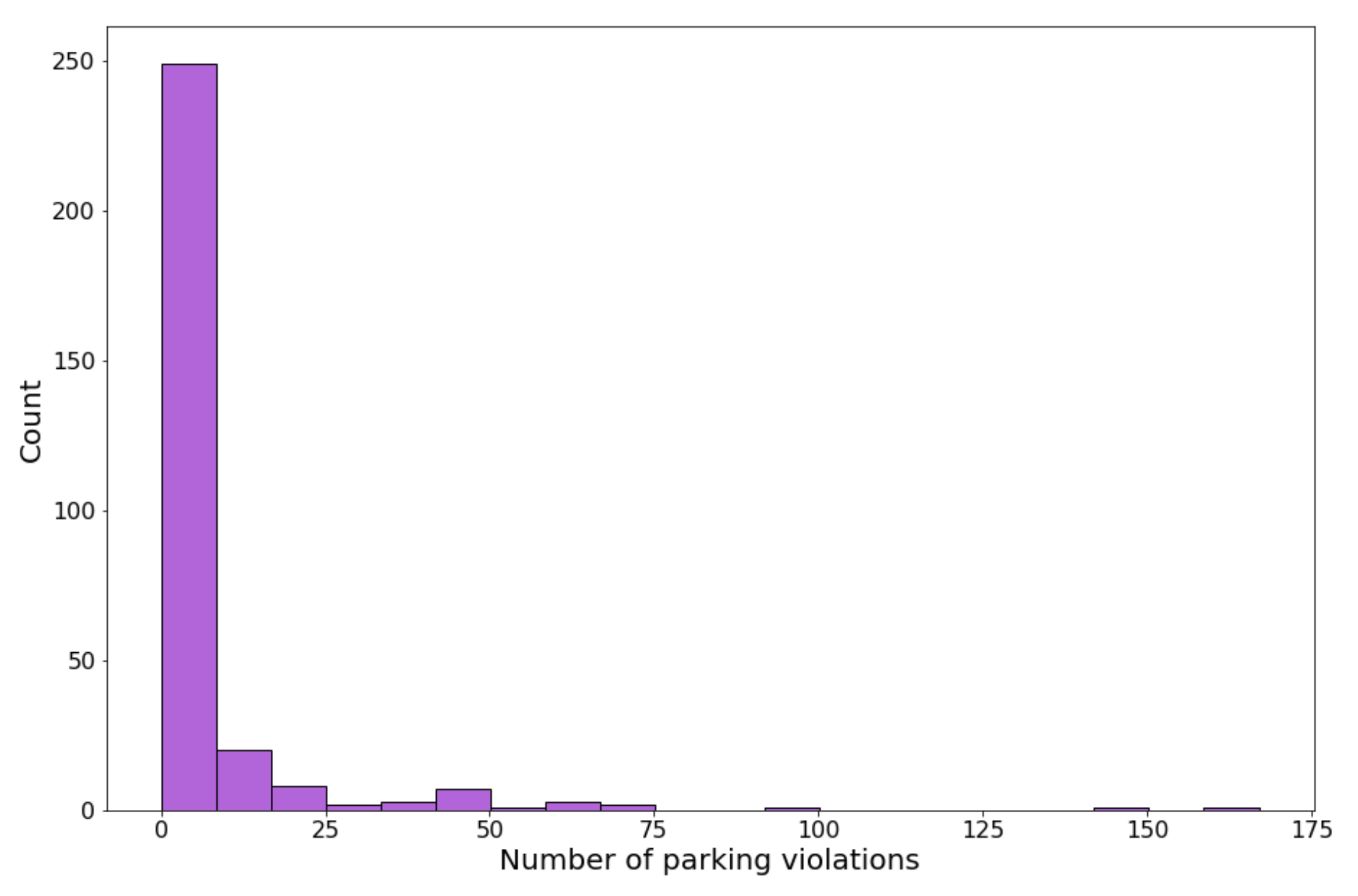
The data set is organized in a table as presented in Table 1. It contains data from 149 countries, and it has 298 rows, with each country having two rows (one for data before law enforcement and the other for after law enforcement). Also, the histogram of the data (counts per number of parking violations) is shown in Figure 1.
7.2. Code Availability
The Python code that was developed to implement the Vuong test [8] is available in Appendix A-Code. It is important to execute the following command before running the code to update the statsmodel version required.
7.3. Computational Environment and Analysis Setup
The analysis was conducted on a notebook equipped with an Intel Core i5-1235U processor (1.30 GHz, 12 cores, 12 threads), 20 GB of DDR4 RAM, and an Intel IRIS Xe graphics card. The computer ran Windows 11 as the operating system. Analysis was performed using Python 3.11.3 with libraries including NumPy 1.26.3, pandas 2.2.0, statsmodels 0.14.1, and scipy 1.12.0. No parallelization was utilized, as the algorithm ran efficiently on a single processor.
7.4. Efficiency and Performance of the Algorithm
The algorithm employed in this study is not computationally demanding, as evidenced by its smooth execution and negligible runtime. It ran effortlessly on the available hardware, completing its tasks in a remarkably short amount of time.
8. Results
First, a preliminary diagnosis of equidispersion was elaborated (observation of possible equality between the mean and the variance of the dependent variable ‘violations’). As can be seen in Table 2, the mean () and the variance () are very distant from each other. Therefore, there is a preliminary indication of overdispersion.
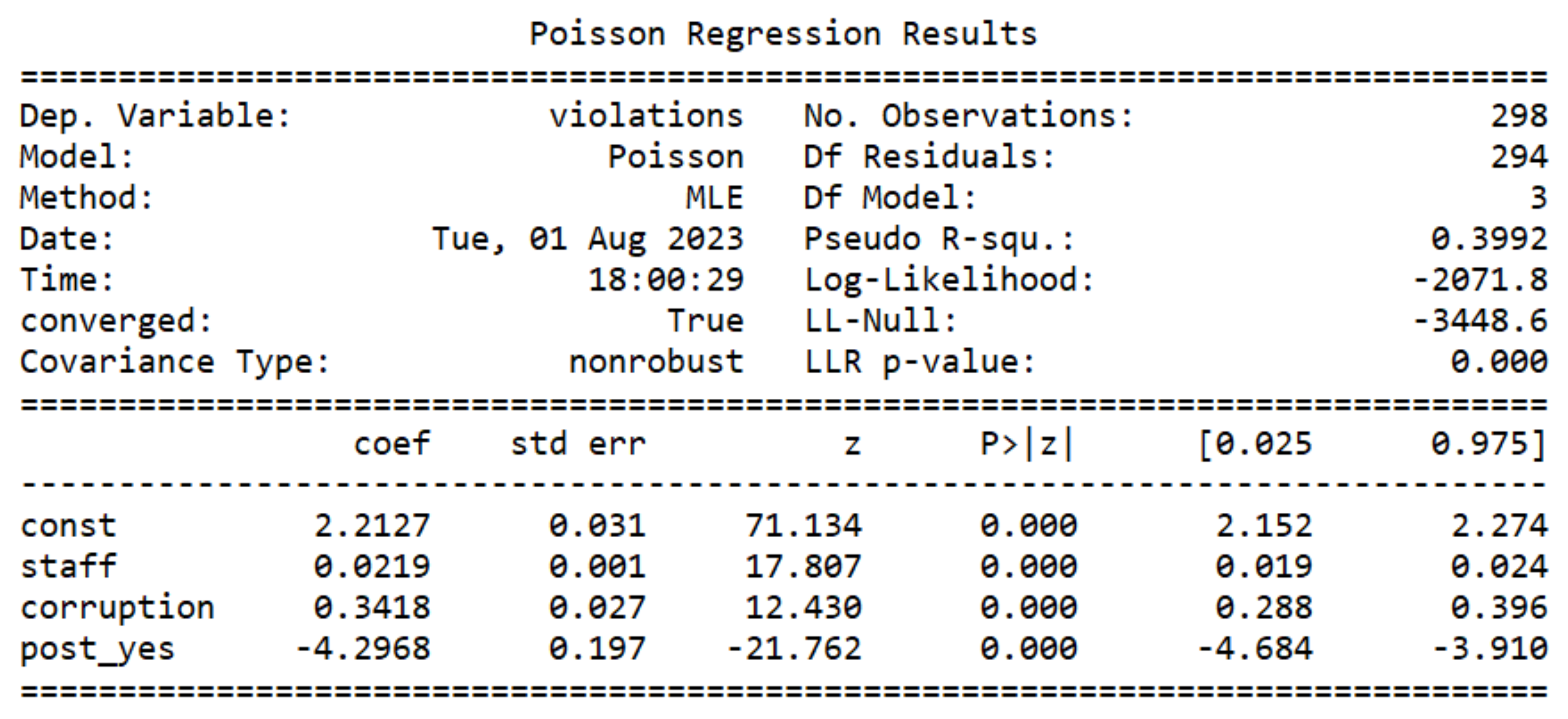
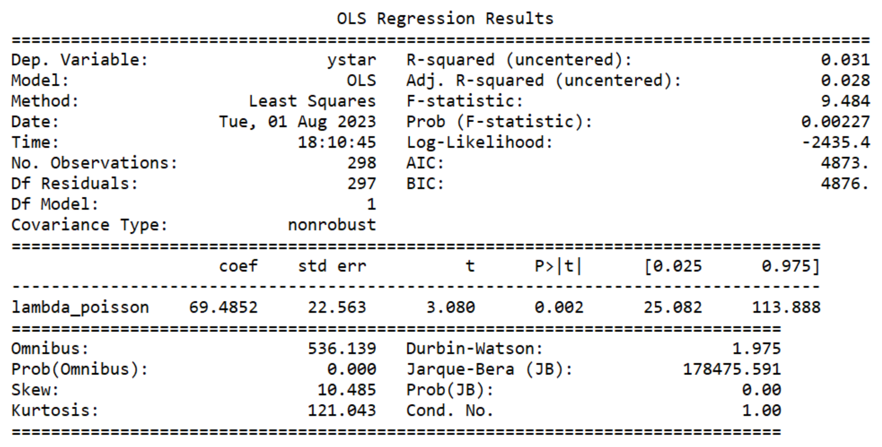
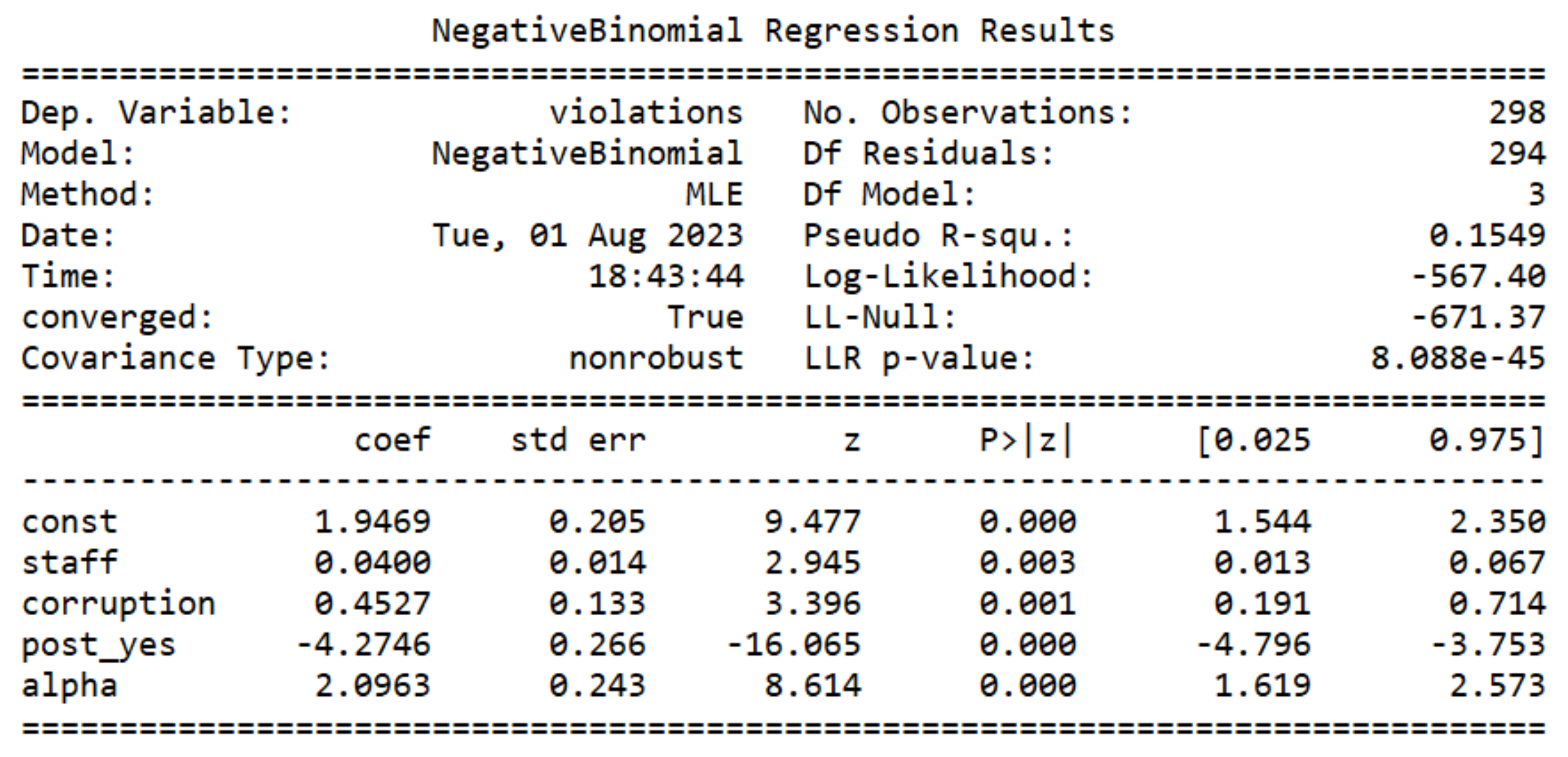
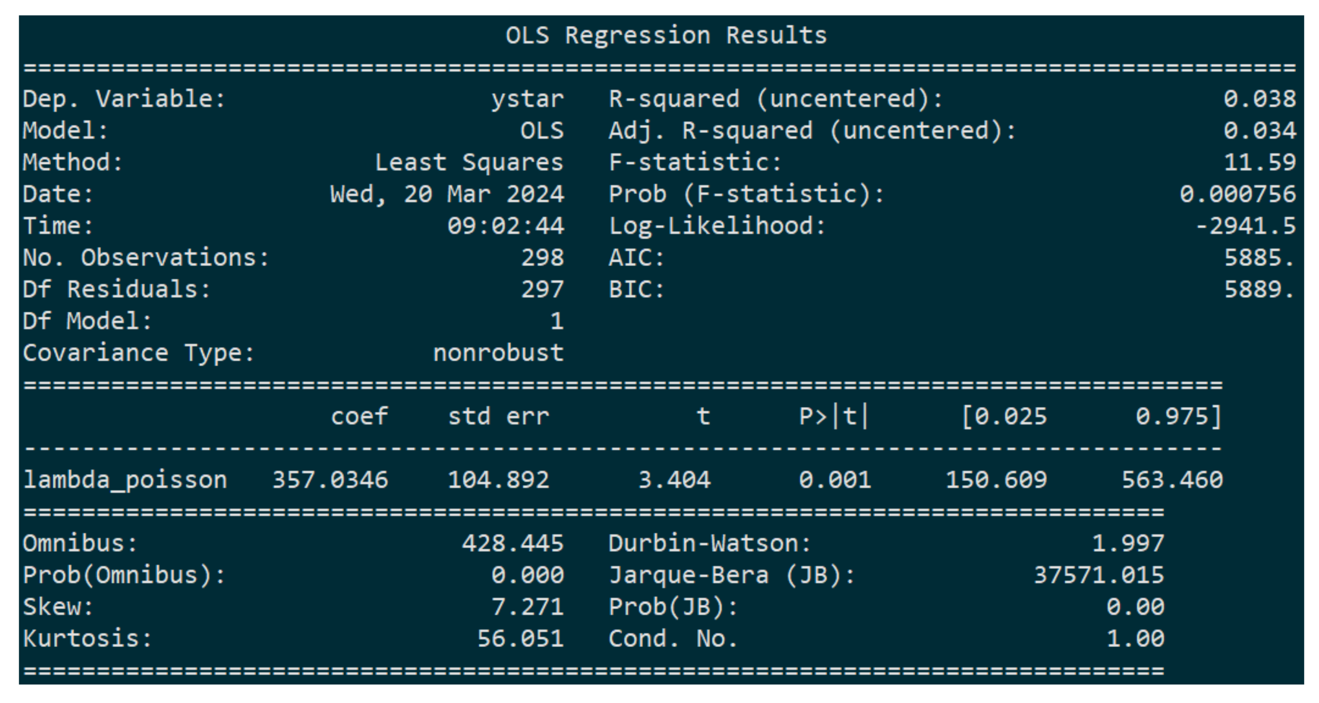
The next step was to estimate the Poisson model, as can be seen in Figure 2. Then, it was tested whether the data exhibited equidispersion [38]. The test can be seen in Figure 3. As the p-value of the t-test corresponding to the parameter of is less than 0.05, with a value of 0.02, it can be stated that the data of the dependent variable present overdispersion, making the estimated Poisson regression model inadequate. Then, we proceed to estimate the negative binomial model, as can be seen in Figure 4.
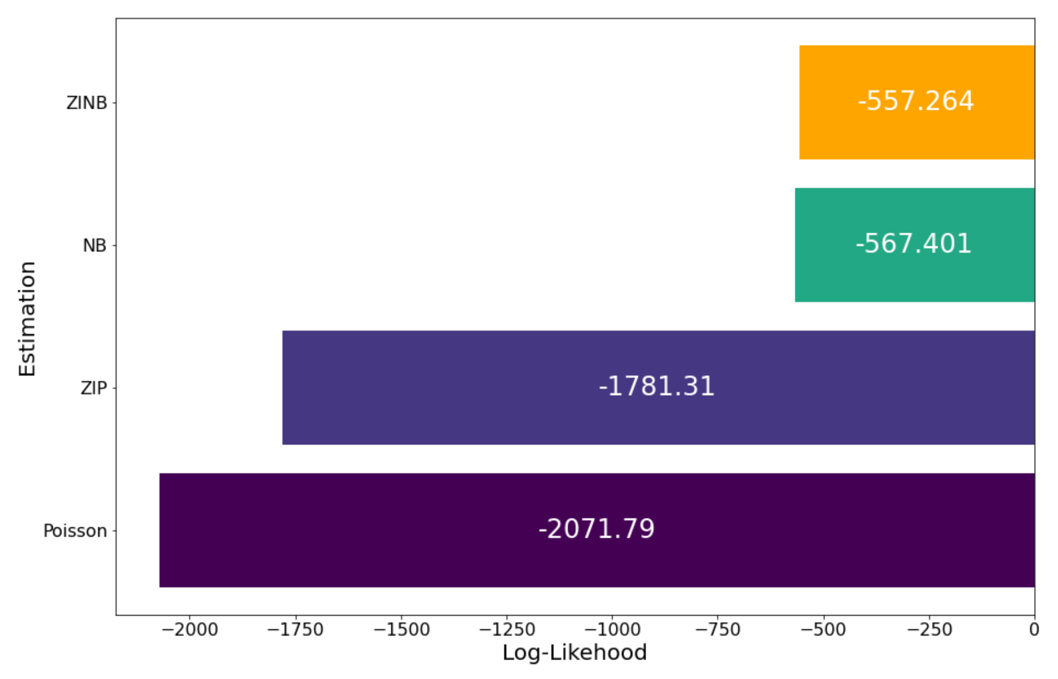
By comparing the log-likelihood (LL) of the Poisson (Equation (3)) and negative binomial models (Equation (5)), as shown in Figure 2 and Figure 4, we can see that the NB has a smaller LL than the Poisson. The log-likelihood is close to −567.4 for the NB model, and close to −2071.79 for the Poisson model.
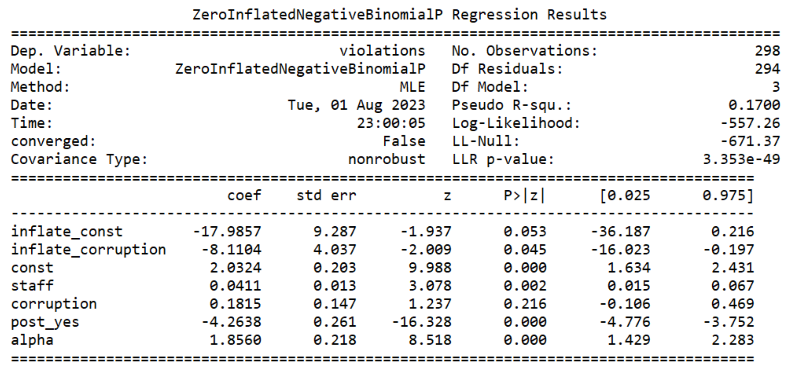
The next step is to estimate the zero-inflated Poisson model and the zero-inflated NB model, which can be seen in Figure 5 and Figure 6, respectively.
By comparing the log-likelihood (LL) of the ZIP (Equation (7)) and ZINB (Equation (9)) models, it is possible to see, in Figure 7, that the ZINB has a smaller LL than ZIP. The log-likelihood (LL) is close to −557.26 for the ZINB model, and close to −1781.31 for the ZIP model.
After analyzing all the models regarding log-likelihood (LL), as can be seen in Figure 7, it is possible to determine that the ZINB model is the best, considering that its LL is the highest among all models.
After that, it is possible to apply the Vuong test that was developed to compare the Poisson model (Figure 2) with the ZIP model (Figure 5) and to compare the NB model (Figure 4) with the ZINB model (Figure 6).
The algorithm performs some checks, such as making sure that only the ZIP, ZINB, Poisson, and negative binomial models are being used in the function. Other checks include ensuring that the dependent variables have the same number of observations and ensuring that the dependent variables have the same values. Finally, the developed algorithm follows the step-by-step process below:
- Extracts the dependent variables (y) from each model.
- Calculates the logarithms of the predicted probabilities for each model.
- Calculates the difference between the logarithms of the predicted probabilities of both models.
- Calculates the z-statistic of Vuong’s hypothesis test.
- Calculates the p-value associated with Vuong’s hypothesis test.
- Prints the hypothesis test value (z-statistic) and the p-value.
The code returns the outputs in Table 3.
9. Discussion
In the Vuong test, positive and statistically significant values indicate the adequacy of the ZIP or ZINB model. Negative and statistically significant values indicate the adequacy of the traditional Poisson model or negative binomial model [7].
As previously discussed, the data are overdispersed, making the estimated Poisson model inadequate. In this case, the Vuong test is used to choose between the NB model and the ZINB model. Considering that the Vuong test resulted in , with a p-value (Table 3), the traditional NB model is a better option than the ZINB at a significance level of 95%.
In Figure 8, a comparison of the models is shown. It includes the observed, predicted, and fitted values, and the confidence intervals for Poisson, NB, ZIP, and ZINB. The fitted values are different for each estimation. The NB and ZINB models are able to adjust better to higher values of the y variable, which demonstrates their ability to estimate parameters that exhibit long-tail behavior (overdispersion).
In terms of robustness and sensitivity analysis, the results discussed were obtained considering a data set with 156 zeros among a total of 298 values for the variable ‘violations’, as can be seen in the histogram in Figure 1. This would already represent a very imbalanced data set, considering that around 52% of the values are zeros. Also, our data set was relatively overdispersed, as can be seen in Table 2 and in Figure 3. We then sought to modify our sample to evaluate our algorithm in terms of robustness and sensitivity analysis. The following changes were made:
- We replaced the values 1 and 2 in ‘violations’ with zeros, increasing the number of zeros to 207 out of 298, which represents a percentage of approximately 69.5%.
When modifying the sample in the way shown, it can be seen that, in addition to the portion of zeros being much higher than for the initial set of data, there is also much more significant overdispersion, as can be seen in Appendix B, Figure A1. Repeating all the analyses performed for the original data set, we obtain the following output from the Vuong test, as can be seen in Table 5.
As previously discussed, the data are overdispersed, making the estimated Poisson model inadequate. In this case, the Vuong test is used to choose between the NB model and the ZINB model. Considering that the Vuong test resulted in −1.2879, with a p-value > 0.05 (Table 5), the ZINB model is a better option than the NB at a significance level of 95%. Therefore, in the modified data set, we find that the ZINB model is preferable to the NB model, the opposite of the output for the original data set.
Regarding the performance of the algorithm on different data sets, we tested it for other examples and realized that it maintains the accuracy of the results, only varying the computational time for larger data sets. For the initial data set (298 rows), the compilation time was practically instantaneous. For a data set with 100,000 rows, the compilation time was approximately 10 s. Finally, for a data set with 1,000,000 (one million) rows, the compilation time was approximately 5 min.
10. Conclusions
The motivation for our work was to provide a new computational algorithm, on Python, to assess overdispersion in machine learning models. In that sense, the objective for this article was to create an implementation of the Vuong test using Python, since to date, there was no implementation of this statistical test in this programming language, providing a valuable contribution to the academic community.
With the analysis developed in this paper, the newly developed algorithm has proven to be a useful tool for choosing between regular or zero-inflated models. The numerical results of the Vuong test algorithm, as can be seen in Table 3, provide a clear indicator of which model should be used (the one with the highest Vuong z-statistic value), with their respective p-values, indicating statistical significance.
Prior to our work, this test did not exist in the Python environment. Now, other researchers can benefit from our contribution by using the code we have made available in Appendix A of this paper to apply the Vuong test in their research using Python. We welcome any user feedback on the algorithm for future improvements.
While the existing methodology marks a notable achievement, there is potential value in investigating enhancements or alternative computational approaches to improve precision, velocity, or resilience. Future research may involve exploring parallel processing methodologies or utilizing advancements in machine learning frameworks.
Author Contributions
Conceptualization, L.P.L.F., A.D. and H.P.S.; Methodology, L.P.L.F., A.D. and H.P.S.; Software, L.P.L.F., A.D. and H.P.S.; Validation, L.P.L.F. and A.D.; Formal analysis, A.D. and H.P.S.; Investigation, A.D.; Data curation, A.D.; Writing—original draft, A.D.; Writing—review & editing, L.P.L.F. and A.D.; Supervision, L.P.L.F.; Project administration, L.P.L.F. All authors have read and agreed to the published version of the manuscript.
Funding
This research received no external funding.
Data Availability Statement
The full code and the data that were used to generate tables, graphs, histograms, and the Vuong test are available on GitHub (see https://github.com/DuarteAlexandre/VuongTest.git, accessed on 29 February 2024).
Acknowledgments
The following AI-assisted tools were used in this paper: DeepL Write (AI-based writing assistant) and Grammarly (AI writing assistance). Both of those tools were used to structure the text better, with sentences that make more sense and are more cohesive.
Conflicts of Interest
The authors declare no conflicts ofinterest.
Abbreviations
The following abbreviations are used in this manuscript:
| ZIP | Zero-Inflated Poisson |
| ZINB | Zero-Inflated Negative Binomial |
| LRT | Likelihood Ration Tests |
| OLS | Ordinary Least Squares |
| NB | Negative Binomial |
| LL | Log-Likelihood |
| CI | Confidence Interval |
Appendix A. Vuong Test Code in Python
def vuong_test (m1, m2):

    from statsmodels.discrete.count_model import
        ZeroInflatedPoisson, ZeroInflatedNegativeBinomialP
    from statsmodels.discrete.discrete_model import Poisson,
        NegativeBinomial
    from scipy.stats import norm

    supported_models = [ZeroInflatedPoisson,
                      ZeroInflatedNegativeBinomialP,
                      Poisson,
                      NegativeBinomial]

    if type (m1.model) not in supported_models:
        raise ValueError (f"Model type not supported for first
            parameter. List of supported models:
            (ZeroInflatedPoisson, ZeroInflatedNegativeBinomialP,
            Poisson, NegativeBinomial) from statsmodels discrete
            collection.")

    if type (m2.model) not in supported_models:
        raise ValueError (f"Model type not supported for second
            parameter. List of supported models:
            (ZeroInflatedPoisson, ZeroInflatedNegativeBinomialP,
            Poisson, NegativeBinomial) from statsmodels discrete
            collection.")

    m1_y = m1.model.endog
    m2_y = m2.model.endog

    m1_n = len(m1_y)
    m2_n = len(m2_y)

    if m1_n == 0 or m2_n == 0:
        raise ValueError ("Could not extract dependent variables from
            models.")

    if m1_n != m2_n:
        raise ValueError ("Models appear to have different numbers of
            observations.\n"
                         f"Model 1 has {m1_n} observations.\n"
                         f"Model 2 has {m2_n} observations.")

    if np.any(m1_y != m2_y):
        raise ValueError ("Models appear to have different values on
            dependent variables.")

    m1_linpred = pd.DataFrame (m1.predict (which ="prob"))
    m2_linpred = pd.DataFrame (m2.predict (which ="prob"))

    m1_probs = np.repeat (np.nan, m1_n)
    m2_probs = np.repeat (np.nan, m2_n)

    which_col_m1 = [list (m1_linpred.columns).index (x) if x in
        list (m1_linpred.columns) else None for x in m1_y]
    which_col_m2 = [list(m2_linpred.columns).index (x) if x in
        list(m2_linpred.columns) else None for x in m2_y]

    for i, v in enumerate (m1_probs):
        m1_probs [i] = m1_linpred.iloc [i, which_col_m1[i]]

    for i, v in enumerate (m2_probs):
        m2_probs [i] = m2_linpred.iloc [i, which_col_m2[i]]

    lm1p = np.log(m1_probs)
    lm2p = np.log(m2_probs)

    m = lm1p - lm2p

    v = np.sum(m) / (np.std (m) * np.sqrt(len(m)))

    pval = 1 - norm.cdf(v) if v > 0 else norm.cdf(v)

    print ("Vuong Non - Nested Hypothesis Test - Statistic (Raw):")
    print (f"Vuong z- statistic: {v}")
    print (f"p-value: {pval}")
Appendix B. Equidispersion Test for the Modified Data Set
Figure A1.
Equidispersion test for the modified data set.

References
- Hilbe, J.M. Modeling Count Data; Cambridge University Press: Cambridge, UK, 2014. [Google Scholar]
- Payne, E.H.; Hardin, J.W.; Egede, L.E.; Ramakrishnan, V.; Selassie, A.; Gebregziabher, M. Approaches for dealing with various sources of overdispersion in modeling count data: Scale adjustment versus modeling. Stat. Methods Med. Res. 2017, 26, 1802–1823. [Google Scholar] [CrossRef] [PubMed]
- Cameron, A.C.; Trivedi, P.K. Essentials of Count Data Regression. In A Companion to Theoretical Econometrics; Wiley Online Library: Hoboken, NJ, USA, 2001; Volume 331. [Google Scholar]
- Winkelmann, R. Econometric Analysis of Count Data; Springer Science & Business Media: Berlin/Heidelberg, Germany, 2008. [Google Scholar]
- Atkins, D.C.; Gallop, R.J. Rethinking how family researchers model infrequent outcomes: A tutorial on count regression and zero-inflated models. J. Fam. Psychol. 2007, 21, 726. [Google Scholar] [CrossRef] [PubMed]
- Cameron, A.C.; Trivedi, P.K. Regression Analysis of Count Data; Cambridge University Press: Cambridge, UK, 2013. [Google Scholar]
- Fávero, L.P.; Belfiore, P. Manual de Análise de Dados: Estatística e Machine Learning com Excel®, SPSS®, Stata®, R® e Python®, 2nd ed.; Grupo GEN: Rio de Janeiro, Brazil, 2024. [Google Scholar]
- Vuong, Q.H. Likelihood ratio tests for model selection and non-nested hypotheses. Econom. J. Econom. Soc. 1989, 307–333. [Google Scholar] [CrossRef]
- Nagpal, A.; Gabrani, G. Python for Data Analytics, Scientific and Technical Applications. In Proceedings of the 2019 Amity International Conference on Artificial Intelligence (AICAI), Dubai, United Arab Emirates, 4–6 February 2019; Amity University: Noida, India, 2019; pp. 140–145. [Google Scholar]
- Coxe, S.; West, S.G.; Aiken, L.S. The analysis of count data: A gentle introduction to Poisson regression and its alternatives. J. Pers. Assess. 2009, 91, 121–136. [Google Scholar] [CrossRef]
- Long, J.S.; Freese, J. Regression Models for Categorical Dependent Variables Using Stata; Stata Press: College Station, TX, USA, 2006; Volume 7. [Google Scholar]
- Winkelmann, R. Counting on count data models: Quantitative policy evaluation can benefit from a rich set of econometric methods for analyzing count data. Iza World Labor 2015, 148. [Google Scholar]
- Corlu, C.G.; Akcay, A.; Xie, W. Stochastic simulation under input uncertainty: A review. Oper. Res. Perspect. 2020, 7, 100162. [Google Scholar] [CrossRef]
- Cohen, J.; Cohen, P.; West, S.G.; Aiken, L.S. Applied Multiple Regression/Correlation Analysis for the Behavioral Sciences; Routledge: London, UK, 2013. [Google Scholar]
- Nelder, J.A.; Wedderburn, R.W. Generalized linear models. J. R. Stat. Soc. Ser. Stat. Soc. 1972, 135, 370–384. [Google Scholar] [CrossRef]
- Faraway, J.J. Generalized linear models. In International Encyclopedia of Education; Elsevier: Amsterdam, The Netherlands, 2010; pp. 178–183. [Google Scholar]
- Ramalho, J.J.D.S. Modelos de Regressao para Dados de Contagem. Ph.D. Thesis, Universidade de Evora, Evora, Portugal, 1996. [Google Scholar]
- Tadano, Y.D.S.; Ugaya, C.M.L.; Franco, A.T. Metodo de regressao de Poisson: Metodologia para avaliacao do impacto da poluicao atmosferica na saude populacional. Ambiente Soc. 2009, 12, 241–255. [Google Scholar] [CrossRef]
- Hilbe, J.M. Negative Binomial Regression; Cambridge University Press: Cambridge, UK, 2011. [Google Scholar]
- Fahrmeir, L.; Kneib, T.; Lang, S.; Marx, B. Regression: Models, Methods and Applications; Springer: New York, NY, USA, 2013. [Google Scholar]
- Waldmann, E.; Kneib, T.; Yue, Y.R.; Lang, S.; Flexeder, C. Bayesian semiparametric additive quantile regression. Stat. Model. 2013, 13, 223–252. [Google Scholar] [CrossRef]
- Perumean-Chaney, S.E.; Morgan, C.; McDowall, D.; Aban, I. Zero-inflated and overdispersed: What’s one to do? J. Stat. Comput. Simul. 2013, 83, 1671–1683. [Google Scholar] [CrossRef]
- Lambert, D. Zero-inflated Poisson regression, with an application to defects in manufacturing. Technometrics 1992, 34, 1–14. [Google Scholar] [CrossRef]
- Walters, G.D. Using Poisson class regression to analyze count data in correctional and forensic psychology: A relatively old solution to a relatively new problem. Crim. Justice Behav. 2007, 34, 1659–1674. [Google Scholar] [CrossRef]
- Desmarais, B.A.; Harden, J.J. Testing for zero inflation in count models: Bias correction for the Vuong test. Stata J. 2013, 13, 810–835. [Google Scholar] [CrossRef]
- Smyth, P. Model selection for probabilistic clustering using cross-validated likelihood. Stat. Comput. 2000, 10, 63–72. [Google Scholar] [CrossRef]
- Konishi, S.; Kitagawa, G. Generalised information criteria in model selection. Biometrika 1996, 83, 875–890. [Google Scholar] [CrossRef]
- Akaike, H. A new look at the statistical model identification. IEEE Trans. Autom. Control 1974, 19, 716–723. [Google Scholar] [CrossRef]
- Kullback, S.; Leibler, R.A. On information and sufficiency. Ann. Math. Stat. 1951, 22, 79–86. [Google Scholar] [CrossRef]
- Seabold, S.; Perktold, J. Statsmodels: Econometric and statistical modeling with Python. In Proceedings of the 9th Python in Science Conference, Austin, TX, USA, 28–30 June 2010; pp. 92–96. [Google Scholar]
- McKinney, W. Pandas: A foundational Python library for data analysis and statistics. Python High Perform. Sci. Comput. 2011, 14, 1–9. [Google Scholar]
- Vallat, R. Pingouin: Statistics in Python. J. Open Source Softw. 2018, 3, 1026. [Google Scholar] [CrossRef]
- Fisman, R.; Miguel, E. Corruption, norms, and legal enforcement: Evidence from diplomatic parking tickets. J. Political Econ. 2007, 115, 1020–1048. [Google Scholar] [CrossRef]
- Sarker, K.U.; Saqib, M.; Hasan, R.; Mahmood, S.; Hussain, S.; Abbas, A.; Deraman, A. A Ranking Learning Model by K-Means Clustering Technique for Web Scraped Movie Data. Computers 2022, 11, 158. [Google Scholar] [CrossRef]
- Malamatinos, M.C.; Vrochidou, E.; Papakostas, G.A. On Predicting Soccer Outcomes in the Greek League Using Machine Learning. Computers 2022, 11, 133. [Google Scholar] [CrossRef]
- Baker del Aguila, R.; Contreras Pérez, C.D.; Silva-Trujillo, A.G.; Cuevas-Tello, J.C.; Nunez-Varela, J. Static Malware Analysis Using Low-Parameter Machine Learning Models. Computers 2024, 13, 59. [Google Scholar] [CrossRef]
- Kaufmann, D.; Kraay, A.; Mastruzzi, M. Governance matters IV: Governance indicators for 1996–2004. In World Bank Policy Research Working Paper Series; World Bank: Singapore, 2005; p. 3630. [Google Scholar]
- Cameron, A.C.; Trivedi, P.K. Regression-based tests for overdispersion in the Poisson model. J. Econom. 1990, 46, 347–364. [Google Scholar] [CrossRef]
Figure 1.
Histogram of the data set—counts per number of parking violations.

Figure 2.
Poisson regression results.

Figure 3.
Equidispersion test.

Figure 4.
Negative binomial regression results.

Figure 5.
ZIP regression results.

Figure 6.
ZINB regression results.

Figure 7.
Log-likelihoods: Poisson and negative binomial models.

Figure 8.
Comparison of the models—Observed, predicted, fit, and confidence interval.


Table 1.
Data set of corruption-First 10 rows [33].
Table 1.
Data set of corruption-First 10 rows [33].
| Country | Code | Violations | Staff | Law | CI |
|---|---|---|---|---|---|
| Angola | AGO | 50 | 9 | no | 1.048 |
| Angola | AGO | 1 | 9 | yes | 1.048 |
| Albania | ALB | 17 | 3 | no | 0.921 |
| Albania | ALB | 0 | 3 | yes | 0.921 |
| UAE | ARE | 0 | 3 | no | −0.780 |
| UAE | ARE | 0 | 3 | yes | −0.780 |
| Argentina | ARG | 5 | 19 | no | 0.224 |
| Argentina | ARG | 0 | 19 | yes | 0.224 |
| Armenia | ARM | 3 | 4 | no | 0.710 |
| Armenia | ARM | 0 | 4 | yes | 0.710 |
Table 2.
Mean () and variance ()—Number of parking violations.
| Parameter | Value |
|---|---|
| Mean () | 6.497 |
| Variance () | 331.618 |
Table 3.
Vuong z-statistic and p-value: Poisson vs. ZIP and NB vs. ZINB.
| Vuong Test [8] | Poisson × ZIP | NB × ZINB |
|---|---|---|
| Vuong z-statistic: | ≈−2.993 | ≈−1.947 |
| p-value | ≈0.0014 | ≈0.0258 |
Table 4.
Mean () and variance ()—Number of parking violations, modified data set.
| Parameter | Value |
|---|---|
| Mean () | 14.463 |
| Variance () | 2302.411 |
Table 5.
Vuong z-statistic and p-value: Poisson vs. ZIP and NB vs. ZINB—modified data set.
| Vuong Test [8] | Poisson × ZIP | NB × ZINB |
|---|---|---|
| Vuong z-statistic: | ≈−4.5607 | ≈−1.2879 |
| p-value | ≈ 2.548 × | ≈ 0.0988 |
Disclaimer/Publisher’s Note: The statements, opinions and data contained in all publications are solely those of the individual author(s) and contributor(s) and not of MDPI and/or the editor(s). MDPI and/or the editor(s) disclaim responsibility for any injury to people or property resulting from any ideas, methods, instructions or products referred to in the content. |
© 2024 by the authors. Licensee MDPI, Basel, Switzerland. This article is an open access article distributed under the terms and conditions of the Creative Commons Attribution (CC BY) license (https://creativecommons.org/licenses/by/4.0/).
Share and Cite
MDPI and ACS Style
Fávero, L.P.L.; Duarte, A.; Santos, H.P. A New Computational Algorithm for Assessing Overdispersion and Zero-Inflation in Machine Learning Count Models with Python. Computers 2024, 13, 88. https://doi.org/10.3390/computers13040088
AMA Style
Fávero LPL, Duarte A, Santos HP. A New Computational Algorithm for Assessing Overdispersion and Zero-Inflation in Machine Learning Count Models with Python. Computers. 2024; 13(4):88. https://doi.org/10.3390/computers13040088
Chicago/Turabian StyleFávero, Luiz Paulo Lopes, Alexandre Duarte, and Helder Prado Santos. 2024. "A New Computational Algorithm for Assessing Overdispersion and Zero-Inflation in Machine Learning Count Models with Python" Computers 13, no. 4: 88. https://doi.org/10.3390/computers13040088
Note that from the first issue of 2016, this journal uses article numbers instead of page numbers. See further details here.