Abstract
This study aims to evaluate three classes of methods to discriminate between 13 peatland vegetation types using reflectance data. These vegetation types were empirically defined according to their composition, strata and biodiversity richness. On one hand, it is assumed that the same vegetation type spectral signatures have similarities. Consequently, they can be compared to a reference spectral database. To catch those similarities, several similarities criteria (related to distances (Euclidean distance, Manhattan distance, Canberra distance) or spectral shapes (Spectral Angle Mapper) or probabilistic behaviour (Spectral Information Divergence)) and several mathematical transformations of spectral signatures enhancing absorption features (such as the first derivative or the second derivative, the normalized spectral signature, the continuum removal, the continuum removal derivative reflectance, the log transformation) were investigated. Furthermore, those similarity measures were applied on spectral ranges which characterize specific biophysical properties. On the other hand, we suppose that specific biophysical properties/components may help to discriminate between vegetation types applying supervised classification such as Random Forest (RF), Support Vector Machines (SVM), Regularized Logistic Regression (RLR), Partial Least Squares-Discriminant Analysis (PLS-DA). Biophysical components can be used in a local way considering vegetation spectral indices or in a global way considering spectral ranges and transformed spectral signatures, as explained above. RLR classifier applied on spectral vegetation indices (training size = 25%) was able to achieve 77.21% overall accuracy in discriminating peatland vegetation types. It was also able to discriminate between 83.95% vegetation types considering specific spectral range [350–1350 ], first derivative of spectral signatures and training size = 25%. Conversely, similarity criterion was able to achieve 81.70% overall accuracy using the Canberra distance computed on the full spectral range [350–2500 ]. The results of this study suggest that RLR classifier and similarity criteria are promising to map the different vegetation types with high ecological values despite vegetation heterogeneity and mixture.
1. Introduction
Peatlands represent a diverse array of wetlands that accumulate partially decomposed organic material. Whilst they may only cover a small proportion (~3%) of the Earth’s land surface, these ecosystems are highly important in terms of functional and ecological values. Indeed, undisturbed, global peatland systems act as net atmospheric carbon sinks, storing approximately a third of the world’s soil organic carbon [], the vast majority of which (450–547 C (Gigatons of Carbon)) is held in northern peatlands (those above []). From an ecological perspective, these environments also provide important habitats for a number of rare plant and animal species [].
Traditionally, species discrimination for floristic mapping needs intensive field work, including taxonomical information and the visual estimation of percentage cover for each species which are costly and time-consuming and sometimes inapplicable due to their poor accessibility []. Remote sensing is a technique that gathers data regularly about the earth’s features. The main advantages that make remote sensing preferable to field-based methods in land cover classification, are that it has repeat coverage potential, allowing continuous monitoring, and its digital data can be easily integrated into a geographic information system (GIS) for more analysis which is less costly and less time-consuming [,].
Historically, aerial photography was the first remote sensing method to be employed for mapping wetland vegetation []. Currently, a variety of remotely sensed images are available for mapping wetland vegetation thanks to of airborne and space-borne vectors with multi-spectral sensors or hyperspectral sensors which operate within the different optical spectra [].
Mapping and monitoring wetlands’ (and even though peatland) floristic diversity is really challenging. Indeed, both temporal and spatial resolutions of remotely sensed imageries and in situ plant diversity and mixing contribute to the limitation of such techniques. Wetland plants are not as easily detectable as terrestrial plants since herbaceous wetland vegetations exhibit high spectral and spatial variabilities because of its steep environmental gradients [,]. Besides, the reflectance spectra of wetland vegetation canopies are often very similar and can be combined with reflectance spectra of the underlying soil, hydrologic regime and atmospheric vapour [,].
However, plant species have been successfully classified in estuarine [], palustrine [] and riparian habitats [], as well in saltmarsh [], in mangrove [,], in swamp [] but not in peatlands, to our knowledge. Peatland mapping faces two great challenges at local and global scales due to their high environmental function (biodiversity hotspot, greenhouse gas fluxes, etc.): characterizing their internal diversity [] and delineating their extent []. This study focuses on the first challenge for which only high-spectral or spatial-resolution imageries appear appropriate (see for instance [,,]).
Plant species classification can benefit from several existing and recent techniques commonly used in remote sensing. Two main methods are applied for vegetation discrimination: the similarity measurement techniques and the supervised classification methods with sometimes application of a preliminary spectral band reduction technique. On one hand, similarity measures enable us to discriminate between similar classes from a set of spectra, extracted from images or acquired on the field. Some spectral measures, such as the Spectral Angle Mapper (SAM) are related to the difference of the spectral shape (e.g., Yagoub, H. et al. [] identified forests of the Liege oaks from other forests, grain crops and steppes using the multispectral Advanced Very High Resolution Radiometer (AVHRR) with five bands from 580 to 1250 , 1 spatial resolution (Overall Accuracy (OA) = 94.10%, ); Bahri, E.M. et al. [] discriminated between tree species using the multispectral Advanced Spaceborne Thermal Emission and Reflection Radiometer (ASTER) sensor with 9 spectral bands from 520 to 2430 and a spatial resolution of 15 or 30 ()). Other spectral measures, such as the Spectral Information Divergence (SID) are related to probabilistic behaviour (e.g., Sobhan, I. [] classified different tree species at leaf and vegetation cover scales using the hyperspectral HyMap sensor: 126 spectral bands from 436 to 2485 and a spatial resolution of 4 (OA = 91.10%, )). On the other hand, the supervised classification methods may contribute as well to discriminate between (group of) spectral signatures for plant species discrimination. The Linear Discriminant Analysis (LDA) is a method assuming that independent variables are normally distributed and which attempts to look for linear combination of variables to model the difference between the classes of the data (e.g., Clark, M.L. et al. [] succeeded in classifying different tree species at leaf and vegetation cover scales using the HYperspectral Digital Imagery Collection Experiment (HYDICE) sensor with 210 spectral bands from 400 to 2500 , 1.6 spatial resolution (OA = 86% using an object-based approach)). The Random Forest is an ensemble learning method based on the construction of multiple decision trees (e.g., Lawrence, R.L. et al. [] succeeded in mapping invasive plants using the hyperspectral Probe-1 sensor: 128 bands from 450 to 2507 , 5 spatial resolution (OA = 86% for the leafy spurge classification)). The Support Vector Machines (SVM) is a classifier that looks for the best separating hyperplane (e.g., Dalponte, M. [] succeeded in classifying different tree species in boreal forest using HySpex VNIR-1600-instrument: 160 spectral bands ranging from 410 to 990 , with a spatial resolution of 0.4 (OA = 79.2%); Vyas, D. et al. [] classified successfully tropical vegetation using the Hyperion (EO-1) sensor (OA = 80%)). The Regularized Logistic Regression (RLR) is the combination of a linear model (logistic regression) and a regularization term. It is usually used for feature selection (e.g., Pant, P. et al. [] applied it to reduce the 64 spectral bands from the hyperspectral AisaEAGLE II sensor to classify tree species in boreal forest using SVM; Pal, M. [] applied it for reducing the 79 bands from the hyperspectral Digital Airborne Imaging Spectrometer (DAIS) sensor and the 220 bands from the hyperspectral Airborne Visible/Infrared Imaging Spectrometer (AVIRIS) sensor to classify different land covers using SVM) is investigated in this paper as a classifier.
Discriminating between and classifying plant species can be done. Firstly, using different techniques hyperspectral measurements can be made thanks to a portable spectroradiometer (FieldSpec Pro FR, Analytical Spectral Devices—ASD) which ranges on the reflective domain ([350–2500 ] with a spectral resolution of 3 in Visible and Near InfraRed (VNIR) and approximatively 10 in the ShortWave InfraRed (SWIR)) either on laboratory [] or immediately after the leaf was cut using the leaf clip accessory []. This can be an indicator of the ability of discriminating plant species using specific wavelengths or evaluating the performance of a classifier. Then, the wetlands heterogeneity mixing vegetation types can be catched still using a portable spectroradiometer: orbick, N. et al. [] used the ASD spectroradiometer, Ground Field of View (GFOV) = 0.43 ; Schmidt, K. et al. [] used the GER 3700 (Geophysical and Environmental Research Corporation) which ranges from 350 to 2509 ) with a spectral resolution of 2 below 1000 and from 6 to 10 beyond 1000 , GFOV = 0.13 . Secondly, with airborne imageries, hyperspectral sensors (SOC-700: 120 spectral bands between 394 and 890 with a 4 bandwidth and a spatial resolution of 0.5 and a spatial resolution of 3 []; HyMap: 128 bands in the visible and near infrared (VNIR: 0.45–1.50 with a 10 bandwidth) through the shortwave infrared (SWIR: 1.50–2.50 with a 15–20 bandwidth []). Thirdly, with spaceborne imageries using hyperspectral sensors (Hyperion: 242 spectral bands from 357 to 2756 with a spectral interval of 10 and a spatial resolution of 30 []) or multispectral sensors (SPOT-5: 4 bands with 10 resolution []) can be used to map wetlands.
This study aims at inventorying and evaluating the performance of discrimination techniques for peatland habitats based on in situ spectra. These habitats are characterized by more or less homogeneous vegetation mixing and have been chosen because of their ecological values (i.e., biodiversity). As defined by [], mapping these habitats is therefore important to identify potential and/or effective areas with (at least) a floristic biodiversity function. For instance, we do not aim at detecting Drosera rotundifolia but at mapping the habitat favorable to this species (Sphagnum ...). Similarity measures and classifiers were applied on spectral signatures and some of their transformations (first and second derivatives, continuum removal, first derivative of continuum removal, normalized spectral signatures, log transformation). These transformations have been chosen because they enhance biophysical components which may help to distinguish plant species. These techniques were applied on different spectral ranges that either characterize specific biophysical components []. Classifiers were applied on spectral vegetation indices, characterizing specific biophysical components such as chlorophyll, pigments, nitrogen, cellulose, water.
This paper is organized as follows. After presenting the study site located in the Pyrenees (France) and associated data collection in Section 2 the methodology is detailed in Section 3. Then Section 4 presents and discussed the results of the different classifications that are suitable for distinguishing vegetation types. Finally, in Section 5, the conclusion summarizes the main results and some perspectives that have arisen in applying these techniques to hyperspectral imageries.
2. Material
2.1. Study Site
The study site is the Bernadouze peatbog (Latitude: 42°47′N, Longitude: 1°24′E; approximatively 2 ), which is part of Human-Nature Observatory “Haut-Vicdessos” located in Ariège (Pyrénées, France) (Figure 1) and supported by the French CNRS and the LabEx DRIIHM. It is a long term monitored study site where hydrological, climatological, botanical, archeological, remotely sensed surveys are regularly conducted.
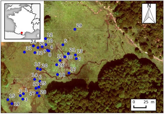
Figure 1.
Location of the in situ spectroradiometer measurements—True color composite made from hyperspectral (HySpex) aerial imageries acquired on the 09/12/2014 (R = 639.98 , G = 549.06 , B = 461.79 ).
2.2. Field Data Collection
In this study, thirteen vegetation units with ecological values and potentials (i.e., biodiversity) have been identified in the Bernadouze peatbog. These units are named hereafter “vegetation types” according to the dominant land cover type or to the potential development of interesting plant species which may have ecological values (Table 1). For each type, several locations have been surveyed to characterize their plant species composition (Table A1).

Table 1.
Species names, number of measurements, number of locations and total number of spectra collected.
For all these 32 sample locations (Figure 1), radiances are measured at three different dates over 9 days in September 2014 (4 September 2014, 5 September 2014, 12 September 2014) under sunny and cloudless conditions between 10:00 a.m. and 1:00 p.m. and Sun’s azimuth angle ranging from 106° and 160°. Data have been collected using an Analytical Spectral Device (ASD) spectroradiometer which ranges on the reflective domain (350–2500 ) with a 3–12 spectral resolution depending on the spectral domain. Its spectral specifications are summarized in Table 2.
Table 2.
Analytical Spectral Device (ASD) FieldSpec Pro specifications.
To measure the reflectance of a sample plot the reflectance of a white reference is required. This latter was obtained with a Spectralon (Labsphere, North Sutton, NH, USA) panel. Finally, after dark current correction, is given by:
where is the measured radiance from the sample plot and is the measured radiance from the white reference.
The sensor was positioned approximatively 1 over the target with a 10° field of view. Consequently the ground spatial resolution is 0.18 . The ASD was configured to collect 20 samples and automatically average in order to provide a single mean spectral measurement. Then a total of 7 to 53 field spectroradiometer measurements, i.e., spectral signatures, depending on vegetation type was taken.
2.3. Data Preprocessing
Some spectral bands (1350 to 1450 , 1810 to 1940 and 2400 to 2500 ) have been removed due to a small signal-to-noise ratio resulting from strong atmospheric absorption mainly due to the presence of water vapour. More precisely, if the atmospheric transmittance value of the U.S. Standard profile was lower than 0.8 for a given wavelength, this wavelength was not taken into account in the analyse. Thus, each measured spectrum has been smoothed using a Savitzky-Golay filter [] for reducing the noise. Figure 2 graphs the mean spectral reflectance of each vegetation type and the atmospheric transmittance. For the sake of clarity, the standard deviation of each vegetation type is not printed on Figure 2 but can be seen in Appendix B.
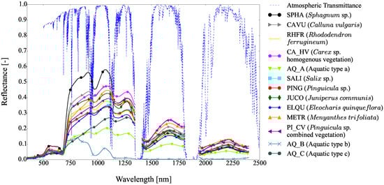
Figure 2.
Mean spectral reflectances of the 13 vegetation types and the U.S. Standard atmospheric transmittance.
3. Method Description
The flowchart to evaluate the potential of hyperspectral data to discriminate between and classify wetland vegetation types is given in Figure 3. More precisely, three classes of methods have been investigated and compared:
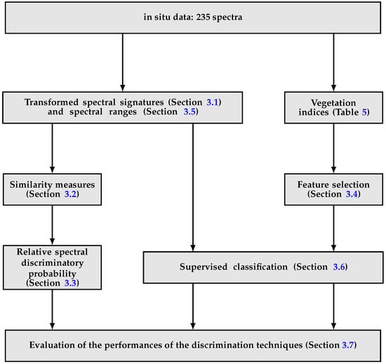
Figure 3.
Flowchart showing the different methods used to classify the vegetation types.
- similarity measures calculated on spectral reflectance,
- supervised classification based on “local” information (spectral vegetation indices),
- supervised classification based on “global” information (spectral ranges).
Indeed, spectral matching can be used to discriminate between different vegetation types, because it is assumed that the spectral signatures of a given vegetation type must have similarities. To catch those similarities, several mathematical transformations—enhancing absorption features are applied on spectral signatures—(Section 3.1) and several similarity criteria—related to distances or spectral shapes or probabilistic behaviour—(Section 3.2) are investigated. Furthermore those similarity measures are applied on several spectral ranges which characterize specific biophysical properties (Section 3.5) and compared to a reference spectral database using relative spectral discriminatory probability (Section 3.3).
On the other hand as it may be difficult to have a spectral reference database, different supervised classifiers are used (Section 3.6). Besides, we assume that specific biophysical properties/components may help discriminating vegetation types. Biophysical components can be used in a local way considering spectral vegetation indices (Section 3.4.3) or in a global way considering spectral ranges and transformed spectral signatures as explained above.
To evaluate performance of similarity measures and supervised classification, the overall accuracy and F1-score are used (Section 3.7).
3.1. Transformed Spectral Signatures
As vegetation types are composed by a mix of various plant species that can be found in various vegetation types, different transformations are used (Table 3). Brightness-normalized spectral signature and second derivative are relatively insensible to variations in illumination intensity causes by changes in sun angle [,]. Other transformations (first derivative, second derivative, log transformation, Continuum Removal, Continuum Removed Derivative Reflectance (CRDR)) are linked to absorption features that may differ from one vegetation type to another, depending on the floristic composition.
Table 3.
Transformed spectral signatures.
3.2. Similarity Measures
Let be a spectral signature, its reflectance at wavelength and its spectral range. Several criteria have been used (Table 4). Some criteria characterize the difference between reflectance levels (like the distances) and other ones are related to the difference of the spectral shape (e.g., SAM) and other ones are related to probabilistic behaviour (e.g., SID, ...). Table 4 inventories main similarity measurement techniques described in the literature.
Table 4.
Similarity measures.
3.3. Relative Spectral Discriminatory Probability
To determine if a spectral signature belongs to a class, the method proposed by [] is used. Let J spectral signatures in an existing spectral reference database and be a target signature to be identified using . Let be a given hyperspectral measure, the spectral discriminatory probabilities of all in with respect to as is defined as follows:
where is a normalization constant determined by and . The resulting probability vector is defined as
Using Equation (3), the target signature can be identified by selecting the one with the smallest spectral discriminatory probability because and the selected one have the minimum spectral discrimination.
Spectral Reference Database
To build the spectral reference database, spectra of mean reflectance, spectra of median reflectance and median spectra are used. Spectra of mean reflectance is defined as the mean of reflectances for each wavelength :
where N is the number of spectra for a plant species. Similarly, spectra of median reflectance is defined as the median of reflectances for each wavelength . Median spectra is defined as the “closest” spectrum of the median reflectance considering a vegetation type. In other words, giving a spectrum of median reflectance, the spectrum that minimize the Minkowski distance between them is considered as the median spectrum (Figure 4 shows differences between the median reflectances spectrum which is an theoretic spectral signature and the different median spectra which were investigated). As distances are not equivalent considering high-dimensional data, three Minkowski distances are investigated for this study: the Euclidean distance, the Canberra distance and the City Block or Manhattan distance (which are reminded in Section 3.1).
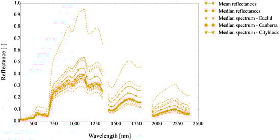
Figure 4.
Median spectra, spectrum of mean reflectances, spectrum of median reflectances of Eleocharis quinqueflora (ELQU).
3.4. Feature Selection of Spectral Indices
3.4.1. Spectral Index Description
Spectral indices are combinations of surface reflectance (or the derivated reflectance) at two or more wavelengths or narrow spectral bands. Lots of spectral indices can be found in literature (Table 5) to characterize some biochemical components of plant species such as chlorophyll, nitrogen, lignin, cellulose, water. Although these indices have never been selected in the literature to characterize wetlands plant species, we assume that some of them can still be useful to classify them.
Table 5.
Spectral vegetation indices.
3.4.2. Classical Feature Selection Method—The Kruskal-Wallis H-Test
As some spectra per vegetation types were quite small (8 spectra for Pinguicula sp. (PING), 7 spectra for Aquatic type b (AQ_B)), usual ANOVA [] test or Mann-Whitney U-test [] can not be used. That is the reason why Kruskal-Wallis H-test [], a non-parametric test is proposed. Moreover this test is adapted to not independent data and not normally distributed data. The H-test is used to test the hypothesis that there was no significant difference between the median spectral index value between pairs of plant species.
The null hypothesis for vegetation types and spectral vegetation indices per reflectance measurements is:
where is the median spectral index value for vegetation type number , and the spectral index. The maximum frequency for this study is . The hypothesis was therefore tested 78 times for all possible combinations of the 13 plant species at the adjusted Bonferroni significance level of .
3.4.3. Principle of the Applied Feature Selection Method
In order to discriminate between the 78 pairs of vegetation types, the Hellinger distance, which is introduced further, is computed for each vegetation spectral index (Table 5). Then indices are ordered by frequency discrimination. A first subset of indices is composed of ones that can discriminate between pairs of vegetation types and that are not redundant. If there is no discrimination between a pair of vegetation types, the Hellinger distance is computed for a pair of vegetation indices composed of the single most discriminating one and the other ones ordered by frequency distribution amongst previous selected. Then, a second subset of pairs of indices is composed by ordering those pairs of indices by frequency discrimination. To stop the process, a maximum number of subsets is then defined. In our case, the maximum subset consists of not more than three indices. Indeed, the longer the tuple length is, the more difficult it is to explained why such combinations of indices or such biophysical components combination can discriminate between such pairs. Finally, selected vegetation indices come from each subset and single spectral vegetation indices or spectral index combinations are retained.
For a better understanding of the feature selection method, an example is given. We consider four vegetation types named: and 5 spectral vegetation indices named: . We suppose that no single spectral vegetation index can discriminate between neither and nor and nor and . But different single indices can separate from , from and from . This is summarized in the following table:
| ine | ∅ | ||
| - | ∅ | ||
| - | - | ∅ |
We obtain the first subset . To discriminate between and , and , and and , we are looking among the following combinations: because indices are ordered by frequency discrimination: []. We suppose that can discriminate between and , and and but there is still no index that can discriminate between and . For the latter case, possible combinations are looking among . Whatever a combination of spectral vegetation indices can be found to discriminate between those plant species or not, the process will stop in our case.
3.4.4. The Bhattacharyya Coefficient and the Hellinger Distance
For two arbitrary discrete probability distributions and , the amount of overlap between those distributions can be measured using the Bhattacharyya coefficient:
where n is the partition number. To measure the similarity between two statistical distributions in remote sensing the Hellinger distance (also known as the Matusita distance) is commonly used. It is defined as:
The Hellinger distance defined in Equation (8) has upper bound equal to 1, indicating the total separability of the class pairs characterized by their distribution. As a general rule adapted from [],
- if then the classes can be separated,
- if the separation is fairly good,
- if the separation is poor.
3.5. Spectral Ranges
The transformed spectral signatures defined in Section 3.2 and the spectral ranges adapted from [] (Table 6) were investigated:
Table 6.
The spectral reflectances of green vegetation on the four regions of electromagnetic spectrum from [].
- visible: 350 –750 ,
- near infrared: 750 –1350 ,
- shortwave infrared a: 1410 –1810 ,
- shortwave infrared b: 1940 –2400 .
The shortwave infrared domain is split into two parts. The near infrared and the shortwave infrared are not continuous because of atmospheric water absorption.
3.6. Supervised Classification
All the classifications are performed using Python scikit-learn package [].
3.6.1. Random Forest (RF)
RF is an ensemble classifier that uses a set of Classification And Regression Trees (CARTs) to make a prediction []. The trees are created by drawing a subset of training samples through replacement (a bagging approach). In standard classification trees, each node is split using the best split among all variables. In RF, each node is split using the best predictor, among a user-defined number of features (Mtry that is usually set to the square root of the number of input variables []). By growing the forest up to a user-defined number of trees (Ntree that is usually set to 500 but different values such as 100, 1000 or 5000 have been investigated []), the algorithm creates trees that have high variance and low bias. The final classification decision is taken by averaging (using the arithmetic mean) the class assignment probabilities calculated by all produced trees.
For this study, Mtry = 500 and Ntree ∈ [500, 1000, 2000, 5000].
3.6.2. Support Vector Machines (SVM)
SVM is a supervised non-parametric statistical learning technique therefore there is no assumption on the distribution of the data []. The main idea of SVM classification is to construct a hyperplane as a decision surface in a way that the margin of separation between two classes is maximized. To do this, the original feature space is mapped into a space with a higher dimensionality, where classes can be modelled to be linearly separable. This transformation is implicitly performed by applying kernel functions to the original data. The learning of the classifier is performed using a constrained optimization process that is associated with a complex cost function. For problems that involve identification of multiple classes, adjustments are made to the simple SVM binary classifier to operate as a multi-class classifier using methods such as one-against-all, one-against-others.
For this study, two kernels are retained: a linear kernel (SVM linear) and a Gaussian kernel (SVM RBF).
3.6.3. Regularized Logistic Regression (RLR)
RLR is a linear model based on logistic regression with an additional regularization term. This classifier has been successfully used with high dimensional data (gene selection in cancer classification [], feature selection in remote sensing [,,]).
For this study, the -norm and -norm regularization term are investigated.
3.6.4. Partial Least Squares-Discriminant analysis (PLS-DA)
PLS-DA is based upon the classical partial least square regression method for constructing predictive models []. The goal of PLS regression is to provide dimension reduction in an application where the response variable is related to the predictor variables. In the case of PLS-DA, the response variable (i.e., vegetation types) is binary and expresses class membership [,]. This classifier has been successfully used with high dimensional data (gene selection [], tree species discrimination []).
For this study the number of latent variables is fixed to the number of vegetation types-1 []. This method is not applied on spectral vegetation indices selected but on spectral signatures and their transformations on spectral ranges because it is commonly used when the number of features is much bigger than the number of spectra.
3.7. Classification Accuracy Evaluation
To evaluate the classification accuracy of supervised classifiers, a 30 fold cross-validation is used and six training samples size were investigated: 50%, 45%, 40%, 35%, 30% and 25% of all spectra.
To evaluate the classifier precision overall accuracy and F1-score are used. Overall accuracy computes number of correct spectra over all spectra, whereas F1-score is given by:
where PA (Producer’s Accuracy) is the fraction of retrieved classes that are relevant whereas UA (User’s Accuracy) is the fraction of relevant classes that are retrieved.
4. Results and Discussion
4.1. Similarity Measures
Considering all transformed spectral signatures, spectral ranges and similarity measures, only the Canberra distance on [350 –2500 ] gives an overall accuracy higher than 50% whatever the spectral reference database (Table 7). Indeed, the Canberra distance gives the higher overall accuracy because it is sensitive to a small change when both coordinates are closed to zero [,].
Table 7.
Overall accuracy (%) for Canberra distance on [350–2500 ].
Because of the high variability of some vegetation types (Appendix B), spectral reference database built from median spectra, that are real spectra, gave worse results than spectral reference database built from median and mean spectra, that are theoretical spectra not representative of a in situ measured vegetation type (Table 7). There is a need to collect more spectral signatures to build a consistent spectral database.
As spectral signatures can be considered as high dimensional vectors, a specific distance is needed to compare them. It is well known that Euclidean distance is not good when comparing high dimension data []. Table 8 shows that the Canberra distance always outperforms other distances, including SAM, which is commonly used in remote sensing, when considering the whole spectral range (1823 wavelengths).
Table 8.
Overall accuracy (%) for different distances on [350–2500 ] considering Median reflectances as spectral reference database.
Using the Canberra distance, best results (overall accuracy higher than 60%) are given with the second derivative, first derivative and CRDR (Table 7), that are closely related to absorption features rather than reflectance magnitude []. Indeed, it is possible to discriminate between vegetation types thanks to their biophysical components which will be discussed in details in Section 4.2.1. Furthermore, Table 9 shows that the whole spectral range gives the best results. Although spectral ranges are related to specific biophysical components (Table 6), the whole spectral range is needed to discriminate between the 13 vegetation types because some of them are sharing same plant species (Table A1) and the spectral signatures are mixed. Worse results are obtained in [1940–2400 ] whatever the transformed spectral signature. Table 9 show that worse results are obtained by the spectral signature whatever the spectral range. Indeed those transformations are related to absorption features as explained above, which confirms that transformed spectral signatures are more suitable to discriminate between vegetation types than spectral signatures.
Table 9.
Overall classification accuracy (%) for different spectral ranges considering Median reflectances as spectral reference database and Canberra distance.
Considering classification accuracy for each vegetation type, Table 10 shows that best F1-score is obtained by Sphagnum sp. (SPHA) (≃98%), Juniperus communis (JUCO) (≃97%), AQ_B (≃93%) and Salix sp. (SALI) (≃92%). Except for JUCO, all of these vegetation types are well classified and their user’s accuracy is higher than 85%. Indeed these vegetation types are less mixed than others: Table A1 shows that SPHA is mainly dominated by different kinds of sphagnum; AQ_B is dominated by Utricularia sp; JUCO is dominated by Juniperus communis and SALI is dominated by Salix. Only three other vegetation types have user’s accuracy equal to 100%: Rhododendron ferrugineum (RHFR), Calluna vulgaris (CAVU) and Aquatic type a (AQ_A). However, only around 57% of spectral signatures are well identified for CAVU and AQ_A. This can be explained by the high variability of these sample plots. Contrary to SPHA, JUCO, AQ_B and SALI, there is not a single dominated plant species neither for CAVU nor for AQ_A (Table A1). Worse F1-score is obtained by Pinguicula sp. (PING) (≃54%) which is not dominated by only one plant species: this vegetation type is mainly dominated by Eleocharis quinqueflora (ELQU) (40%), bare ground (15%), Molinia caerulea ssp caerulae (10%) and Tomenthypnum nitens (10%). It can explain the difficulty to identify this vegetation type in particular rather than the low number of spectra: PING has eight spectra whereas AQ_B has seven spectra.
Table 10.
Confusion matrix of the classification based on Second derivative, Canberra Distance on [350–2500 ] with Median reflectance as reference spectral database. The producer’s and user’s accuracies, the overall accuracy and the F1-score are also shown.
4.2. Supervised Classification Based on Feature Selection of Spectral Vegetation Indices
4.2.1. Feature Selection
The Kruskal-Wallis method (Section 3.4.2, p. 13) does not show any significant index (frequency discrimination ) that allow discrimination between vegetation types (Figure 5, only the first 69 indices are drawn). The best vegetation index (NDWI [860, 2130]) only allows us to discriminate between 49 pairs of vegetation types, that may be explained by the plant species mixing within several vegetation types. The proposed method reduced the number of selected indices from 129 to 26 (Table 11). More precisely, on the first step of the method, only 17 single indices amongst 26 are needed to discriminate between 59 pairs of vegetation types amongst 78. On the second step, these single indices must be completed by 7 additional spectral vegetation indices to discriminate between 17 more pairs of vegetation types (Table 12; ∅ means either a pair of vegetation type can not be discriminated thanks to a pair of spectral vegetation indices built from single ones selected on the first step, either more than two vegetation indices are needed to discriminate between a pair of vegetation types). On the last step, a single index is added to discriminate between two vegetation types whereas a combination of previous selected indices allows us to discriminate between another pair of vegetation type (Table 11). Finally several different—single or pair or triplet—vegetation indices allow us to discriminate between pairs of vegetation types. However, none single spectral index allows us to discriminate between all pairs of vegetation types nor the majority: e.g., the most discriminating single spectral index, the Water Index (WI), only discriminates between around 42% pairs of vegetation types (Table 11).
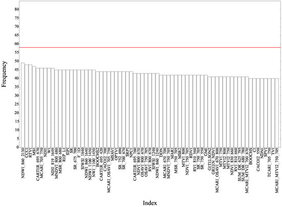
Figure 5.
Frequency distribution of the Kruskal-Wallis test for the 129 spectral indices for paired species across the 13 vegetation types. The horizontal red line stands for 75% of all 78 possible combinations of the 13 vegetation types.
Table 11.
Single selected indices from the Hellinger distance and their occurrences.
Table 12.
Single spectral index or pairs of spectral indices retained to discriminate between vegetation types pairs.
Table 13 shows that one single biophysical component can discriminate between most of the vegetation types except for Carex sp. homogeneous vegetation (CA_HV). More precisely, three kinds of vegetation types (Sphagnum sp. (SPHA), Aquatic type b (AQ_B) and Aquatic type c (AQ_C)) are separated thanks to a single biophysical component. However, some biophysical components are more discriminant than others according to vegetation types: e.g., the chlorophyll is more discriminant than the water content for AQ_C whereas the water content is the only discriminant biophysical component for AQ_B; the water content, the chlorophyll and water, cellulose, starch, lignin (w., c., s., l.) equally discriminate between SPHA and all other vegetation types.
Table 13.
Single main discriminating biophysical components for each vegetation type and their occurrences (%).
Only two indices related to water content are needed to separate AQ_B from all other vegetation types: WI and NDWI[860,1240] (Table 13) because AQ_B vegetation type is mainly composed of Utricularia sp. and water (Table A1). The AQ_B spectral signatures are lower than the spectral reflectance values of the other vegetation types and the water absorption band at 900 and 970 are highlighted (Figure 6).
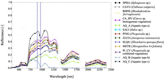
Figure 6.
Mean spectral reflectance of the 13 vegetation types. Dashed lines represent the wavelengths used by Water Index (WI).
The chlorophyll is the main biophysical component (86.33%) able to discriminate between AQ_C and all other vegetation types, except with Aquatic type a (AQ_A) and AQ_B differentiated by considering additional water indices (MSI and NDWI [860,1240]). Indeed, dry matter can be seen on spectral signatures (Figure 7): AQ_B has the lowest slope on the spectral range [705–730 ] whereas other vegetation types (except AQ_A and AQ_B) have higher values because they still contain chlorophyll. However, as AQ_B and AQ_C have low values of Boochs2 index, it is possible to discriminate between them thanks to a water index (right side of Figure 8 shows that those vegetation types can be clearly separated; indeed, those vegetation types have different shapes and values that characterize each type).
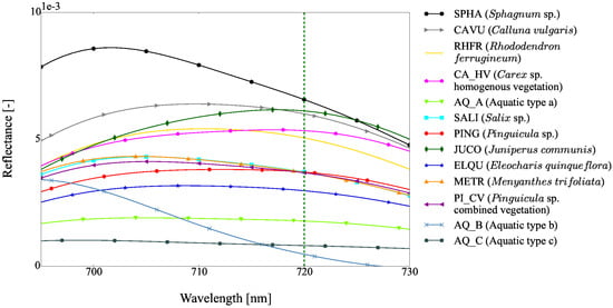
Figure 7.
Mean first derivative spectral signatures of the 13 vegetation types on [695–730 ]. The green dashed line represents the wavelength used by the Boochs2 index.
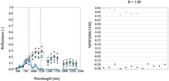
Figure 8.
(Left) spectral signatures of AQ_B (blue) and AQ_C (dark slate gray). Red dashed lines are the wavelengths used by the Normalized Difference Water Index (NDWI) [860,1240] index; (Right) NDWI [860,1240] values for each vegetation type, H is the Hellinger distance.
In some case, there is no single biophysical component allowing us to discriminate between vegetation types: e.g., both water content (33.33%), chlorophyll (33.33%) and w., c., s., l. (33.33%) are needed to distinguish SPHA from all other vegetation types (Table 13). More precisely, biophysical components related to water (WI, MSI) are discriminating SPHA from CA_HV, Pinguicula sp. (PING), Pinguicula sp. combined vegetation (PI_CV) and AQ_B ; biophysical components related to chlorophyll (CCCI, OSAVI [800,670]) are differentiating SPHA from AQ_A, AQ_C, Eleocharis quinqueflora (ELQU) and Menyanthes trifoliata (METR) ; biophysical components related to w., c., s., l. (F_WP) are separating SPHA from Calluna vulgaris (CAVU), Rhododendron ferrugineum (RHFR), Salix sp. (SALI) and Juniperus communis (JUCO) (Table 13). Unlike an index related to water content (Figure 9), an index related to the chlorophyll will discriminate between SPHA and AQ_A. Indeed, the right side of Figure 9 shows that some AQ_A plant species can not be distinguished from SPHA because it is a dry moss and the left side of Figure 9 shows that SPHA and non discerned AQ_A have the same spectral signature shape. The right side of Figure 10 shows that these two vegetation species can clearly be separated despite the class variability of AQ_A. A complex biophysical component such as F_WP will differentiate SPHA from CAVU (left side of Figure 11) shows that different spectral shapes between those vegetation types can be exploited on the [1220–1280 ] domain. The right side of Figure 10 shows that the wavelengths corresponding to the maximum of the first derivatives can clearly discern these two vegetation types even if these vegetation types can be mixed.
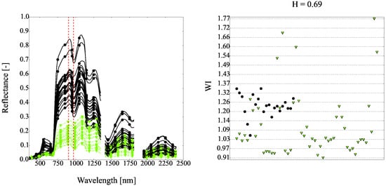
Figure 9.
(Left) spectral signatures of Sphagnum sp. (SPHA)! (black) and AQ_A (green). Red dashed lines are WI wavelengths; (Right) WI values for each vegetation type, H is the Hellinger distance.
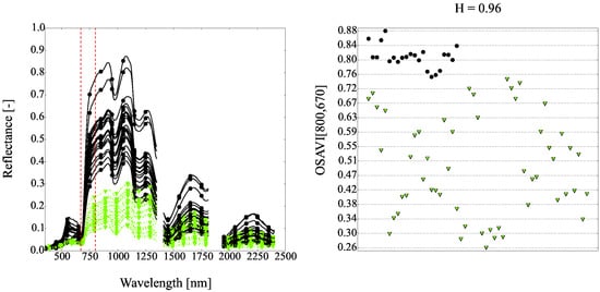
Figure 10.
(Left) spectral signatures of SPHA (black) and AQ_A (green). Red dashed lines are Optimised Soil-Adjust Vegetation Index (OSAVI) [800,670] wavelengths; (Right) OSAVI [800,670] values for each vegetation type, H is the Hellinger distance.
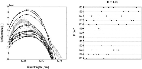
Figure 11.
(Left) spectral signatures of SPHA (black) and Calluna vulgaris (CAVU) (gray); (Right) F_WP values for each vegetation type, H is the Hellinger distance.
In most cases, a single biophysical component is sufficient to class a vegetation type from the others (except for CA_HV), but a pair of biophysical components is needed to discriminate more specifically between some vegetation types (Table 12), apart from some particular cases where a pair of biophysical components is needed CA_HV (Figure 12). Indeed, CAVU and SALI are differentiated with the stress index (CARTER [695, 420]) and the water index (NDII).
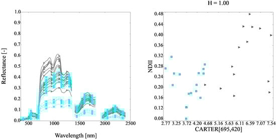
Figure 12.
(Left) spectral signatures of CAVU (gray) and Salix sp. (SALI) (cyan); (Right) map of CARTER[695,420] and Normalized Difference Infrared Index (NDII) values for each vegetation type, H is the Hellinger distance.
Among the 78 combinations of pair of vegetation types, only two require three indices to be separated: CA_HV vs. PING and AQ_A vs. METR. Indeed, because of its within class variability (Table A1), only 33.33% of a single biophysical component can discriminate between CA_HV and all other vegetation types (Table 13). Besides, as mentioned in Section 4.1, none of the main plant species of PING represents more than 50% of this vegetation type. The advent of a third index only improves significantly their discrimination (Figure 13).
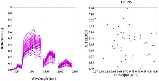
Figure 13.
(Left) spectral signatures of CA_HV (pink) and PI_CV (magenta); (Right) map of Optimised Soil-Adjust Vegetation Index (OSAVI) [800,670] and GITELSON values for each vegetation type, H is the Hellinger distance value.
4.2.2. Supervised Classification
The 26 indices selected with the Hellinger distance enables overall classification accuracy scores ranging from 72.90% to 85.20% depending on the training size, whereas when considering all indices overall accuracy, scores range from 66.70% to 82.80% (Table 14). Moreover, these selected indices are robust because no significant difference between classifiers score (except for RF) regardless of the training size is noted (Figure 14). As expected, the worst results are given by the Kruskal-Wallis method (to compare performance of the two features selection methods, 26 first indices given by Kruskal-Wallis method have been selected).
Table 14.
Vegetation types identification (overall accuracy (±standard deviation) in %) with indices.
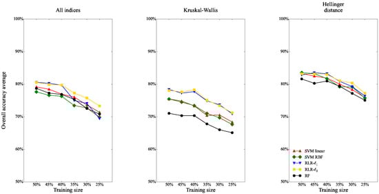
Figure 14.
Vegetation types identification accuracies (overall accuracy) with indices.
RLR gives better results than SVM and RF (Table 14, Figure 14) except when the size of the training set equals 50% for the Hellinger distance. That may be explained by the possible confusion between some vegetation types due to their plant species composition. Indeed, SVM aims to find the best hyperplane that can separate data, whereas RLR aims to find a probability (according to a logistic function) to separate them.
Considering RLR- some vegetation types are not easily discriminated whatever the indices. Table 15 and Table 16 show that PING has the lowest F1-score (20.99% and 33.13% respectively) which can be explained by the mixed composition of this habitat (Appendix B) and not the low number of spectra. Indeed, AQ_B has about the same number of spectra: 7 spectra whereas 8 spectral measurements have been collected for PING. Yet it has a F1-score = 91.95% considering all indices and F1-score = 91.66% considering indices selected by the Hellinger distance that can be explained by its composition dominated by Utricularia sp.
Table 15.
Confusion matrix of the classification based on Regularized Logistic Regression (RLR)- with all indices and training size = 25%. The producer’s and user’s accuracies and the overall accuracy average (OAA) are also shown.
Table 16.
Confusion matrix of the classification based on RLR- with indices selected by the Hellinger distance and training size = 25%. The producer’s and user’s accuracies and the overall accuracy average (OAA) are also shown.
Focusing on shrubs, JUCO has the best performances (F1-score = 94.83%) whereas SALI and RHFR are often confounded. Table 16 shows that on average 2.53 spectra of RHFR (≃20.02%) are classified as SALI and on average 2.30 spectra of SALI (≃19.15%) are classified as RHFR. Indeed, as JUCO has a higher foliage density, the overall spatial signature is less sensitive to the ground influence and as a result JUCO spectral reflectance is close to a pure endmember (Appendix B). In the latter case, the spectral measurements are composed of soil and more affected by mixed signatures. Another pair of vegetation types is hardly discriminated: PI_CV and CA_HV. Table 16 shows that on average 4.93 spectra of CA_HV (≃25%) are classified as PI_CV which may be explained by the plant species they have in common: Carex (50–100% depending on the location) and Molinia caerulea ssp. caerulae (40–70%) (Appendix B).
4.3. Supervised Classification According to the Spectral Ranges
Only the best results are presented, obtained with the four spectral ranges ([350–750 ], [750–1350 ], [350–1350 ], [350–2500 ]) and the spectral signature as reference and the three transformed spectral signatures (second derivative, first derivative, Continuum Removed Derivative Reflectance).
Table 17, Table 18, Table 19 and Table 20 show the best results obtained with RLR- on [350–1350 ] whatever the transformed spectral signatures.
Table 17.
Vegetation types identification accuracies (overall accuracy (±standard deviation) in %) on [350–750 ].
Table 18.
Vegetation types identification accuracies (overall accuracy (±standard deviation) in %) on [750–1350 ].
Table 19.
Vegetation types identification accuracies (overall accuracy (±standard deviation) in %) in [350–1350 ].
Table 20.
Vegetation types identification accuracies (overall accuracy (±standard deviation) in %) on [350–2500 ].
Considering wavelengths used by selected indices (Section 4.2.1), most of them use spectral bands located on [350–1350 ] either: 50% are located in visible range and 32.35% in near-infrared range. Indeed, in this spectral range all the biophysical components discriminating the peatland vegetation types can be taken into account. That is confirmed by Figure 15 which shows that the best results are given by [350–1350 ] considering the training size = 25% regardless the transformed spectral signatures and the the classifier, except for RF applied on the spectral signature. In this case, considering the whole spectral range improves the result by 1% compared with [350–1350 ].
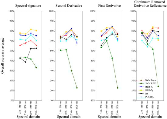
Figure 15.
Vegetation type identification accuracies with the training size = 25%.
Considering RLR- in [350–1350 ], Table 21 shows that the best overall accuracies are given by first derivative, second derivative and CRDR. First and second derivatives overall accuracies are very close (difference lower than 1%). However, those transformations are sensitive to noise. However, CRDR delivered better results than spectral signatures and similar performances to the first and second derivatives (difference is lower than 4%). As mentioned in Section 4.1, those transformations are closely related to absorption features rather than reflectance magnitude [], and are helpful to discriminate between peatland vegetation types which are clearly characterized by different biophysical components as mentioned in Section 4.2.1.
Table 21.
Vegetation types identification accuracies (overall accuracy (±standard deviation) in %) on [350–1350 ] for RLR-.
Considering RLR, regularization, which controls the selection or the removal of variables, always underperforms -regularization, which handles collinear variables []. Because of mixed plant species, it is difficult to remove variables that are not involved in the classification of all the vegetation types. Although SVM and RF are popular classifiers in remote sensing community, they are outclassed by RLR in [350 –1350 ] which is the spectral range where results are the best (Figure 16). Results given by SVM RBF are lower than those obtained with RLR and can be explained by the difficulty to find adapted parameters considering this high dimensionality problem. However, it is interesting to note that results from SVM linear are close to RLR ones considering first derivative, second derivative and CRDR. Further investigations should be conducted to better understand the link between those classifiers and improve the choice of the parameters. Figure 16 shows that PLS-DA is the least sensitive classifier to training size regardless transformed spectral signatures in [350–1350 ].
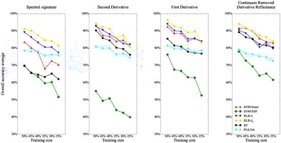
Figure 16.
Vegetation type identification accuracies on [350–1350 ].
Table 22 shows that Pinguicula sp. (PING) has the lowest F1-score (66.67% and 56.00% respectively) as well as for the spectral vegetation indices (Section 4.2.2). Besides, this vegetation type can hardly be discriminated from the other ones (Producer’s accuracy (PA) = 53.33%) and some Pinguicula sp. combined vegetation (PI_CV) spectra are classified as PING). However, it should be kept in mind that PING has a small number of spectra. Considering Aquatic type b (AQ_B) which has about the same number of spectra (7 spectra against 8 for PING), User’s Accuracy (UA) = 60.98% and some Aquatic type a (AQ_A) spectra are predicted as AQ_B ones. These poor UA results compared to one obtained by spectral vegetation indices can not be explained by the spectral domain. Indeed, the best spectra vegetation index (NDWI[860,1240]) that discriminate between AQ_A and AQ_B has both wavelengths in [350–1350 ]. However, this result may be qualified by PA. Indeed, on [350–1350 ] domain, UA = 100.00% whereas UA = 84.60% for spectral vegetation indices. Nevertheless, using a continuous spectral domain can lead to worse results for other vegetation types such as Sphagnum sp. (SPHA), Calluna vulgaris (CAVU), AQ_A: F1-score is always better considering the same classifier (RLR-) applied on spectral vegetation indices selected by the Hellinger distance (SPHA: 91.12% vs. 82.80%; CAVU: 77.62% vs. 71.43%; AQ_A: 86.80% vs. 82.81%). Considering SPHA, if PA = 90.59% for spectral vegetation indices or for [350–1350 ], the latter predicts more SPHA than observed (UA = 76.24%) and is more confused with CAVU. This can be explained by plot 7 which is mainly composed of Calluna vulgaris (20%), Carex rostrata (25%), Molinia caerulea ssp. caerulae (20%) and Sphagnum palustre (20%) (Appendix B).
Table 22.
Confusion matrix of the RLR- classification using Continuum Removed Derivative Reflectance (CRDR) on [350–1350 ] (training size = 25%). The producer’s and user’s accuracies, the overall accuracy and the F1-score are also shown.
In our case, reducing feature space by selecting most discriminant wavelengths (using PCA or MNF) has not been implemented, whereas it can be an interesting track to explore to see if it improves results for RLR-. Juniperus communis (JUCO), Eleocharis quinqueflora (ELQU) and Aquatic type c (AQ_C) have about the same F1-score considering spectral vegetation indices or [350–1350 ]: less than 2% difference. However, they have better PA on the continuous spectral range (PA = 100.00% for JUCO; 95.56% for AQ_C) which means that this spectral range contains discriminant wavelengths able to catch characteristics of those vegetation types.
Rhododendron ferrugineum (RHFR), Carex sp. homogeneous vegetation (CA_HV), Salix sp. (SALI) and Menyanthes trifoliata (METR) have better results considering [350–1350 ]. This can be explained by the fact that the spectral vegetation indices used have not been built for that kind of vegetation type. Further investigations can be undertaken to find specific indices that can discriminate between those vegetation types and other ones.
5. Conclusions and Perspectives
This study aimed at inventorying and evaluating the performance of discrimination techniques for peatland habitats based on in situ hyperspectral measurements with a high spectral resolution and high signal-to-noise ratio. To evaluate the potential of hyperspectral data to separate and classify those habitats, three classes of methods were investigated and compared:
- similarity measures calculated on spectral reflectance,
- supervised classification based on “local” information (spectral vegetation indices),
- supervised classification based on “global” information (spectral ranges).
This study demonstrated that is it possible to discriminate between peatland vegetation types by using the Canberra distance on the whole spectral range [350–2500 ]. This distance is sensitive to a small change when both coordinates approach zero which is the case of reflectance especially in the visible ranges and in the SWIR (Figure 2). Further investigations should be conducted to see if combinations of spectral range can improve overall accuracy or if the lack of spectral signatures in the reference database (which is a weakness of this method) may explain why the whole spectral range is needed to compare spectra in that case. Besides, it is of importance to collect more spectral signatures from peatland vegetation types to build a spectral reference database of peatland vegetation types that can catch more spectral variability.
Although there are no spectral vegetation indices built to discriminate between peatland vegetation types, this study showed that some indices could be selected using the Hellinger distance. Although those indices have not been built to discriminate between peatland vegetation types, they were able to classify them because they focus on biochemical properties such as chlorophyll, nitrogen, water stress, etc. Further investigations have to be done to see the impact of spectral bandwidth around the wavelength of selected indices instead of working with one particular wavelength. For instance, there are lots of indices that catch the same biochemical property but wavelengths of interest change because they focus on specific plant species (e.g., for the chlorophyll, SR [700,670] is built for field corn, whereas SR [675,700] is built for soy beans leaves; contrary to SR [675,700], SR [700,670] has been selected with the Hellinger distance).
Contrary to similarity measures which had the best results considering the whole spectral range, supervised classification on specific spectral range as defined by [] achieved the best overall accuracy considering [350–1350 ] domain. This is in agreement with the spectral vegetation indices: only 4 indices (NDWI [860, 1240], NDWI [860, 2130], NDWI [1110, 1450], MSI) over the 26 selected have a discriminant wavelength which is not in this spectral range. More precisely, the discriminant wavelength is located in the SWIR and all concerned vegetation indices are linked to the water status. Further investigations should be conducted on the extraction or the reduction of features of this spectral range to understand why this domain sometimes gave worse results than spectral vegetation indices depending on the vegetation type.
Among the three methods, the best results are obtained considering a specific spectral domain [350–1350 ] with RLR regardless of the transformed spectral signatures and the size of the training size (overall accuracy ranges from 81.47% to 96.36%). However, it should be of interest to apply feature reduction methods usually applied on remote sensing (such as PCA or MNF) to see it results are improved or specific spectral wavelength can be selected.
To our knowledge, although not popular in remote sensing for classifying (but already used for feature selection), the RLR classifier achieves the best overall classification accuracy when applied to the spectral vegetation indices selected by the Hellinger distance (77.21%) on the [350–1350 ] domain (83.84%) considering training size = 25%.
Furthermore, this study showed that CRDR gave encouraging results event if it is slightly below those obtained by the first derivative and the second derivative considering RLR classifier.
Considering the habitats, some vegetation types were more easily separated. For instance, JUCO had the best F1-score with the spectral vegetation indices selected by the Hellinger distance (94.83%) or on the [350–1350 ] (95.24%) with RLR and the training size = 25%. In some cases, this specific spectral domain gave better results (F1-score = 92.21% whereas with spectral vegetation indices F1-score = 64.72% for SALI) while in other case, the spectral vegetation indices gave better results (F1-score = 91.12% whereas F1-score = 82.80% for SPHA). As mentioned earlier, reducing feature space needs to be investigated to see if a particular feature space exists that can discriminate between and classify all vegetation types or if we need to consider either spectral vegetation indices or a specific spectral domain depending on the vegetation type to classify.
Although all the results strongly depended on the current dataset, this study illustrated promising methods for classifying peatland vegetation types using in situ hyperspectral measurements. The next step concerns the application or adaptation of those methods to airborne hyperspectral imageries with high spatial resolution acquired on September 2014 (simultaneously with in situ measurements). With the objective of evaluating the benefits of airborne or spaceborne sensors with a lower spectral resolution a lower signal-to-noise ratio, these conclusions may change. For that purpose, some indices (involving wavelengths lower than 480 ) will not be used because of the camera spectral range sensitivity and some transformed spectral signatures such as second derivative will also not be used because of signal-to-noise ratio. Similarly, the first derivative transformation is very sensitive to the noise coming from the instrument but also from the atmosphere correction and this can degrade its performance.
Additional imageries acquired in October 2012 and July 2013 would allow us to test these methods with spectral signatures extracted from the ancillary dataset. Multi-temporal analysis could also be conducted to discriminate between vegetation types thanks to the phenological changes. This step would be of interest to evaluate the robustness of spectral measurements, spectral vegetation indices and classifiers selected previously from in situ hyperspectral measurements to airborne data.
Acknowledgments
The authors would like to thank Rosa Oltra-Carrió and Olivier Vaudelin for their help with field measurements and acknowledge the LabEx DRIIHM and the Observatoire Hommes-Milieux (OHM-CNRS) Haut-Vicdessos for funding and supporting the study.
Author Contributions
Thierry Erudel conducted the analyses and wrote most of the manuscript. Florence Mazier helped with floristic survey data. Thomas Houet, Sophie Fabre and Xavier Briottet helped with the field measurements and contributed as supervisors. All authors contributed to the preparation of the manuscript.
Conflicts of Interest
The authors declare no conflict of interests.
Appendix A. Composition of Vegetation Types
Table A1.
Presence (+) and actual cover percentage of plant species collected on Bernadouze peatbog (Ariège, France) by Florence Mazier & Nicolas de Munik (2014/09/04 & 2014/09/11).
Table A1.
Presence (+) and actual cover percentage of plant species collected on Bernadouze peatbog (Ariège, France) by Florence Mazier & Nicolas de Munik (2014/09/04 & 2014/09/11).
| Plant Species/Plots | 1 | 2 | 3 | 4 | 5 | 6 | 7 | 8 | 9 | 10 | 11 | 12 | 13 | 14 | 15 | 16 |
| Code | SPHA | SPHA | SPHA | SPHA | SPHA | CAVU | CAVU | ELQU | ELQU | PING | METR | JUCO | JUCO | RHFR | RHFR | SALI |
| Alchemilla glabra | ||||||||||||||||
| Anthoxanthum odoratum | 2 | 2 | 2 | 1 | + | |||||||||||
| Apiaceae | ||||||||||||||||
| Bare ground | 1 | 5 | 4 | 15 | ||||||||||||
| Briza media | 2 | + | ||||||||||||||
| Calluna vulgaris | 2 | 5 | 15 | 70 | 25 | + | ||||||||||
| Caltha palustris | 5 | |||||||||||||||
| Campyllium stellatum | 35 | |||||||||||||||
| Cardamine pratensis | + | + | ||||||||||||||
| Carex demissa | ||||||||||||||||
| Carex echinata | 5 | 2 | 2 | + | 2 | + | + | 5 | ||||||||
| Carex flava | + | + | ||||||||||||||
| Carex nigra | 5 | 2 | 2 | 2 | 10 | 5 | ||||||||||
| Carex panicea | + | + | + | 5 | 1 | |||||||||||
| Carex paniculata | ||||||||||||||||
| Carex rostrata | 5 | |||||||||||||||
| Carex sp. | 2 | 25 | ||||||||||||||
| Circaea lutetiana | 4 | |||||||||||||||
| Cirsium palustre | 2 | |||||||||||||||
| Dactylorhiza masculata | 2 | + | + | |||||||||||||
| Drepanocladus revolvens | 30 | |||||||||||||||
| Drosera rotundifolia | + | + | 1 | + | ||||||||||||
| Dryopteraceae | + | |||||||||||||||
| Eleocharis quinqueflora | 60 | 40 | 40 | |||||||||||||
| Epikeros pyrenaeus | + | + | + | |||||||||||||
| Equisetum sp. | 1 | + | + | + | 5 | |||||||||||
| Eriophorum angustifolium | 5 | 10 | ||||||||||||||
| Festuca rubra | 3 | |||||||||||||||
| Galium palustre | ||||||||||||||||
| Galium saxatile | 1 | 2 | ||||||||||||||
| Gentiana ciliata | + | |||||||||||||||
| Hylocomium brevirostre | ||||||||||||||||
| Hypnum cupressiforme | 2 | |||||||||||||||
| Juncus alpinus | + | |||||||||||||||
| Juncus bulbosus | ||||||||||||||||
| Juncus sp. | ||||||||||||||||
| Juniperus communis | 5 | 95 | 80 | |||||||||||||
| Lathyrus montanus | 5 | + | ||||||||||||||
| Leotodon hispidus | ||||||||||||||||
| Lotus sp. | + | 2 | ||||||||||||||
| Luzula sp. | ||||||||||||||||
| Lychnis floscuculi | 4 | |||||||||||||||
| Mentha arvensis | ||||||||||||||||
| Menyanthes trifoliata | 10 | |||||||||||||||
| Moliniacaerulea ssp. caerulae | 15 | 25 | 30 | 15 | 20 | 10 | 20 | 15 | 5 | 10 | 30 | 5 | ||||
| Narthecium ossifragum | 2 | |||||||||||||||
| Parnassia palustris | 1 | 4 | + | 1 | 2 | 3 | ||||||||||
| Pedicularis sylvatica | 1 | + | ||||||||||||||
| Pilosella lactucella | + | 1 | ||||||||||||||
| Pinguicula sp. | 1 | |||||||||||||||
| Pinguicula vulgaris | + | 5 | ||||||||||||||
| Plagiomnium elatum | ||||||||||||||||
| Plantago lanceolata | ||||||||||||||||
| Polytrichum sp. | 2 | |||||||||||||||
| Potentilla erecta | 5 | 5 | 5 | 5 | 10 | 5 | 6 | 5 | 2 | + | ||||||
| Potentilla sp. | ||||||||||||||||
| Prunella vulgaris | + | 2 | ||||||||||||||
| Ranunculus acris | + | |||||||||||||||
| Rhododendron ferrugineum | ||||||||||||||||
| Salix atrocinerea | ||||||||||||||||
| Scorpidium sp. | ||||||||||||||||
| Selaginella selaginoides | + | 1 | ||||||||||||||
| Sphagnum capillifolium | 10 | 5 | 5 | 70 | 25 | |||||||||||
| Sphagnum palustre | 90 | 75 | 65 | 10 | 80 | 20 | 20 | 8 | ||||||||
| Sphagum papillosum | 15 | 25 | ||||||||||||||
| Sphagunm cuspidatum | ||||||||||||||||
| Succisa pratensis | + | |||||||||||||||
| Tofieldia calyculata | + | |||||||||||||||
| Tomenthypnum nitens | 3 | 30 | 10 | |||||||||||||
| Trichophorum cespitosum | + | |||||||||||||||
| Trifolium arvense | ||||||||||||||||
| Trifolium pratense | 1 | 1 | ||||||||||||||
| Utricularia sp. | ||||||||||||||||
| Vaccinium myrtillus | + | 3 | ||||||||||||||
| Vicia sepium | ||||||||||||||||
| Viola palustris | 2 | |||||||||||||||
| Viola sp. | + | 5 | ||||||||||||||
| Water | ||||||||||||||||
| Plant Species/Plots | 17 | 18 | 19 | 20 | 21 | 22 | 23 | 24 | 25 | 26 | 27 | 28 | 29 | 30 | 31 | |
| Code | SALI | SALI | AQ_A | AQ_A | AQ_A | AQ_A | AQ_A | AQ_A | AQ_B | AQ_C | CA_HV | CA_HV | CA_HV | CA_HV | PI_CV | |
| Alchemilla glabra | 2 | + | 3 | |||||||||||||
| Anthoxanthum odoratum | ||||||||||||||||
| Apiaceae | + | |||||||||||||||
| Bare ground | 40 | |||||||||||||||
| Briza media | 5 | 5 | ||||||||||||||
| Calluna vulgaris | ||||||||||||||||
| Caltha palustris | 10 | 2 | 1 | |||||||||||||
| Campyllium stellatum | ||||||||||||||||
| Cardamine pratensis | ||||||||||||||||
| Carex demissa | ||||||||||||||||
| Carex echinata | 1 | 2 | 2 | |||||||||||||
| Carex flava | ||||||||||||||||
| Carex nigra | ||||||||||||||||
| Carex panicea | ||||||||||||||||
| Carex paniculata | 50 | 100 | ||||||||||||||
| Carex rostrata | 35 | 70 | 40 | 10 | ||||||||||||
| Carex sp. | 2 | 60 | 50 | |||||||||||||
| Circaea lutetiana | ||||||||||||||||
| Cirsium palustre | 5 | |||||||||||||||
| Dactylorhiza masculata | + | |||||||||||||||
| Drepanocladus revolvens | + | |||||||||||||||
| Drosera rotundifolia | ||||||||||||||||
| Dryopteraceae | ||||||||||||||||
| Eleocharis quinqueflora | 70 | |||||||||||||||
| Epikeros pyrenaeus | ||||||||||||||||
| Equisetum sp. | 5 | 1 | 30 | + | + | + | + | + | ||||||||
| Eriophorum angustifolium | ||||||||||||||||
| Festuca rubra | 1 | + | 10 | |||||||||||||
| Galium palustre | + | 2 | ||||||||||||||
| Galium saxatile | + | + | 1 | |||||||||||||
| Gentiana ciliata | ||||||||||||||||
| Hylocomium brevirostre | + | |||||||||||||||
| Hypnum cupressiforme | ||||||||||||||||
| Juncus alpinus | ||||||||||||||||
| Juncus bulbosus | 1 | |||||||||||||||
| Juncus sp. | + | |||||||||||||||
| Juniperus communis | ||||||||||||||||
| Lathyrus montanus | + | |||||||||||||||
| Leotodon hispidus | ||||||||||||||||
| Lotus sp. | ||||||||||||||||
| Luzula sp. | + | |||||||||||||||
| Lychnis floscuculi | + | 1 | ||||||||||||||
| Mentha arvensis | + | 2 | ||||||||||||||
| Menyanthes trifoliata | 5 | 10 | 10 | 4 | ||||||||||||
| Moliniacaerulea ssp. caerulae | 5 | 5 | 4 | 60 | 70 | 40 | 50 | |||||||||
| Narthecium ossifragum | + | |||||||||||||||
| Parnassia palustris | + | 2 | 2 | 2 | + | 1 | ||||||||||
| Pedicularis sylvatica | + | |||||||||||||||
| Pilosella lactucella | 1 | |||||||||||||||
| Pinguicula sp. | ||||||||||||||||
| Pinguicula vulgaris | ||||||||||||||||
| Plagiomnium elatum | ||||||||||||||||
| Plantago lanceolata | + | 2 | + | + | ||||||||||||
| Polytrichum sp. | ||||||||||||||||
| Potentilla erecta | 3 | 2 | 1 | 2 | ||||||||||||
| Potentilla sp. | + | |||||||||||||||
| Prunella vulgaris | 4 | 5 | 1 | 1 | ||||||||||||
| Ranunculus acris | 1 | + | 2 | + | ||||||||||||
| Rhododendron ferrugineum | ||||||||||||||||
| Salix atrocinerea | 90 | 100 | ||||||||||||||
| Scorpidium sp. | 4 | 25 | ||||||||||||||
| Selaginella selaginoides | 1 | 1 | ||||||||||||||
| Sphagnum capillifolium | ||||||||||||||||
| Sphagnum palustre | ||||||||||||||||
| Sphagum papillosum | ||||||||||||||||
| Sphagunm cuspidatum | 25 | |||||||||||||||
| Succisa pratensis | 4 | |||||||||||||||
| Tofieldia calyculata | ||||||||||||||||
| Tomenthypnum nitens | 1 | |||||||||||||||
| Trichophorum cespitosum | ||||||||||||||||
| Trifolium arvense | 1 | |||||||||||||||
| Trifolium pratense | 4 | 5 | 2 | 1 | ||||||||||||
| Utricularia sp. | 5 | 80 | ||||||||||||||
| Vaccinium myrtillus | ||||||||||||||||
| Vicia sepium | ||||||||||||||||
| Viola palustris | ||||||||||||||||
| Viola sp. | + | 1 | + | |||||||||||||
| Water | 50 | 25 | 70 | 30 | 60 | 90 | 20 |
Appendix B. Data from Vegetation Types
Appendix B.1. Sphagnum sp. (SPHA)

Figure A1.
Location of the in situ spectroradiometer measurements for the plots of Sphagnum sp. (SPHA).

Figure A2.
Mean reflectance () and standard deviation () of Sphagnum sp. (SPHA).
Table A2.
Pictures, plots, geographic coordinates and number of spectra of Sphagnum sp. (SPHA).
Table A2.
Pictures, plots, geographic coordinates and number of spectra of Sphagnum sp. (SPHA).
| Picture | Plot | Longitude (DD) | Latitude (DD) | Altitude (m) | No. of Spectra |
|---|---|---|---|---|---|
 | 1 | 1.423156 | 42.802105 | 1343.715 | 4 |
 | 2 | 1.423080 | 42.802068 | 1344.046 | 4 |
 | 3 | 1.423143 | 42.802005 | 1344.004 | 4 |
 | 4 | 1.423771 | 42.802907 | 1344.747 | 7 |
 | 5 | 1.424118 | 42.803025 | 1346.327 | 3 |
Appendix B.2. Calluna vulgaris (CAVU)

Figure A3.
Location of the in situ spectroradiometer measurements for the plots of Calluna vulgaris (CAVU).

Figure A4.
Mean reflectance () and standard deviation () of Calluna vulgaris (CAVU).
Table A3.
Pictures, plots, geographic coordinates and number of spectra of Calluna vulgaris (CAVU).
Table A3.
Pictures, plots, geographic coordinates and number of spectra of Calluna vulgaris (CAVU).
| Picture | Plot | Longitude (DD) | Latitude (DD) | Altitude (m) | No. of Spectra |
|---|---|---|---|---|---|
 | 6 | 1.423564 | 42.80234 | 1343.762 | 7 |
 | 7 | 1.42446 | 42.802773 | 1343.636 | 7 |
Appendix B.3. Eleocharis quinqueflora (ELQU)
Table A4.
Pictures, plots, geographic coordinates and number of spectra of Eleocharis quinqueflora (ELQU).
Table A4.
Pictures, plots, geographic coordinates and number of spectra of Eleocharis quinqueflora (ELQU).
| Picture | Plot | Longitude (DD) | Latitude (DD) | Altitude (m) | No. of Spectra |
|---|---|---|---|---|---|
 | 8 | 1.423728 | 42.802918 | 1344.617 | 3 |
 | 9 | 1.423602 | 42.802983 | 1344.650 | 12 |

Figure A5.
Location of the in situ spectroradiometer measurements for the plots of Eleocharis quinqueflora (ELQU).

Figure A6.
Mean reflectance () and standard deviation () of Eleocharis quinqueflora (ELQU).
Appendix B.4. Pinguicula sp. (PING)

Figure A7.
Location of the in situ spectroradiometer measurements for the plots of Pinguicula sp. (PING).
Table A5.
Pictures, plots, geographic coordinates and number of spectra of Pinguicula sp. (PING).
Table A5.
Pictures, plots, geographic coordinates and number of spectra of Pinguicula sp. (PING).
| Picture | Plot | Longitude (DD) | Latitude (DD) | Altitude (m) | No. of Spectra |
|---|---|---|---|---|---|
 | 10 | 1.423687 | 42.803021 | 1345.138 | 8 |

Figure A8.
Mean reflectance () and standard deviation () of Pinguicula sp. (PING).
Appendix B.5. Menyanthes trifoliata (METR)

Figure A9.
Location of the in situ spectroradiometer measurements for the plots of Menyanthes trifoliata (METR).

Figure A10.
Mean reflectance () and standard deviation () of Menyanthes trifoliata (METR).
Table A6.
Pictures, plots, geographic coordinates and number of spectra of Menyanthes trifoliata (METR).
Table A6.
Pictures, plots, geographic coordinates and number of spectra of Menyanthes trifoliata (METR).
| Picture | Plot | Longitude (DD) | Latitude (DD) | Altitude (m) | No. of Spectra |
|---|---|---|---|---|---|
 | 11 | 1.424057 | 42.802733 | 1343.781 | 12 |
Appendix B.6. Juniperus communis (JUCO)

Figure A11.
Location of the in situ spectroradiometer measurements for the plots of Juniperus communis (JUCO).
Table A7.
Pictures, plots, geographic coordinates and number of spectra of Juniperus communis (JUCO).
Table A7.
Pictures, plots, geographic coordinates and number of spectra of Juniperus communis (JUCO).
| Picture | Plot | Longitude (DD) | Latitude (DD) | Altitude (m) | No. of Spectra |
|---|---|---|---|---|---|
 | 12 | 1.42368 | 42.803132 | 1345.667 | 12 |
 | 13 | 1.424437 | 42.802841 | 1344.217 | 7 |

Figure A12.
Mean reflectance () and standard deviation () of Juniperus communis (JUCO).
Appendix B.7. Rhododendron ferrugineum (RHFR)

Figure A13.
Location of the in situ spectroradiometer measurements for the plots of Rhododendron ferrugineum (RHFR).

Figure A14.
Mean reflectance () and standard deviation () of Rhododendron ferrugineum (RHFR).
Table A8.
Pictures, plots, geographic coordinates and number of spectra of Rhododendron ferrugineum (RHFR).
Table A8.
Pictures, plots, geographic coordinates and number of spectra of Rhododendron ferrugineum (RHFR).
| Picture | Plot | Longitude (DD) | Latitude (DD) | Altitude (m) | No. of Spectra |
|---|---|---|---|---|---|
 | 14 | 1.423429 | 42.802376 | 1343.301 | 7 |
 | 15 | 1.422769 | 42.801989 | 1344.606 | 7 |
Appendix B.8. Salix sp. (SALI)

Figure A15.
Location of the in situ spectroradiometer measurements for the plots of Salix sp. (SALI).
Table A9.
Pictures, plots, geographic coordinates and number of spectra of Salix sp. (SALI).
Table A9.
Pictures, plots, geographic coordinates and number of spectra of Salix sp. (SALI).
| Picture | Plot | Longitude (DD) | Latitude (DD) | Altitude (m) | No. of Spectra |
|---|---|---|---|---|---|
 | 16 | 1.423492 | 42.802575 | 1343.198 | 9 |
 | 17 | 1.424283 | 42.802505 | 1343.082 | 4 |
 | 18 | 1.423997 | 42.802472 | 1343.025 | 4 |

Figure A16.
Mean reflectance () and standard deviation () of Salix sp. (SALI).
Appendix B.9. Aquatic Type a (AQ_A)

Figure A17.
Location of the in situ spectroradiometer measurements for the plots of Aquatic type a (AQ_A).

Figure A18.
Mean reflectance () and standard deviation () of Aquatic type a (AQ_A).
Table A10.
Pictures, plots, geographic coordinates and number of spectra of Aquatic type a (AQ_A).
Table A10.
Pictures, plots, geographic coordinates and number of spectra of Aquatic type a (AQ_A).
| Picture | Plot | Longitude (DD) | Latitude (DD) | Altitude () | No. of Spectra |
|---|---|---|---|---|---|
 | 19 | 1.422872 | 42.801917 | 1344.375 | 7 |
 | 20 | 1.423569 | 42.80256 | 1343.070 | 12 |
 | 21 | 1.424258 | 42.802863 | 1344.285 | 6 |
 | 22 | 1.423466 | 42.80221 | 1343.305 | 4 |
 | 23 | 1.423495 | 42.802963 | 1344.493 | 12 |
 | 24 | 1.42338 | 42.802993 | 1344.632 | 12 |
Appendix B.10. Aquatic Type b (AQ_B)
Table A11.
Pictures, plots, geographic coordinates and number of spectra of Aquatic type b (AQ_B).
Table A11.
Pictures, plots, geographic coordinates and number of spectra of Aquatic type b (AQ_B).
| Picture | Plot | Longitude (DD) | Latitude (DD) | Altitude (m) | No. of Spectra |
|---|---|---|---|---|---|
 | 25 | 1.423539 | 42.802234 | 1343.04 | 7 |

Figure A19.
Location of the in situ spectroradiometer measurements for the plots of Aquatic type b (AQ_B).

Figure A20.
Mean reflectance () and standard deviation () of Aquatic type b (AQ_B).
Appendix B.11. Aquatic Type c (AQ_C)

Figure A21.
Location of the in situ spectroradiometer measurements for the plots of Aquatic type c (AQ_C).

Figure A22.
Mean reflectance () and standard deviation () of Aquatic type c (AQ_C).
Table A12.
Pictures, plots, geographic coordinates and number of spectra of Aquatic type c (AQ_C).
Table A12.
Pictures, plots, geographic coordinates and number of spectra of Aquatic type c (AQ_C).
| Picture | Plot | Longitude (DD) | Latitude (DD) | Altitude (m) | No. of Spectra |
|---|---|---|---|---|---|
 | 26 | 1.423972 | 42.802653 | 1343.362 | 12 |
Appendix B.12. Carex sp. Homogeneous Vegetation (CA_HV)

Figure A23.
Location of the in situ spectroradiometer measurements for the plots of Carex sp. homogeneous vegetation (CA_HV).

Figure A24.
Mean reflectance () and standard deviation () of Carex sp. homogeneous vegetation (CA_HV).
Table A13.
Pictures, plots, geographic coordinates and number of spectra of Carex sp. homogeneous vegetation (CA_HV).
Table A13.
Pictures, plots, geographic coordinates and number of spectra of Carex sp. homogeneous vegetation (CA_HV).
| Picture | Plot | Longitude (DD) | Latitude (DD) | Altitude (m) | No. of Spectra |
|---|---|---|---|---|---|
 | 27 | 1.423499 | 42.802124 | 1343.533 | 4 |
 | 28 | 1.423547 | 42.802071 | 1344.568 | 4 |
 | 29 | 1.42441 | 42.803316 | 1351.678 | 9 |
 | 30 | 1.424173 | 42.802804 | 1344.481 | 10 |
Appendix B.13. Pinguicula sp. Combined Vegetation (PI_CV)

Figure A25.
Location of the in situ spectroradiometer measurements for the plots of Pinguicula sp. combined vegetation (PI_CV).

Figure A26.
Mean reflectance () and standard deviation () of Pinguicula sp. combined vegetation (PI_CV).
Table A14.
Pictures, plots, geographic coordinates and number of spectra of Pinguicula sp. combined vegetation (PI_CV).
Table A14.
Pictures, plots, geographic coordinates and number of spectra of Pinguicula sp. combined vegetation (PI_CV).
| Picture | Plot | Longitude (DD) | Latitude (DD) | Altitude (m) | No. of Spectra |
|---|---|---|---|---|---|
 | 31 | 1.42316 | 42.802875 | 1344.344 | 12 |
 | 32 | 1.423421 | 42.80287 | 1344.247 | 3 |
References
- Gorham, E. Northern peatlands: Role in the carbon cycle and probable responses to climatic warming. Ecol. Appl. 1991, 1, 182–195. [Google Scholar] [CrossRef] [PubMed]
- Yu, Z.; Loisel, J.; Brosseau, D.P.; Beilman, D.W.; Hunt, S.J. Global peatland dynamics since the Last Glacial Maximum. Geophys. Res. Lett. 2010, 37. [Google Scholar] [CrossRef]
- Rydin, H.; Jeglum, J.K. The Biology of Peatlands, 2nd ed.; Oxford University Press: Oxford, UK, 2013. [Google Scholar]
- Kent, M.; Coker, P. Vegetation Description and Analysis: A Practical Approach; Belhaven Press: Totnes, UK, 1992. [Google Scholar]
- Schmidt, K.; Skidmore, A. Spectral discrimination of vegetation types in a coastal wetland. Remote Sens. Environ. 2003, 85, 92–108. [Google Scholar] [CrossRef]
- Adam, E.; Mutanga, O. Spectral discrimination of papyrus vegetation (Cyperus papyrus L.) in swamp wetlands using field spectrometry. ISPRS J. Photogramm. Remote Sens. 2009, 64, 612–620. [Google Scholar] [CrossRef]
- Seher, J.S.; Tueller, P.T. Color aerial photos for marshland. Photogramm. Eng. 1973, 9, 489–499. [Google Scholar]
- Adam, E.; Mutanga, O.; Rugege, D. Multispectral and hyperspectral remote sensing for identification and mapping of wetland vegetation: A review. Wetl. Ecol. Manag. 2010, 18, 281–296. [Google Scholar] [CrossRef]
- Guyot, G. Optical properties of vegetation canopies. In Applications of Remote Sensing in Agriculture; Butterworths: Sevenoaks, UK, 1990; pp. 19–43. [Google Scholar]
- Yuan, L.; Zhang, L. Identification of the spectral characteristics of submerged plant Vallisneria spiralis. Acta Ecol. Sin. 2006, 26, 1005–1010. [Google Scholar] [CrossRef]
- Hestir, E.L.; Khanna, S.; Andrew, M.E.; Santos, M.J.; Viers, J.H.; Greenberg, J.A.; Rajapakse, S.S.; Ustin, S.L. Identification of invasive vegetation using hyperspectral remote sensing in the California Delta ecosystem. Remote Sens. Environ. 2008, 112, 4034–4047. [Google Scholar] [CrossRef]
- Torbick, N.; Becker, B.; Qi, J.; Lusch, D. Characterizing field-level hyperspectral measurements for identifying wetland invasive plant species. In Invasive Species: Detection, Impact and Control; Nova Science Publishers: Hauppauge, NY, USA, 2009; pp. 97–115. [Google Scholar]
- Hamada, Y.; Stow, D.A.; Coulter, L.L.; Jafolla, J.C.; Hendricks, L.W. Detecting Tamarisk species (Tamarix spp.) in riparian habitats of Southern California using high spatial resolution hyperspectral imagery. Remote Sens. Environ. 2007, 109, 237–248. [Google Scholar] [CrossRef]
- Vaiphasa, C.; Skidmore, A.K.; de Boer, W.F.; Vaiphasa, T. A hyperspectral band selector for plant species discrimination. ISPRS J. Photogramm. Remote Sens. 2007, 62, 225–235. [Google Scholar] [CrossRef]
- Jia, M.; Zhang, Y.; Wang, Z.; Song, K.; Ren, C. Mapping the distribution of mangrove species in the Core Zone of Mai Po Marshes Nature Reserve, Hong Kong, using hyperspectral data and high-resolution data. Int. J. Appl. Earth Obs. Geoinf. 2014, 33, 226–231. [Google Scholar] [CrossRef]
- Prospere, K.; McLaren, K.; Wilson, B. Plant species discrimination in a tropical wetland using in situ hyperspectral data. Remote Sens. 2014, 6, 8494–8523. [Google Scholar] [CrossRef]
- Krankina, O.; Pflugmacher, D.; Friedl, M.; Cohen, W.; Nelson, P.; Baccini, A. Meeting the challenge of mapping peatlands with remotely sensed data. Biogeosciences 2008, 5, 1809–1820. [Google Scholar] [CrossRef]
- Hubert-Moy, L.; Clément, B.; Lennon, M.; Houet, T.; Lefeuvre, E. Etude de zones humides de fond de vallées à partir d’images hyperspectrales CASI: Application à un bassin versant de la région de Pleine-Fougères (Bretagne, France). Photo-Interprétation 2003, 39, 33–43. [Google Scholar]
- Thomas, V.; Treitz, P.; Jelinski, D.; Miller, J.; Lafleur, P.; McCaughey, J.H. Image classification of a northern peatland complex using spectral and plant community data. Remote Sens. Environ. 2003, 84, 83–99. [Google Scholar] [CrossRef]
- Knoth, C.; Klein, B.; Prinz, T.; Kleinebecker, T. Unmanned aerial vehicles as innovative remote sensing platforms for high-resolution infrared imagery to support restoration monitoring in cut-over bogs. Appl. Veg. Sci. 2013, 16, 509–517. [Google Scholar] [CrossRef]
- Yagoub, H.; Belbachir, A.H.; Benabadji, N. Detection and mapping vegetation cover based on the Spectral Angle Mapper algorithm using NOAA AVHRR data. Adv. Space Res. 2014, 53, 1686–1693. [Google Scholar] [CrossRef]
- Bahri, E.M.; Haboudane, D.; Bannari, A.; Bonn, F.; Chillasse, L. Essai de cartographie des espèces forestières dominantes dans le moyen atlas (Maroc) à l’aide des données Aster. Revue Télédétection 2007, 7, 283–301. [Google Scholar]
- Sobhan, I. Species Discrimination from a Hyperspectral Perspective. Ph.D. Thesis, International Institute for Geo-Information Science & Earth Observation, University of Twente, Enschede, The Netherlands, 2007. [Google Scholar]
- Clark, M.L.; Roberts, D.A.; Clark, D.B. Hyperspectral discrimination of tropical rain forest tree species at leaf to crown scales. Remote Sens. Environ. 2005, 96, 375–398. [Google Scholar] [CrossRef]
- Lawrence, R.L.; Wood, S.D.; Sheley, R.L. Mapping invasive plants using hyperspectral imagery and Breiman Cutler classifications (RandomForest). Remote Sens. Environ. 2006, 100, 356–362. [Google Scholar] [CrossRef]
- Dalponte, M.; ∅rka, H.O.; Gobakken, T.; Gianelle, D.; Næsset, E. Tree species classification in boreal forests with hyperspectral data. IEEE Trans. Geosci. Remote Sens. 2013, 51, 2632–2645. [Google Scholar] [CrossRef]
- Vyas, D.; Krishnayya, N.; Manjunath, K.; Ray, S.; Panigrahy, S. Evaluation of classifiers for processing Hyperion (EO-1) data of tropical vegetation. Int. J. Appl. Earth Obs. Geoinf. 2011, 13, 228–235. [Google Scholar] [CrossRef]
- Pant, P.; Heikkinen, V.; Korpela, I.; Hauta-Kasari, M.; Tokola, T. Logistic regression-based spectral band selection for tree species classification: Effects of spatial scale and balance in training samples. IEEE Geosci. Remote Sens. Lett. 2014, 11, 1604–1608. [Google Scholar] [CrossRef]
- Pal, M. Multinomial logistic regression-based feature selection for hyperspectral data. Int. J. Appl. Earth Obs. Geoinf. 2012, 14, 214–220. [Google Scholar] [CrossRef]
- Merot, P.; Hubert-Moy, L.; Gascuel-Odoux, C.; Clement, B.; Durand, P.; Baudry, J.; Thenail, C. A Method for Improving the Management of Controversial Wetland. Environ. Manag. 2006, 37, 258–270. [Google Scholar] [CrossRef] [PubMed]
- Asner, G.P. Biophysical and biochemical sources of variability in canopy reflectance. Remote Sens. Environ. 1998, 64, 234–253. [Google Scholar] [CrossRef]
- Savitzky, A.; Golay, M.J. Smoothing and differentiation of data by simplified least squares procedures. Anal. Chem. 1964, 36, 1627–1639. [Google Scholar] [CrossRef]
- Feilhauer, H.; Asner, G.P.; Martin, R.E.; Schmidtlein, S. Brightness-normalized partial least squares regression for hyperspectral data. J. Quant. Spectrosc. Radiat. Transf. 2010, 111, 1947–1957. [Google Scholar] [CrossRef]
- Tsai, F.; Philpot, W. Derivative analysis of hyperspectral data. Remote Sens. Environ. 1998, 66, 41–51. [Google Scholar] [CrossRef]
- Serrano, L.; Peñuelas, J.; Ustin, S.L. Remote sensing of nitrogen and lignin in Mediterranean vegetation from AVIRIS data: Decomposing biochemical from structural signals. Remote Sens. Environ. 2002, 81, 355–364. [Google Scholar] [CrossRef]
- Clark, R.N.; Roush, T.L. Reflectance spectroscopy: Quantitative analysis techniques for remote sensing applications. J. Geophys. Res. Solid Earth 1984, 89, 6329–6340. [Google Scholar] [CrossRef]
- Kokaly, R.F.; Clark, R.N. Spectroscopic determination of leaf biochemistry using band-depth analysis of absorption features and stepwise multiple linear regression. Remote Sens. Environ. 1999, 67, 267–287. [Google Scholar] [CrossRef]
- Mutanga, O.; Skidmore, A.K.; Prins, H. Predicting in situ pasture quality in the Kruger National Park, South Africa, using continuum-removed absorption features. Remote Sens. Environ. 2004, 89, 393–408. [Google Scholar] [CrossRef]
- Hu, B.; Lévesque, J.; Ardouin, J.P. Vegetation Species Identification Using Hyperspectral Imagery. In Proceedings of the IEEE International Geoscience and Remote Sensing Symposium, Boston, MA, USA, 6–11 July 2008; Volume 2, pp. II299–II302. [Google Scholar]
- Ghiyamat, A.; Shafri, H.Z.M.; Mahdiraji, G.A.; Shariff, A.R.M.; Mansor, S. Hyperspectral discrimination of tree species with different classifications using single-and multiple-endmember. Int. J. Appl. Earth Obs. Geoinf. 2013, 23, 177–191. [Google Scholar] [CrossRef]
- Chang, C.I.; Ren, H. An experiment-based quantitative and comparative analysis of target detection and image classification algorithms for hyperspectral imagery. IEEE Trans. Geosci. Remote Sens. 2000, 38, 1044–1063. [Google Scholar] [CrossRef]
- Chauhan, H.; Mohan, B.K. Effectiveness of spectral similarity measures to develop precise crop spectra for hyperspectral data analysis. ISPRS Ann. Photogramm. Remote Sens. Spat. Inf. Sci. 2014, 2, 83–90. [Google Scholar] [CrossRef]
- Lance, G.N.; Williams, W.T. Computer programs for hierarchical polythetic classification (“similarity analyses”). Comput. J. 1966, 9, 60–64. [Google Scholar] [CrossRef]
- Kruse, F.; Lefkoff, A.; Boardman, J.; Heidebrecht, K.; Shapiro, A.; Barloon, P.; Goetz, A. The spectral image processing system (SIPS)—Interactive visualization and analysis of imaging spectrometer data. Remote Sens. Environ. 1993, 44, 145–163. [Google Scholar] [CrossRef]
- Chang, C.I. An information-theoretic approach to spectral variability, similarity, and discrimination for hyperspectral image analysis. IEEE Trans. Inf. Theory 2000, 46, 1927–1932. [Google Scholar] [CrossRef]
- Du, Y.; Chang, C.I.; Ren, H.; Chang, C.C.; Jensen, J.O.; D’Amico, F.M. New hyperspectral discrimination measure for spectral characterization. Opt. Eng. 2004, 43, 1777–1786. [Google Scholar]
- Van der Meer, F.; Bakker, W. Cross correlogram spectral matching: application to surface mineralogical mapping by using AVIRIS data from Cuprite, Nevada. Remote Sens. Environ. 1997, 61, 371–382. [Google Scholar] [CrossRef]
- Farifteh, J.; Van Der Meer, F.; Carranza, E. Similarity measures for spectral discrimination of salt-affected soils. Int. J. Remote Sens. 2007, 28, 5273–5293. [Google Scholar] [CrossRef]
- De Carvalho, O.A., Jr.; Meneses, P.R. Spectral correlation mapper (SCM): An improvement on the spectral angle mapper (SAM). In Summaries of the Ninth JPL Airborne Earth Science Workshop; Jet Propulsion Laboratory, National Aeronautics and Space Administration; JPL Publication: Pasadena, CA, USA, 2000; Volume 9. [Google Scholar]
- Robila, S. An analysis of spectral metrics for hyperspectral image processing. In Proceedings of the IEEE International Geoscience and Remote Sensing Symposium, Anchorage, AK, USA, 20–24 September 2004; IEEE: Anchorage, AK, USA, 2004; Volume 5, pp. 3233–3236. [Google Scholar]
- Angelopoulou, E.; Lee, S.W.; Bajcsy, R. Spectral Gradient: A Material Descriptor Invariant to Geometry and Incident Illumination. In Proceedings of the Seventh International Conference on Computer Vision, Kerkyra, Greece, 23–27 September 1999; IEEE Computer Society Press: Kerkyra, Greece, 1999; Volume 2, pp. 861–867. [Google Scholar]
- Boochs, F.; Kupfer, G.; Dockter, K.; Kühbauch, W. Shape of the red edge as vitality indicator for plants. Remote Sens. 1990, 11, 1741–1753. [Google Scholar] [CrossRef]
- Nagler, P.; Daughtry, C.; Goward, S. Plant litter and soil reflectance. Remote Sens. Environ. 2000, 71, 207–215. [Google Scholar] [CrossRef]
- Kim, M.S.; Daughtry, C.S.; Chappelle, E.; McMurtrey, J.; Walthall, C.L. The use of high spectral resolution bands for estimating absorbed photosynthetically active radiation (A par). In Proceedings of the 6th International Symposium on Physical Measurements and Signatures in Remote Sensing, D’Isere, France, 17–21 January 1994. [Google Scholar]
- Zarco-Tejada, P.J.; Pushnik, J.; Dobrowski, S.; Ustin, S. Steady-state chlorophyll a fluorescence detection from canopy derivative reflectance and double-peak red-edge effects. Remote Sens. Environ. 2003, 84, 283–294. [Google Scholar] [CrossRef]
- Sims, D.A.; Luo, H.; Hastings, S.; Oechel, W.C.; Rahman, A.F.; Gamon, J.A. Parallel adjustments in vegetation greenness and ecosystem CO2 exchange in response to drought in a Southern California chaparral ecosystem. Remote Sens. Environ. 2006, 103, 289–303. [Google Scholar] [CrossRef]
- Barnes, E.; Clarke, T.; Richards, S.; Colaizzi, P.; Haberland, J.; Kostrzewski, M.; Waller, P.; Choi, C.; Riley, E.; Thompson, T.; et al. Coincident detection of crop water stress, nitrogen status and canopy density using ground-based multispectral data. In Proceedings of the 5th International Conference on Precision Agriculture, Bloomington, MN, USA, 16–19 July 2000; American Society of Agronomy, Crop Science Society of America, Soil Science Society of America: Bloomington, MN, USA, 2000; pp. 1–15. [Google Scholar]
- Carter, G.A.; Miller, R.L. Early detection of plant stress by digital imaging within narrow stress-sensitive wavebands. Remote Sens. Environ. 1994, 50, 295–302. [Google Scholar] [CrossRef]
- Gitelson, A.A.; Gritz, Y.; Merzlyak, M.N. Relationships between leaf chlorophyll content and spectral reflectance and algorithms for non-destructive chlorophyll assessment in higher plant leaves. J. Plant Physiol. 2003, 160, 271–282. [Google Scholar] [CrossRef] [PubMed]
- Gitelson, A.A.; Keydan, G.P.; Merzlyak, M.N. Three-band model for noninvasive estimation of chlorophyll, carotenoids, and anthocyanin contents in higher plant leaves. Geophys. Res. Lett. 2006, 33, L11402. [Google Scholar] [CrossRef]
- Datt, B. A new reflectance index for remote sensing of chlorophyll content in higher plants: Tests using Eucalyptus leaves. J. Plant Physiol. 1999, 154, 30–36. [Google Scholar] [CrossRef]
- Datt, B. Remote sensing of chlorophyll a, chlorophyll b, chlorophyll a+b, and total carotenoid content in eucalyptus leaves. Remote Sens. Environ. 1998, 66, 111–121. [Google Scholar] [CrossRef]
- Zarco-Tejada, P.J.; Miller, J.R.; Mohammed, G.; Noland, T.; Sampson, P. Vegetation Stress Detection through Chlorophyll+ Estimation and Fluorescence Effects on Hyperspectral Imagery. J. Environ. Qual. 2002, 31, 1433–1441. [Google Scholar] [CrossRef] [PubMed]
- Chen, P.; Haboudane, D.; Tremblay, N.; Wang, J.; Vigneault, P.; Li, B. New spectral indicator assessing the efficiency of crop nitrogen treatment in corn and wheat. Remote Sens. Environ. 2010, 114, 1987–1997. [Google Scholar] [CrossRef]
- Le Maire, G.; François, C.; Dufrêne, E. Towards universal broad leaf chlorophyll indices using PROSPECT simulated database and hyperspectral reflectance measurements. Remote Sens. Environ. 2004, 89, 1–28. [Google Scholar] [CrossRef]
- Le Maire, G.; François, C.; Soudani, K.; Berveiller, D.; Pontailler, J.Y.; Bréda, N.; Genet, H.; Davi, H.; Dufrêne, E. Calibration and validation of hyperspectral indices for the estimation of broadleaved forest leaf chlorophyll content, leaf mass per area, leaf area index and leaf canopy biomass. Remote Sens. Environ. 2008, 112, 3846–3864. [Google Scholar] [CrossRef]
- Filella, I.; Peñuelas, J. The red edge position and shape as indicators of plant chlorophyll content, biomass and hydric status. Int. J. Remote Sens. 1994, 15, 1459–1470. [Google Scholar] [CrossRef]
- Huete, A.; Liu, H.; Batchily, K.; Van Leeuwen, W. A comparison of vegetation indices over a global set of TM images for EOS-MODIS. Remote Sens. Environ. 1997, 59, 440–451. [Google Scholar] [CrossRef]
- Peñuelas, J.; Gamon, J.; Fredeen, A.; Merino, J.; Field, C. Reflectance indices associated with physiological changes in nitrogen-and water-limited sunflower leaves. Remote Sens. Environ. 1994, 48, 135–146. [Google Scholar] [CrossRef]
- Pinty, B.; Verstraete, M. GEMI: A non-linear index to monitor global vegetation from satellites. Vegetatio 1992, 101, 15–20. [Google Scholar] [CrossRef]
- Smith, R.; Adams, J.; Stephens, D.; Hick, P. Forecasting wheat yield in a Mediterranean-type environment from the NOAA satellite. Crop Pasture Sci. 1995, 46, 113–125. [Google Scholar] [CrossRef]
- Gitelson, A.A.; Buschmann, C.; Lichtenthaler, H.K. The chlorophyll fluorescence ratio F 735/F 700 as an accurate measure of the chlorophyll content in plants. Remote Sens. Environ. 1999, 69, 296–302. [Google Scholar] [CrossRef]
- Gitelson, A.A.; Merzlyak, M.N. Remote estimation of chlorophyll content in higher plant leaves. Int. J. Remote Sens. 1997, 18, 2691–2697. [Google Scholar] [CrossRef]
- Gitelson, A.A.; Kaufman, Y.J.; Merzlyak, M.N. Use of a green channel in remote sensing of global vegetation from EOS-MODIS. Remote Sens. Environ. 1996, 58, 289–298. [Google Scholar] [CrossRef]
- Maccioni, A.; Agati, G.; Mazzinghi, P. New vegetation indices for remote measurement of chlorophylls based on leaf directional reflectance spectra. J. Photochem. Photobiol. B Biol. 2001, 61, 52–61. [Google Scholar] [CrossRef]
- Gitelson, A.A.; Merzlyak, M.N.; Chivkunova, O.B. Optical Properties and Nondestructive Estimation of Anthocyanin Content in Plant Leaves. Photochem. Photobiol. 2001, 74, 38–45. [Google Scholar] [CrossRef]
- Gitelson, A.A.; Chivkunova, O.B.; Merzlyak, M.N. Nondestructive estimation of anthocyanins and chlorophylls in anthocyanic leaves. Am. J. Bot. 2009, 96, 1861–1868. [Google Scholar] [CrossRef] [PubMed]
- Daughtry, C.; Walthall, C.; Kim, M.; De Colstoun, E.B.; McMurtrey, J. Estimating corn leaf chlorophyll concentration from leaf and canopy reflectance. Remote Sens. Environ. 2000, 74, 229–239. [Google Scholar] [CrossRef]
- Wu, C.; Niu, Z.; Tang, Q.; Huang, W. Estimating chlorophyll content from hyperspectral vegetation indices: Modeling and validation. Agric. For. Meteorol. 2008, 148, 1230–1241. [Google Scholar] [CrossRef]
- Haboudane, D.; Miller, J.R.; Tremblay, N.; Zarco-Tejada, P.J.; Dextraze, L. Integrated narrow-band vegetation indices for prediction of crop chlorophyll content for application to precision agriculture. Remote Sens. Environ. 2002, 81, 416–426. [Google Scholar] [CrossRef]
- Eitel, J.; Long, D.; Gessler, P.; Smith, A. Using in-situ measurements to evaluate the new RapidEye™ satellite series for prediction of wheat nitrogen status. Int. J. Remote Sens. 2007, 28, 4183–4190. [Google Scholar] [CrossRef]
- Sims, D.A.; Gamon, J.A. Relationships between leaf pigment content and spectral reflectance across a wide range of species, leaf structures and developmental stages. Remote Sens. Environ. 2002, 81, 337–354. [Google Scholar] [CrossRef]
- Qi, J.; Chehbouni, A.; Huete, A.; Kerr, Y.; Sorooshian, S. A modified soil adjusted vegetation index. Remote Sens. Environ. 1994, 48, 119–126. [Google Scholar] [CrossRef]
- Hunt, E.R.; Rock, B.N. Detection of changes in leaf water content using near-and middle-infrared reflectances. Remote Sens. Environ. 1989, 30, 43–54. [Google Scholar]
- Chen, J.M. Evaluation of vegetation indices and a modified simple ratio for boreal applications. Can. J. Remote Sens. 1996, 22, 229–242. [Google Scholar] [CrossRef]
- Dash, J.; Curran, P. The MERIS terrestrial chlorophyll index. Int. J. Remote Sens. 2004, 25, 5403–5413. [Google Scholar] [CrossRef]
- Haboudane, D.; Miller, J.R.; Pattey, E.; Zarco-Tejada, P.J.; Strachan, I.B. Hyperspectral vegetation indices and novel algorithms for predicting green LAI of crop canopies: Modeling and validation in the context of precision agriculture. Remote Sens. Environ. 2004, 90, 337–352. [Google Scholar] [CrossRef]
- Hardisky, M.A.; Klemas, V.; Smart, R.M. The influence of soil salinity, growth form, and leaf moisture on the spectral radiance of Spartina alterniflora canopies. Photogramm. Eng. Remote Sens. 1983, 49, 77–83. [Google Scholar]
- Tucker, C.J. Red and photographic infrared linear combinations for monitoring vegetation. Remote Sens. Environ. 1979, 8, 127–150. [Google Scholar] [CrossRef]
- Gandia, S.; Fernández, G.; García, J.; Moreno, J. Retrieval of vegetation biophysical variables from CHRIS/PROBA data in the SPARC campaign. In Proceedings of the 2nd ESA CHRIS/Proba Workshop, Frascati, Italy, 28–30 April 2004; Volume 578, pp. 40–48. [Google Scholar]
- Hansen, P.; Schjoerring, J. Reflectance measurement of canopy biomass and nitrogen status in wheat crops using normalized difference vegetation indices and partial least squares regression. Remote Sens. Environ. 2003, 86, 542–553. [Google Scholar] [CrossRef]
- Gao, B.C. NDWI—A normalized difference water index for remote sensing of vegetation liquid water from space. Remote Sens. Environ. 1996, 58, 257–266. [Google Scholar] [CrossRef]
- Uto, K.; Kosugi, Y. Hyperspectral manipulation for the water stress evaluation of plants. Contemp. Mater. 2012, 1, 18–25. [Google Scholar] [CrossRef]
- Peñuelas, J.; Gamon, J.A.; Griffin, K.L.; Field, C.B. Assessing community type, plant biomass, pigment composition, and photosynthetic efficiency of aquatic vegetation from spectral reflectance. Remote Sens. Environ. 1993, 46, 110–118. [Google Scholar] [CrossRef]
- Reyniers, M.; Walvoort, D.J.; De Baardemaaker, J. A linear model to predict with a multi-spectral radiometer the amount of nitrogen in winter wheat. Int. J. Remote Sens. 2006, 27, 4159–4179. [Google Scholar] [CrossRef]
- Rondeaux, G.; Steven, M.; Baret, F. Optimization of soil-adjusted vegetation indices. Remote Sens. Environ. 1996, 55, 95–107. [Google Scholar] [CrossRef]
- Gamon, J.; Peñuelas, J.; Field, C.B. A narrow-waveband spectral index that tracks diurnal changes in photosynthetic efficiency. Remote Sens. Environ. 1992, 41, 35–44. [Google Scholar] [CrossRef]
- Roujean, J.L.; Breon, F.M. Estimating PAR absorbed by vegetation from bidirectional reflectance measurements. Remote Sens. Environ. 1995, 51, 375–384. [Google Scholar] [CrossRef]
- Horler, D.; Dockray, M.; Barber, J. The red edge of plant leaf reflectance. Int. J. Remote Sens. 1983, 4, 273–288. [Google Scholar] [CrossRef]
- Horler, D.; Dockray, M.; Barber, J.; Barringer, A. Red edge measurements for remotely sensing plant chlorophyll content. Adv. Space Res. 1983, 3, 273–277. [Google Scholar] [CrossRef]
- Gitelson, A.A.; Vina, A.; Ciganda, V.; Rundquist, D.C.; Arkebauer, T.J. Remote estimation of canopy chlorophyll content in crops. Geophys. Res. Lett. 2005, 32, L08403. [Google Scholar] [CrossRef]
- Cho, M.A.; Skidmore, A.K. A new technique for extracting the red edge position from hyperspectral data: The linear extrapolation method. Remote Sens. Environ. 2006, 101, 181–193. [Google Scholar] [CrossRef]
- Guyot, G.; Baret, F. Utilisation de la haute résolution spectrale pour suivre l’état des couverts végétaux. In Signatures Spectrales d’objets en télédétection. 4 ème Colloque International; Agence Spatiale Européenne: Aussois, France, 1988; Volume 287, pp. 279–286. [Google Scholar]
- Zhu, Y.; Yao, X.; Tian, Y.; Liu, X.; Cao, W. Analysis of common canopy vegetation indices for indicating leaf nitrogen accumulations in wheat and rice. Int. J. Appl. Earth Obs. Geoinf. 2008, 10, 1–10. [Google Scholar] [CrossRef]
- Xue, L.; Cao, W.; Luo, W.; Dai, T.; Zhu, Y. Monitoring leaf nitrogen status in rice with canopy spectral reflectance. Agron. J. 2004, 96, 135–142. [Google Scholar] [CrossRef]
- Peñuelas, J.; Filella, I.; Lloret, P.; Muñoz, F.; Vilajeliu, M. Reflectance assessment of mite effects on apple trees. Int. J. Remote Sens. 1995, 16, 2727–2733. [Google Scholar] [CrossRef]
- Vincini, M.; Frazzi, E.; D’Alessio, P. Angular dependence of maize and sugar beet VIs from directional CHRIS/Proba data. In Proceedings of the 4th ESA CHRIS/Proba Workshop, ESRIN, Frascati, Italy, 19–21 September 2006. [Google Scholar]
- Jordan, C.F. Derivation of leaf-area index from quality of light on the forest floor. Ecology 1969, 50, 663–666. [Google Scholar] [CrossRef]
- McMurtrey, J.; Chappelle, E.; Kim, M.; Meisinger, J.; Corp, L. Distinguishing nitrogen fertilization levels in field corn (Zea mays L.) with actively induced fluorescence and passive reflectance measurements. Remote Sens. Environ. 1994, 47, 36–44. [Google Scholar] [CrossRef]
- Chappelle, E.W.; Kim, M.S.; McMurtrey, J.E. Ratio analysis of reflectance spectra (RARS): An algorithm for the remote estimation of the concentrations of chlorophyll a, chlorophyll b, and carotenoids in soybean leaves. Remote Sens. Environ. 1992, 39, 239–247. [Google Scholar] [CrossRef]
- Zarco-Tejada, P.J.; Miller, J.R. Land cover mapping at BOREAS using red edge spectral parameters from CASI imagery. J. Geophys. Res. Atmos. (1984–2012) 1999, 104, 27921–27933. [Google Scholar] [CrossRef]
- Lichtenthaler, H.; Lang, M.; Sowinska, M.; Heisel, F.; Miehe, J. Detection of vegetation stress via a new high resolution fluorescence imaging system. J. Plant Physiol. 1996, 148, 599–612. [Google Scholar] [CrossRef]
- Elvidge, C.D.; Chen, Z. Comparison of broad-band and narrow-band red and near-infrared vegetation indices. Remote Sens. Environ. 1995, 54, 38–48. [Google Scholar] [CrossRef]
- Broge, N.H.; Leblanc, E. Comparing prediction power and stability of broadband and hyperspectral vegetation indices for estimation of green leaf area index and canopy chlorophyll density. Remote Sens. Environ. 2001, 76, 156–172. [Google Scholar] [CrossRef]
- Vogelmann, J.; Rock, B.; Moss, D. Red edge spectral measurements from sugar maple leaves. Int. J. Remote Sens. 1993, 14, 1563–1575. [Google Scholar] [CrossRef]
- Pu, R.; Foschi, L.; Gong, P. Spectral feature analysis for assessment of water status and health level in coast live oak (Quercus agrifolia) leaves. Int. J. Remote Sens. 2004, 25, 4267–4286. [Google Scholar] [CrossRef]
- Peñuelas, J.; Pinol, J.; Ogaya, R.; Filella, I. Estimation of plant water concentration by the reflectance water index WI (R900/R970). Int. J. Remote Sens. 1997, 18, 2869–2875. [Google Scholar] [CrossRef]
- Fisher, R.A. Statistical Methods for Research Workers; Genesis Publishing Pvt Ltd.: Guildford, UK, 1925. [Google Scholar]
- Mann, H.B.; Whitney, D.R. On a test of whether one of two random variables is stochastically larger than the other. Ann. Math. Stat. 1947, 50–60. [Google Scholar] [CrossRef]
- Kruskal, W.H.; Wallis, W.A. Use of ranks in one-criterion variance analysis. J. Am. Stat. Assoc. 1952, 47, 583–621. [Google Scholar] [CrossRef]
- Jensen, J.R. Introductory Digital Image Processing: A Remote Sensing Perspective, 2nd ed.; Prentice-Hall: Upper Saddle River, NJ, USA, 1996. [Google Scholar]
- Salisbury, F.B.; Ross, C.W. Plant Physiology; Wadworth: Belmont, CA, USA, 1992. [Google Scholar]
- Gausman, H.W. Visible light reflectance, transmittance, and absorptance of differently pigmented cotton leaves. Remote Sens. Environ. 1983, 13, 233–238. [Google Scholar] [CrossRef]
- Clevers, J. The use of imaging spectrometry for agricultural applications. ISPRS J. Photogramm. Remote Sens. 1999, 54, 299–304. [Google Scholar] [CrossRef]
- Mutanga, O.; Skidmore, A.K. Red edge shift and biochemical content in grass canopies. ISPRS J. Photogramm. Remote Sens. 2007, 62, 34–42. [Google Scholar] [CrossRef]
- Woolley, J.T. Reflectance and transmittance of light by leaves. Plant Physiol. 1971, 47, 656–662. [Google Scholar] [CrossRef] [PubMed]
- Boyer, M.; Miller, J.; Belanger, M.; Hare, E.; Wu, J. Senescence and spectral reflectance in leaves of northern pin oak (Quercus palustris Muenchh.). Remote Sens. Environ. 1988, 25, 71–87. [Google Scholar] [CrossRef]
- Fourty, T.; Baret, F.; Jacquemoud, S.; Schmuck, G.; Verdebout, J. Leaf optical properties with explicit description of its biochemical composition: Direct and inverse problems. Remote Sens. Environ. 1996, 56, 104–117. [Google Scholar] [CrossRef]
- Pedregosa, F.; Varoquaux, G.; Gramfort, A.; Michel, V.; Thirion, B.; Grisel, O.; Blondel, M.; Prettenhofer, P.; Weiss, R.; Dubourg, V.; et al. Scikit-learn: Machine Learning in Python. J. Mach. Learn. Res. 2011, 12, 2825–2830. [Google Scholar]
- Breiman, L. Random forests. Mach. Learn. 2001, 45, 5–32. [Google Scholar] [CrossRef]
- Belgiu, M.; Drăguţ, L. Random forest in remote sensing: A review of applications and future directions. ISPRS J. Photogramm. Remote Sens. 2016, 114, 24–31. [Google Scholar] [CrossRef]
- Vapnik, V.N. Statistical Learning Theory; Wiley: New York, NY, USA, 1998; Volume 1. [Google Scholar]
- Cawley, G.C.; Talbot, N.L. Gene selection in cancer classification using sparse logistic regression with Bayesian regularization. Bioinformatics 2006, 22, 2348–2355. [Google Scholar] [CrossRef] [PubMed]
- Dumont, J.; Hirvonen, T.; Heikkinen, V.; Mistretta, M.; Granlund, L.; Himanen, K.; Fauch, L.; Porali, I.; Hiltunen, J.; Keski-Saari, S.; et al. Thermal and hyperspectral imaging for Norway spruce (Picea abies) seeds screening. Comput. Electron. Agric. 2015, 116, 118–124. [Google Scholar] [CrossRef]
- Wold, S.; Sjöström, M.; Eriksson, L. PLS-regression: A basic tool of chemometrics. Chemom. Intell. Lab. Syst. 2001, 58, 109–130. [Google Scholar] [CrossRef]
- Barker, M.; Rayens, W. Partial least squares for discrimination. Journal of Chemometrics 2003, 17, 166–173. [Google Scholar] [CrossRef]
- Castillo, R.; Otto, M.; Freer, J.; Valenzuela, S. Multivariate strategies for classification of Eucalyptus globulus genotypes using carbohydrates content and NIR spectra for evaluation of their cold resistance. J. Chemom. 2008, 22, 268–280. [Google Scholar] [CrossRef]
- Lê Cao, K.A.; Boitard, S.; Besse, P. Sparse PLS discriminant analysis: Biologically relevant feature selection and graphical displays for multiclass problems. BMC Bioinform. 2011, 12, 253. [Google Scholar] [CrossRef] [PubMed]
- Peerbhay, K.Y.; Mutanga, O.; Ismail, R. Commercial tree species discrimination using airborne AISA Eagle hyperspectral imagery and partial least squares discriminant analysis (PLS-DA) in KwaZulu–Natal, South Africa. ISPRS J. Photogramm. Remote Sens. 2013, 79, 19–28. [Google Scholar] [CrossRef]
- Apolloni, B.; Pedrycz, W.; Bassis, S.; Malchiodi, D. The Puzzle of Granular Computing; Studies in Computational Intelligence; Springer: Berlin/Heidelberg, Germany, 2008. [Google Scholar]
- Szmidt, E. Distances and Similarities in Intuitionistic Fuzzy Sets; Studies in Fuzziness and Soft Computing; Springer International Publishing: Gewerbestrasse, Switzerland, 2013. [Google Scholar]
- Aggarwal, C.C.; Hinneburg, A.; Keim, D.A. On the surprising behavior of distance metrics in high dimensional space. In International Conference on Database Theory; Springer: Houten, Switzerland, 2001; pp. 420–434. [Google Scholar]
© 2017 by the authors. Licensee MDPI, Basel, Switzerland. This article is an open access article distributed under the terms and conditions of the Creative Commons Attribution (CC BY) license (http://creativecommons.org/licenses/by/4.0/).