Article

Attributing Accelerated Summertime Warming in the Southeast United States to Recent Reductions in Aerosol Burden: Indications from Vertically-Resolved Observations

1
Jet Propulsion Laboratory and California Institute of Technology, Pasadena, CA 91109, USA
2
School of the Art Institute of Chicago (SAIC), Chicago, IL 60603, USA
3
Naval Research Laboratory, Monterey, CA 93943, USA
4
NASA-JCET, University of Maryland, Baltimore Country and NASA Goddard Space Flight Center, Greenbelt, MD 20771, USA
5
University of North Dakota, Grand Forks, ND 58202, USA
*
Author to whom correspondence should be addressed.
Current address: School of the Art Institute of Chicago (SAIC), Chicago, IL, USA.
Remote Sens. 2017, 9(7), 674; https://doi.org/10.3390/rs9070674
Submission received: 10 April 2017 / Revised: 26 June 2017 / Accepted: 26 June 2017 / Published: 1 July 2017
(This article belongs to the Special Issue Remote Sensing of Atmospheric Pollution)

Abstract

:
During the twentieth century, the southeast United States cooled, in direct contrast with widespread global and hemispheric warming. While the existing literature is divided on the cause of this so-called “warming hole,” anthropogenic aerosols have been hypothesized as playing a primary role in its occurrence. In this study, unique satellite-based observations of aerosol vertical profiles are combined with a one-dimensional radiative transfer model and surface temperature observations to diagnose how major reductions in summertime aerosol burden since 2001 have impacted surface temperatures in the southeast US. We show that a significant improvement in air quality likely contributed to the elimination of the warming hole and acceleration of the positive temperature trend observed in recent years. These reductions coincide with a new EPA rule that was implemented between 2006 and 2010 that revised the fine particulate matter standard downward. Similar to the southeast US in the twentieth century, other regions of the globe may experience masking of long-term warming due to greenhouse gases, especially those with particularly poor air quality.

1. Introduction

During the latter half of the twentieth century, while the globally-averaged surface temperature increased [1], the southeastern United States (SEUS) experienced cooling [2,3,4]. Annually-averaged surface temperature observations calculated from three widely recognized datasets (Figure 1a, described in Section 2.1) show a warming trend of +0.54 ± 0.30 ° C century 1 between 1900 and 2008 for the continental United States, for instance, but a minimal cooling trend of −0.02 ± 0.39 ° C century 1 in the SEUS (30–35 ° N; 95–80 ° W) (Figure 1b). While this so-called “warming hole” is noted in the literature, its origin is still unknown, though several recent studies link it to changes in large-scale convective precipitation [5], low-level circulation [6], decadal swings of the Pacific Decadal Oscillation (PDO) [7], or interannual variations in tropical Pacific sea surface temperatures [8]. However, recent well-supported hypotheses attribute the warming hole instead to high regional aerosol emissions [9,10,11,12,13]. In support of this hypothesis, the widespread cooling is thought to have persisted most strongly between 1970 and 1990 when the surface concentration of particulate matter peaked in the SEUS [11,14]. Indeed, observations of net surface solar radiation over the United States show a corresponding multi-decadal decrease from 1961 through 1990 [15].
Anthropogenic aerosols can locally cool the climate both directly through their effect on incoming solar radiation [16,17] and indirectly through their influence on clouds [18,19,20]. Reflective aerosols increase the planetary albedo and cool the surface [16], while their indirect modification of cloud reflectivity and lifetime accomplishes the same effect [21,22]. In general, high aerosol emissions in the twentieth century are thought to have masked up to a third of continental global warming [23]. Though evidence suggests that anthropogenic emissions of reflective sulfate aerosols in the SEUS produce a direct local cooling effect [24,25], other research shows that the effect may be more limited [26], and may induce mesoscale changes to cloud and wind fields that significantly limit and modify the overall surface temperature effect of aerosols [27,28]. Shindell et al. [29] also suggest that while inhomogeneous radiative forcing from aerosols produces a wide range of surface temperature responses in climate models, the strongest sensitivity to this inhomogeneous forcing is in the extratropical northern hemisphere, including the SEUS. Finally, there is evidence that anthropogenic global warming also indirectly increases emissions of biogenic aerosol precursors, the presence of which is likely to further enhance the cooling effect [30]. The sum of these effects suggests that aerosols have indeed likely played an outsized role in modulating global warming in the SEUS.
Recent work by Attwood et al. [31] and Kim et al. [32] indicates that recent decreases (since the 1990s) in aerosol concentration in the SEUS have led to increased solar radiation at the surface. In seeming contradiction, other studies link increased surface radiation in SEUS to changes in cloud cover and not aerosols [33]. However, a related study suggests that trends in precipitation, and not cloud cover, are responsible for recent trends in surface temperatures [34]. Moreover, another study suggests that neither clouds nor precipitation can fully account for the observed temperature trends in the SEUS, and that aerosols need to be considered [2]. We also note that Zhang et al. [35] report an increase in absorbing aerosol optical depth over the continental US during the 21st century, which occurred in tandem with an overall decrease in total optical depth, suggesting an overall shift in the species composition of aerosol emissions over the past two decades or so. Here, we present evidence, using a unique vertically-resolved dataset of aerosol extinction, that aerosols have contributed to accelerating positive temperature trends in the SEUS since 2001, though they are likely only one piece of the puzzle. We note that all post-2001 aerosol and temperature trends reported in the text are statistically significant.

2. Materials and Methods

2.1. Surface Temperature Trend Calculation

We analyzed regional temperature trends using three reliable, high-resolution (≤1 ° ) gridded temperature datasets at varying temporal and spatial resolutions: the University of Delaware terrestrial air temperature time series (http://climate.geog.udel.edu/~climate/html_pages/Global2011/), available from 1900–2010 at 0.5 ° × 0.5 ° spatial resolution; the Berkeley Earth Land + Ocean dataset (http://berkeleyearth.org/data/) available from 1750-present at 1 ° × 1 ° spatial resolution; and the Global Historical Climatology Network (GHCN) CAMS (Climate Anomaly Monitoring System) land air temperature time series, available from 1948-present at 0.5 ° × 0.5 ° spatial resolution [36]. The three datasets were chosen because they fit four criteria: high-resolution, gridded, globally-resolved and publicly available. Additionally, the datasets are widely respected [37] and were all constructed completely independent from each other. We calculated both least-squares and Theil–Sen linear trends and estimated the significance using a bootstrapping technique (n = 1000).

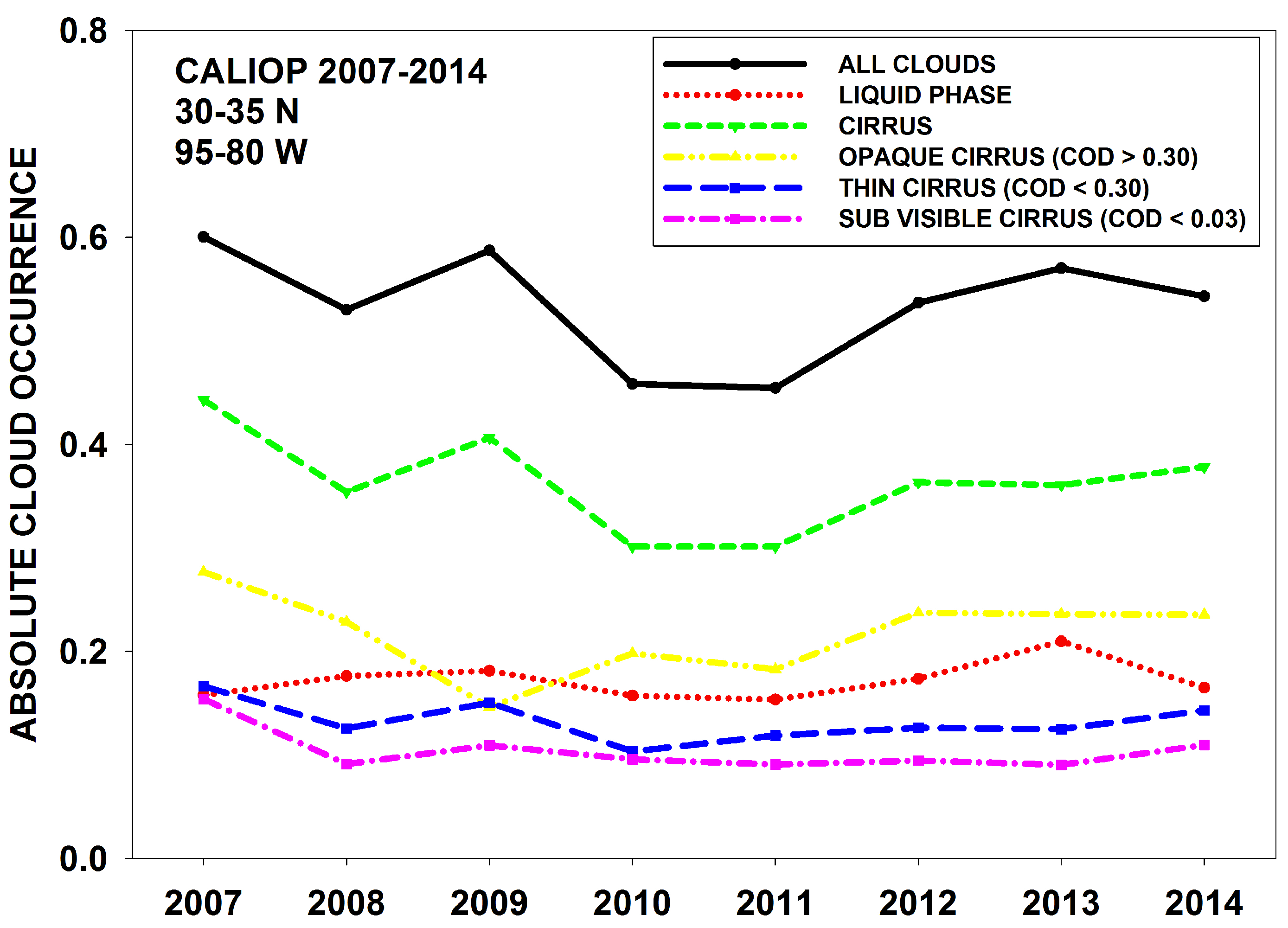
2.2. CALIOP Aerosol Retrievals for 2006–2014

We used version 3.01, 3.02, and 3.30 NASA Cloud Aerosol Lidar with Orthogonal Polarization (CALIOP) Level 2 5-km 532 nm daytime aerosol extinction coefficient data to create summertime-mean (May–September) vertical profiles at 75 m vertical resolution from data collected for 2006–2014. As described in Section 3.1, we restricted our study to the summertime because that was when the warming hole was strongest and when aerosol optical depth was highest. The data were screened for quality assurance using the rubric described by Campbell et al. [38], which very closely mirrors the method described by Winker et al. [39] that is formally endorsed by the CALIPSO (Cloud-Aerosol Lidar and Infrared Pathfinder Satellite Observations project development team. However, the following screening metrics in Campbell et al. [38] improve the robustness of the retrieval method for the purposes of this investigation. First, no profiles were considered if cloud was observed, so as to minimize the corresponding signal attenuation impacting the retrieval of aerosol extinction coefficient in any way. Second, no profiles were considered if the corresponding retrieval failed to resolve aerosol within 250 m of the surface. Finally, profiles were removed if the retrieval failed to observe any aerosol (i.e., aerosol optical depth; AOD = 0). This choice was based on personal communication with Travis Toth (University of North Dakota), and will discussed in a forthcoming publication (which is currently still in preparation). These restrictions as a whole, however, limit the effects of signal attenuation that we believe could compromise the averaged solutions off extinction coefficient profile derived for this study. Approximately 2500 qualifying profiles were averaged each year to construct these profiles. Averages were solved using a Gaussian weighting function to increase the significance of retrievals relative to the center of the 5 ° × 15 ° study domain. We further constructed domain-average CALIOP 532 nm aerosol extinction profiles at 75 m vertical resolution corresponding with each of the native Level 2 species resolved for use in a radiative transfer model experiment described below. Campbell et al. [38], among others, characterize CALIOP AOD and its relative accuracy.
We calculated the total aerosol optical depth (AOD) from the CALIOP data by integrating the extinction coefficient by height. We used atmospheric boundary layer (ABL) data from the ERA (ECMWF Reanalysis) interim [40] to estimate the mean monthly mid-day (1:00 p.m. local time) ABL. We calculated above- (and below) ABL AOD by integrating the extinction coefficient for only that portion of atmosphere that was above (or below) the ERA-estimated noontime ABL height for each month. We also used satellite AOD measurements from the Multi-angle Imaging SpectroRadiometer (MISR) instrument [41] (Version 22, Level 3) for comparison and validation.
Though we note that each seasonally-averaged vertical profile contains approximately 2500 unique CALIOP profiles, we acknowledge that the lower spatial (and temporal) coverage may affect the overall robustness of our analyses, though we anticipate that the overall conclusion to this work is largely unaffected by these limitations.

2.3. Fu–Liou–Gu Radiative Transfer Model

The aerosol direct effect on radiative forcing is investigated using the Fu–Liou–Gu (FLG) model [42,43,44,45]. The vertical profiles used to force the model were constructed from the CALIOP data described above and were taken as a mean extinction at each 75 m layer (the mean of approximately 2500 qualifying profiles per year). An individual profile was created for each aerosol species defined by CALIOP and then matched with the corresponding species in the FLG model. To calculate the net radiative forcing and heating rates for each single species extinction profile, the partial contribution to the total AOD and the value of the species optical depth at each altitude level is required as input for the model.
FLG parameterization uses eighteen different types of aerosols, with single scattering aerosol properties parameterized through the Optical Properties of Aerosol and Clouds (OPAC) catalog [46,47]. However, for our study, four main aerosol types (as defined by CALIOP) contributed more than 95% to the total AOD; these were dust (“transported dust” in FLG), polluted continental (“urban” in FLG), polluted dust (“half urban, half dust" in FLG), and smoke (“black carbon” in FLG). We note the concerns raised by Burton et al. [48] in resolving polluted dust in the Version 3 Level 2 CALIOP algorithms, and concede some measurable offset is introduced here when applying the speciated terms in the manner described. Since we are comparing profiles derived from separate years, however, and our concern focuses on the relative differencing of forcing calculations between the two, our belief is that the uncertainty is self-contained overall and the analysis is ultimately reasonable.
According to Gu et al. [46], the FLG also takes into account the effect of water vapor (available from the standard atmosphere atmospheric profile) on aerosols. We performed two simulations: “pristine”, where the aerosols were excluded (totally clear conditions) and “total sky”, where the individual aerosol species were included. We combined these results into two experiments: FULL, which is simply the “total sky” simulation for each year, and AERO, which is the “total sky” simulation minus the “pristine” simulation for each year. For both experiments, the US1976 standard summer mid-latitude thermodynamics profile was used. Use of the standard atmosphere implies that the water vapor profile was invariant year-to-year. We acknowledge that this is a limitation as water vapor does absorb in the near infrared and that this could impact our direct radiative forcing measurements. However, while we recognize this could cause a small error in our calculations, the data suggest that it does not approach the magnitude of biases derived and discussed or affects the nature of our conclusions.

3. Results and Discussion

3.1. Summertime Warmth Linked to Improved Air Quality

The twentieth century warming hole was especially notable during the summer (Figure 2a) when anthropogenic aerosol concentrations in the SEUS are highest [49]. Summertime temperatures (May–September) in the SEUS decreased by a negligible −0.01 ± 0.35 ° C century 1 between 1900 and 2008, compared with a substantial +0.99 ± 0.35 ° C century 1 increase in Western US (35–48 ° N; 125–110 ° W) temperatures during the same time period (Figure 2c). Time series analysis using LOESS (locally weighted scatterplot smoothing) curve smoothing shows that much of the 20th century decrease in SEUS summertime surface temperature occurred before 1975, plateauing between 1975 and 1990, and with a slight rebound beginning afterward; indeed, the 1900–1975 trend in SEUS surface temperature was a robust −0.27 ± 0.25 ° C century 1 (Figure 3). This period roughly coincided with the peak in SEUS tropospheric aerosol concentration [14].
In recent years, the summertime warming hole has not only disappeared but reversed (Figure 2b). The 2001–2015 temperature trend in the SEUS was +0.54 ± 0.52 ° C decade 1 , compared with +0.18 ± 0.62 ° C decade 1 in the Western US over the same period. Using the alternative Theil–Sen linear trend-fitting algorithm [50], the reversal is still notable and significant, with a positive +0.50 ° C decade 1 trend in SEUS versus a negative −0.18 ° C decade 1 trend in the Western US. When only the most recent decade (2001–2010) is considered, ensuring that the average contains input from all three primary surface temperature records, the contrast is more striking: +0.69 ± 0.68 ° C decade 1 in SEUS and −0.48 ± 0.74 ° C decade 1 in the Western US.
Contemporary (2001–2015) satellite AOD measurements from the Multi-angle Imaging SpectroRadiometer (MISR) instrument [41] (Version 22, Level 3) show high summertime aerosol loading in the SEUS, especially when compared with the Western US where population densities are lower (Figure 4a). Summertime AOD (from MISR) in the SEUS was, on average, 0.05 to 0.10 greater than the long-term annual mean. In contrast, summertime AOD in the Western US was only 0.00 to 0.04 greater during the summer months.
The trend in regionally averaged summertime AOD in the SEUS was −0.05 decade 1 between 2001 and 2015 (Figure 2d, Figure 4b). In contrast, summertime reductions in Western US AOD were minimal, where they existed at all (Figure 4b). Using a bootstrapping technique for error calculation (n = 1,000), we estimate that the 14-year reduction in SEUS AOD was statistically significant (−0.05 ± 0.03). However, a decomposition of the linear trend reveals a sharp drop in AOD between 2007 and 2008. The linear trend from 2001–2007 was near-zero (+0.01 decade 1 ), and the linear trend from 2008 to 2015 was insignificantly negative (−0.03 decade 1 ), suggesting that the majority of the decrease occurred between 2006 and 2009; indeed, the trend from 2005 to 2010 was −0.16 decade 1 . The smoothed curve, fit using LOESS smoothing techniques (n = 5 years), further illustrates this sharp transition. We note that an EPA rules change to the Clean Air Act (CAA) National Ambient Air Quality Standards (NAAQS) for Fine Particulate Matter (PM 2.5 ), implemented beginning in 2006 (Environmental Protection Agency, 40 C.F.R. § 50, 71 FR 2620) corresponds well with the aerosol changes resolved in the data. The rule lowered the 24-h PM 2.5 standard from 65 μ g m 3 to 35 μ g m 3 . That the timing of this rule and its subsequent implementation matches well with the sudden trend reversal represents a circumstantial link that may reconcile the observed relationship [51], though we acknowledge that we have only limited evidence indicating a steep drop in surface-level particulate matter concentration from 2007 to 2009 for several southeast US stations.
The 2001–2015 AOD decrease in the eastern United States (Figure 4b) coincided with a marked increase in average surface temperature (Figure 2d). The spatial correlation of AOD decrease and temperature increase implies that warmer regional temperatures were driven in some manner by improved air quality. To reconcile this relationship, we used vertical profiles of aerosol extinction combined with a one-dimensional radiative transfer model (Section 2.2 and Section 2.3) to assess whether the link could be corroborated quantitatively or was mere coincidental correlation.
Summertime monthly mean profiles of SEUS aerosol light extinction coefficient were derived for 2006–2014 using data from the CALIOP instrument [38] (see Section 2). Similar to our results using MISR, CALIOP data show significant reductions in aerosol burden even over the shorter 2006–2014 time series (Figure 4c). More importantly, CALIOP data show that reductions in aerosol burden were not restricted to the surface layer but persisted as high as 5 km above the surface (though not much higher). The mean summertime (May–September) aerosol extinction coefficient decreased by an average of 35% from 2007 (the first full year of data) to 2014 (Figure 4c). In fact, the mean integrated AOD above the ABL was 41% lower (from 0.13 ± 0.00 to 0.07 ± 0.01) during 2008–2014 when compared with 2006–2007. This contrasts with a 26% reduction for the same time period for the entire tropospheric column (from 0.30 ± 0.02 to 0.23 ± 0.02) (Figure 4c). Furthermore, this decrease was not the result of a positive trend in ABL height, which can enhance the near-surface contribution to total aerosol loading. The ERA interim data show that, while the mean summertime regional ABL experiences interannual fluctuations, the overall trend was neither positive or negative.
Seasonal increases in the amount of secondary aerosols present above the boundary layer in the summer have been proposed to explain the apparent discrepancies noted between the total column aerosol burden from satellites and the measured near-surface pollution reported in EPA pollution measurements [49]. Our data support these findings, but, more notably, the CALIOP data show no apparent trend in aerosol composition from 2007 to 2014, from the surface through the mid-troposphere, indicating a continuity in relative airmass physical properties approaching the surface despite an overall reduction in their relative magnitudes.

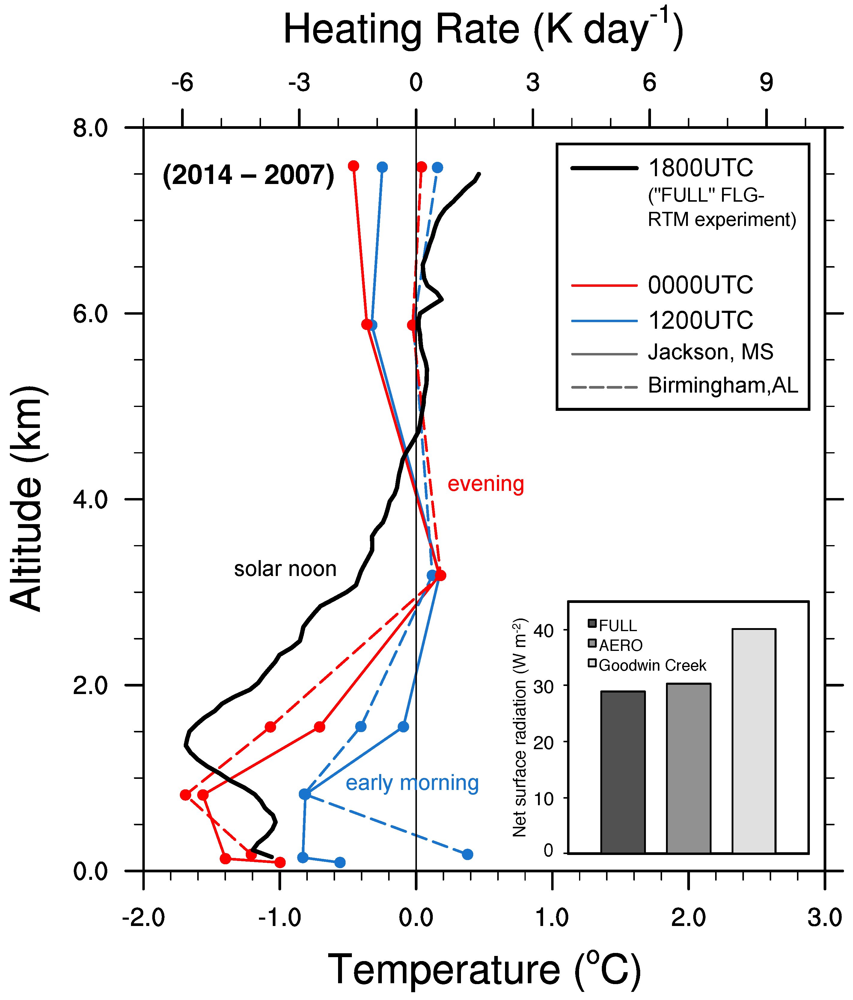
3.2. Modeling Results Corroborate Observations

The FLG radiative transfer model was used to estimate the direct effect of these reductions in aerosol burden on the surface energy budget and column radiative heating profile, and to examine how that effect compares with the observed temperature trends previously discussed. We forced the model (see Section 2.3) with observed changes in vertically-resolved, CALIOP-derived aerosol extinction, broadband surface reflectance from MISR, and standard meteorological conditions, and estimated the direct radiative forcing of the reduced aerosol burden from 2007 to 2014 at solar noon. We performed two experiments, which are described in Section 2.3: FULL (direct forcing effect of aerosols) and AERO (direct forcing effect of aerosols minus a control simulation with no aerosols). Here, we present results from both, but focus on the FULL simulation.
The observed 35% decrease in CALIOP-measured aerosol extinction between 2007 and 2014 resulted in a 29 W m 2 (30 W m 2 for AERO) increase in solar noon net surface energy flux (R n , s r f ) (Figure 5, inset). When we consider the respective CALIOP aerosol profiles for every year (2007 to 2014), the linear trend, which factors in all the intermediate years (2008–2013; see Table 1) in R n , s r f was 2.3 W m 2 year 1 (2.5 W m 2 year 1 for AERO), which, when multiplied by seven (the number of years from 2007 to 2014), was less than the 29 W m 2 absolute difference between 2014 and 2007, but was nevertheless similar. These values are similar to what we derived using an empirical model generated for a Rayleigh-only atmosphere with a direct and diffuse component and gaseous absorption and the observed total column change in AOD (−0.09) [52]. Despite being the average for the entire SEUS, the positive surface energy fluxes also correspond remarkably well with observations from the Goodwin Creek, MS, USA SURFRAD (Surface Radiation Budget Network) 34.25 ° N, 89.87 ° W; https://www.esrl.noaa.gov/gmd/grad/surfrad/goodwin.html) surface radiation monitoring station (Figure 5, inset, Figure 6), which is located in a region of particularly large aerosol reductions (e.g., Figure 4b), is located outside of urbanized area in an area of representative vegetation, and is the only SURFRAD site within our region of interest.
Curiously, while surface energy fluxes increased in the radiative transfer model over the temporal study period, total top of atmosphere (TOA) fluxes decreased between 2007 and 2014: −53.3 W m 2 in the FULL simulation and −50.5 W m 2 in the AERO simulation. As described below, this was probably a result of decreased aerosol absorption in the middle troposphere. In fact, while the trend in TOA radiative forcing was negative, the magnitude was still positive (e.g., 114.8 W m 2 in 2007 to 61.6 W m 2 in 2014 in the FULL simulations).
The FLG-estimated positive change in surface energy flux is a result of less solar absorption and scattering by aerosols in the atmospheric column. In the FULL simulation, lowered aerosol burdens from 2007 to 2014 resulted in a −3.4 K day 1 average decrease in solar noon heating rates between the surface and 4 km (Figure 5). The maximum decrease in heating rates occurred between 0.5 and 2.5 km, corresponding with large observed temperature reductions (2014–2007) at 0.7 km in the temperature sounding data from Birmingham, AL and Jackson, MS (Figure 5). The slight misalignment of the modeled and observed peaks is likely due to differences in the vertical resolution of the sounding data and the model as well as temporal differences; the soundings were taken at 7:00 a.m. (1200 UTC) and 7:00 p.m. (0000 UTC next day) local time, while the model simulations were performed for solar noon (1:00 p.m. local time). Atmospheric heating rates (and, subsequently, temperatures) throughout the lower troposphere were lower in 2014 because the atmospheric aerosol burden was lower. The model results indicate that a decrease in aerosol burden allowed more radiation to reach the surface and atmospheric absorption and semi-direct heating were suppressed. The results are consistent with the observed surface temperature trends, indicating that aerosols played a substantial role in the increasing temperatures observed in this region.

4. Conclusions

In summary, our results show that reduced aerosol direct radiative effects were of sufficient magnitude to contribute to the reversal of negative trends in twentieth century SEUS surface temperature. We present observations from both MISR and CALIOP showing statistically significant decreasing aerosol concentrations both at the surface and at elevated layers from 2007 to 2014 (supplementing results from Attwood et al. [31]). We demonstrate, using reliable profile data and a physically-based model that total column aerosol reductions increase the surface energy flux via direct effects, decrease the column atmospheric heating rate, and act as a probable contribution to an increase in regional surface temperatures since 2001. The consistency of our radiative transfer model results forced with changes in the observed aerosol budget with both surface radiation and atmospheric temperature profile measurements indicates that our results are robust and that the direct influence of aerosols played a significant role in the reversal of the warming hole in the SEUS. We note that Yu et al. [13] find evidence that a substantial portion of the trend reversal may be due to indirect effects. Specifically, they suggest that aerosol effects on shortwave cloud forcing combined with offset from the greenhouse warming of increased water vapor, may explain the temperature trend in SEUS. Our results neither support or contradict this hypothesis and suggest that direct and indirect effects may both play a role in SEUS temperature trends.
The local, direct effect from aerosols is unlikely to explain the entirety of the observed temperature trend reversal, and we acknowledge that the combination of the aerosol forcing with changes in clouds may also play a role. For example, we note significant noise, and relatively low temporal correlation, in both the surface temperature and aerosol trends, suggesting the existence of external mechanisms. Furthermore, Ruckstuhl et al. [53] and Philipona et al. [54] describe a similar rebound in surface temperature trends over mainland Europe in the 1980s as a response to changes in both aerosol burden and cloud distribution—though they note that the change due to direct aerosol forcing greatly outweighed changes from clouds—and our study seemingly validates their results in a different region. Using 2007–2014 cloud fraction data from CALIOP, we find that there is no trend in both total summer cloud fraction (−0.7% ± 1.7%) or liquid cloud fraction (+1.4% ± 1.7) (Figure 7). Similarly, there is no evidence of a trend in monthly cloud fraction or cloud top height anomalies in the MISR data for the same region and a slightly longer time period (Figure 8). While these results do not immediately prove that clouds play no role in the observed temperature trend reversal, they do lend evidence to our analysis that the trend reversal may be driven more directly by changes to atmospheric aerosol burden.
However, while clouds may not have played a role in the reversal of the warming hole, we note that our work only addresses the relative role of aerosol trends. We acknowledge that other factors may also have contributed to positive temperature trends in the SEUS in the twenty-first century (e.g., [55]). In particular, we note that while multi-year trends in AOD and temperature appeared consistent with a direct influence of aerosols on surface temperature, the lack of covariance on interannual timescales suggests that other factors may have been substantial contributors. Our work indicates that aerosols were likely to have played a role in modulating surface temperatures but that other factors—which we did not explicitly account for in this study—may outweigh the aerosol effect. Further investigation of the relative roles of these other factors using a general circulation climate model is a logical next step.
We note that our work does not resolve the larger question of why surface temperatures in the SEUS were particularly sensitive to aerosol trends. While our analysis was restricted to the deep South (where the warming hole was largest), we acknowledge that equally substantial negative AOD trends along the eastern seaboard (Figure 4b) roughly corresponded to positive temperature trends (Figure 2b). Furthermore, extreme warming in eastern Texas did not correspond to equally notable aerosol trends (Figure 2b), suggesting eminent contributions from other meteorological and climatic factors. We also note that while temperature and aerosol trends did co-vary at the regionally-averaged scale, they did not do so at smaller spatial scales; further investigation is necessary to determine why the aerosol effect was not more geographically targeted, though other regional aerosol-specific studies may help elucidate why [56,57]. Going forward, we feel that this work would benefit from the integration of several ground-based observations, including, but not limited to, lidar, ceilometers and photometers. The Aerosol Robotic Network (AERONET), for example, can provide a more direct measure of AOD with potential to characterize aerosol properties, which, when combined with surface radiation measurements, can help elucidate more regionally targeted anomalies [58]. Futhermore, in this work, vertically resolved measurements were critical toward explaining the atmospheric warming and surface radiative response to changing aerosol burden. While the network of ground-based lidar equipment (MPLNET: https://mplnet.gsfc.nasa.gov/) does not currently include data within our study domain, these data are valuable for similar or expanded studies of this problem and further work should attempt to utilize any vertically-resolved aerosol data that may be available now or in the future.
Despite many caveats, this study presents evidence that aerosols played a first-order role in accelerating positive surface temperature trends in the SEUS in recent years. It follows, then, that degraded air quality and aerosol forcing in other regions may similarly be masking climate warming effects within surface temperature records. This is especially true for regions with extremely poor air quality like northern India and eastern China [59,60,61,62]. This study provides contextual evidence for considering aerosol radiative effects and regional cooling when interpreting corresponding surface temperature trends. The logical next step includes characterizing the relative contribution of air quality improvements in the SEUS to increased warming using a regional climate model (such as the Weather Research and Forecasting model); we anticipate running these simulations in the near term.

Acknowledgments

The research included in this manuscript was supported by an ACCDAM grant from the NASA Earth Sciences Division, Radiation Sciences program. We thank the MISR team for providing facilities and useful discussions. We also thank the Naval Research Laboratory for computing facilities. The MISR and CALIOP data were obtained from the NASA Langley Research Center Atmospheric Science Data Center. The links to the temperature datasets are found in Section 2. We also thank Yu Gu (UCLA) for productive conversations and help with the FLG radiative transfer model and Jeffrey Reid (NRL) for productive conversations and suggestions over the past year.

Author Contributions

All authors contributed substantially to this work. All authors performed the research and helped produce the figures. Kalashnikova funded the research and conceived the hypothesis with Tosca, Garay and Campbell. Tosca assembled the paper.

Conflicts of Interest

The authors declare no conflict of interest.

References

  1. Hansen, J.; Ruedy, R.; Sato, M.; Lo, K. Global surface temperature change. Rev. Geophys. 2010, 48, RG4004. [Google Scholar] [CrossRef]
  2. Portmann, R.W.; Solomon, S.; Hegerl, G.C. Spatial and seasonal patterns in climate change, temperatures, and precipitation across the United States. Proc. Natl. Acad. Sci. USA 2009, 106, 7324–7329. [Google Scholar] [CrossRef] [PubMed]
  3. Capparelli, V.; Franzke, C.; Vecchio, A.; Freeman, M.P.; Watkins, N.W.; Carbone, V. A spatiotemporal analysis of U.S. station temperature trends over the last century. J. Geophys. Res. 2013, 118, 7427–7434. [Google Scholar] [CrossRef]
  4. Melillo, J.M.; Richmond, T.C.; Yohe, G.W. Climate Change Impacts in the United States: The Third National Climate Assessment; Technical Report; U.S. Global Change Research Program: Washington, DC, USA, 2014.
  5. Liang, X.Z.; Pan, J.; Zhu, J.; Kunkel, K.E.; Wang, J.X.L.; Dai, A. Regional climate model downscaling of the U.S. summer climate and future change. J. Geophys. Res. 2006, 111, D10108. [Google Scholar] [CrossRef]
  6. Pan, Z.; Arritt, R.W.; Takle, E.S.; Gutowski, W.J., Jr.; Anderson, C.J.; Segal, M. Altered hydrologic feedback in a warming climate introduces a “warming hole”. Geophs. Res. Lett. 2004, 31, L17109. [Google Scholar] [CrossRef]
  7. Meehl, G.A.; Arblaster, J.M.; Branstator, G. Mechanisms contributing to the warming hole and the consequent U.S. East-West differential of heat extremes. J. Climate 2012, 25, 6394–6408. [Google Scholar] [CrossRef]
  8. Robinson, W.A.; Reudy, R.; Hansen, J.E. General circulation model simulations of recent cooling in the east-central United States. J. Geophys. Res. 2002, 107, 4748. [Google Scholar] [CrossRef]
  9. Yu, S.; Saxena, V.K.; Zhao, Z. A comparison of signals of regional aerosol-induced forcing in eastern China and the southeastern United States. Geophs. Res. Lett. 2001, 28. [Google Scholar] [CrossRef]
  10. Shindell, D.; Faluvegi, G. Climate respnose to regional radiative forcing during the twentieth century. Nature Geosci. 2009, 2, 294–300. [Google Scholar] [CrossRef]
  11. Leibensperger, E.M.; Mickley, L.J.; Jacob, D.J.; Chen, W.T.; Seinfeld, J.H.; Nenes, A.; Adams, P.J.; Streets, D.G.; Kumar, N.; Rind, D. Climatic effects of 1950–2050 changes in US anthropogenic aerosols—Part 2: Climate response. Atmos. Chem. Phys. 2012, 12, 3349–3362. [Google Scholar] [CrossRef]
  12. Mickley, L.J.; Leibensperger, E.M.; Jacob, D.J.; Rind, D. Regional warming from aerosol removal over the United States: Results from a transient 2010–2050 climate simulation. Atmos. Environ. 2012, 46, 545–553. [Google Scholar] [CrossRef]
  13. Yu, S.; Alapaty, K.; Mathur, R.; Pleim, J.; Zhang, Y.; Nolte, C.; Eder, B.; Foley, K.; Nagashima, T. Attribution of the United States “warming hole”: Aerosol indirect effect and precipitable water vapor. Sci. Rep. 2014, 4, 6929. [Google Scholar] [CrossRef] [PubMed]
  14. Leibensperger, E.M.; Mickley, L.J.; Jacob, D.J.; Chen, W.T.; Seinfeld, J.H.; Nenes, A.; Adams, P.J.; Streets, D.G.; Kumar, N.; Rind, D. Climatic effects of 1950–2050 changes in US anthropogenic aerosols—Part 1: Aerosol trends and radiative forcing. Atmos. Chem. Phys. 2012, 12, 3333–3348. [Google Scholar] [CrossRef]
  15. Liepert, B.G. Observed reductions of surface solar radiation at sites in the United States and worldwide from 1961 to 1990. Geophys. Res. Lett. 2002, 29, 1421. [Google Scholar] [CrossRef]
  16. Charlson, R.J.; Schwartz, S.E.; Hales, J.M.; Cess, R.D.; Coakley, J.A., Jr.; Hansen, J.E.; Hofman, D.J. Climate forcing by anthropogenic aerosols. Science 1992, 255, 423–430. [Google Scholar] [CrossRef] [PubMed]
  17. Hansen, J.; Sato, M.; Ruedy, R. Radiative forcing and climate response. J. Geophys. Res. 1997, 102, 6831–6864. [Google Scholar] [CrossRef]
  18. Ramanathan, V.; Crutzen, P.J.; Kiehl, J.T.; Rosenfeld, D. Aerosols, climate, and the hydrological cycle. Science 2001, 294, 2119–2124. [Google Scholar] [CrossRef] [PubMed]
  19. Lohmann, U.; Lesins, G. Stronger constraints on the anthropogenic indirect aerosol effect. Science 2002, 298, 1012–1015. [Google Scholar] [CrossRef] [PubMed]
  20. Rosenfeld, D. Aerosols, clouds, and climate. Science 2006, 312, 1323–1324. [Google Scholar] [CrossRef] [PubMed]
  21. Albrecht, B.A. Aerosols, cloud microphysics, and fractional cloudiness. Science 1989, 245, 1227–1230. [Google Scholar] [CrossRef] [PubMed]
  22. Rotstayn, L.D. Indirect forcing by anthropogenic aerosols: A global climate model calculation of the effective-radius and cloud-lifetime effects. J. Geophys. Res. 1999, 104, 9369–9380. [Google Scholar] [CrossRef]
  23. Storelvmo, T.; Leirvik, T.; Lohmann, U.; Phillips, P.; Wild, M. Disentangling greenhouse warming and aerosol cooling to reveal Earth’s climate sensitivity. Nature Geoscience 2016, 9, 206–289. [Google Scholar] [CrossRef]
  24. Mitchell, J.F.B.; Johns, T.C. On modification of global warming by sulfate aerosols. J. Climate 1997, 10, 245–267. [Google Scholar] [CrossRef]
  25. Andreae, M.O.; Jones, C.D.; Cox, p.m. Strong present-day aerosol cooling implies a hot future. Nature 2001, 435, 1187–1190. [Google Scholar] [CrossRef] [PubMed]
  26. Levy, H.; Schwarzkopf, M.D.; Horowitz, L.; Ramaswamy, V.; Findell, K.L. Strong sensitivity of late 21st century climate to projected changes in short-lived air pollutants. J. Geophys. Res. 2008, 113, D06102. [Google Scholar] [CrossRef]
  27. Ming, Y.; Ramaswamy, V. Nonlinear climate and hydrological responses to aerosol effects. J. Clim. 2009, 22, 1329–1339. [Google Scholar] [CrossRef]
  28. Rotstayn, L.D.; Cai, W.; Dix, M.R.; Farquhar, G.D.; Feng, Y.; Ginoux, P.; Herzog, M.; Ito, A.; Penner, J.E.; Roderick, M.L.; et al. Have Australian rainfall and cloudiness increased due to the remote effects of Asian anthropogenic aerosols? J. Geophys. Res. 2007, 112, D09202. [Google Scholar] [CrossRef]
  29. Shindell, D.T.; Faluvegi, G.; Rotstayn, L.; Milly, G. Spatial patterns of radiative forcing and surface temperature response. J. Geophys. Res. 2015, 120, 5385–5403. [Google Scholar] [CrossRef]
  30. Paasonen, P.; Asmi, A.; Petaja, T.; Kajos, M.K.; Aijala, M.; Junninen, H.; Holst, T.; Abbatt, J.P.D.; Arneth, A.; Birmili, W.; et al. Warning-induced increase in aerosol number concentration likely to moderate climate change. Nat. Geosci. 2013, 6, 438–442. [Google Scholar] [CrossRef]
  31. Attwood, A.R.; Washenfelder, R.A.; Brock, C.A.; Hu, W.; Baumann, K.; Campuzano-Jost, P.; Day, D.A.; Edgerton, E.S.; Murphy, D.M.; Palm, B.B.; et al. Trends in sulfate and organic aerosol mass in the Southeast US: Impact on aerosol optical depth and radiative forcing. Geophys. Res. Lett. 2014, 41, 7701–7709. [Google Scholar] [CrossRef]
  32. Kim, P.S.; Jacob, D.J.; Fisher, J.A.; Travis, K.; Yu, K.; Zhu, L.; Yantosca, R.M.; Sulprizio, M.P.; Jimenez, J.L.; Campuzano-Jost, P.; et al. Sources, seasonality, and trends of southeast US aerosol: an integrated analysis of surface, aircraft, and satellite observations with the GEOS-Chem chemical transport model. Atmos. Chem. Phys. 2015, 15, 10411–10433. [Google Scholar] [CrossRef]
  33. Augustine, J.A.; Dutton, E.G. Variability of the surface radiation budget over the United States from 1996 through 2011 from high-quality measurements. J. Geophys. Res. 2013, 118, 43–53. [Google Scholar] [CrossRef]
  34. Tang, Q.; Leng, G. Changes in cloud cover, precipitation, and summer temperature in North America from 1982 to 2009. J. Clim. 2013, 26, 1733–1744. [Google Scholar] [CrossRef]
  35. Zhang, L.; Henze, D.K.; Grell, G.A.; Torres, O.; Jethva, H.; Lamsal, L.K. What factors control the trend of increasing AAOD over the United States in the last decade? J. Geophys. Res. 2017, 122, 1797–1810. [Google Scholar] [CrossRef]
  36. Fan, Y.; van den Dool, H. A global monthly land surface air temperature analysis for 1948-present. J. Geophys. Res. 2008, 113, D01103. [Google Scholar] [CrossRef]
  37. Levi, B.G. Earth’s land surface temperature trends: A new approach confirms previous results. Phys. Today 2013, 66. [Google Scholar] [CrossRef]
  38. Campbell, J.R.; Tackett, J.L.; Reid, J.S.; Zhang, J.; Curtis, C.A.; Hyer, E.J.; Sessions, W.R.; Wetphal, D.L.; Prospero, J.M.; Welton, E.J.; et al. Evaluating nighttime CALIOP 0.532 um aerosol optical depth and extinction coefficient retrievals. Atmos. Meas. Tech. 2012, 5, 2143–2160. [Google Scholar] [CrossRef]
  39. Winker, D.M.; Tackett, J.L.; Getzewich, B.J.; Liu, Z.; Vaughan, M.A.; Rogers, R.R. The global 3-D distribution of tropospheric aerosols as characterized by CALIOP. Atmos. Chem. Phys. 2013, 13, 3345–3361. [Google Scholar] [CrossRef]
  40. Dee, D.P.; Uppala, S.M.; Simmons, A.J.; Berrisford, P.; Poli, P.; Kobayashi, S.; Andrae, U.; Balmaseda, M.A.; Balsamo, G.; Bauer, P.; et al. The ERA-Interim reanalysis: configuration and performance of the data assimilation system. Q. J. R. Meteorol. Soc. 2011, 137, 553–597. [Google Scholar] [CrossRef]
  41. Martonchik, J.V.; Diner, D.J.; Crean, K.A.; Bull, M.A. Regional aerosol retrieval results from MISR. IEEE Trans. Geosci. Remote Sens. 2002, 40, 1520–1531. [Google Scholar] [CrossRef]
  42. Fu, Q.; Liou, K.N. On the correlated k-distribution method for radiative transfer in nonhomogeneous atmospheres. J. Atmos. Sci. 1992, 49, 2139–2156. [Google Scholar] [CrossRef]
  43. Fu, Q.; Liou, K.N. Parametrization of the radiative properties of cirrus clouds. J. Atmos. Sci. 1993, 50, 2008–2025. [Google Scholar] [CrossRef]
  44. Gu, Y.; Farrara, J.; Liou, K.N.; Mechoso, C.R. Parametrization of cloud-radiative processes in the UCLA general circulation model. J. Climate 2003, 16, 3357–3370. [Google Scholar] [CrossRef]
  45. Gu, Y.; Liou, K.N.; Ou, S.C.; Fovell, R. Cirrus cloud simulations using WRF with improved radiation parametrization and increased vertical resolution. J. Geophys. Res. 2011, 116, D06119. [Google Scholar] [CrossRef]
  46. Gu, Y.; Liou, K.N.; Jiang, J.H.; Su, H.; Liu, X. Dust aerosol impact on North African climate: A GCM investigation of aerosol-cloud-radiation interactions using A-Train satellite data. Atmos. Chem. Phys. 2012, 12, 1667–1679. [Google Scholar] [CrossRef]
  47. Hess, M.; Koepke, P.; Schult, I. Optical properties of aerosols and clouds: The software package OPAC. Bull. Am. Meteor. Soc. 1998, 79, 831–844. [Google Scholar] [CrossRef]
  48. Burton, S.P.; Ferrare, M.A.; Vaughan, A.H.; Omar, A.H.; Rogers, R.R.; Hostetler, C.A.; Hair, J.W. Aerosol classification from airborne HSRL and comparisons with the CALIPSO vertical feature mask. Atmos. Meas. Tech. 2013, 6, 1397–1412. [Google Scholar] [CrossRef]
  49. Ford, B.; Heald, C.L. Aerosol loading in the Southeastern United States: Reconciling surface and satellite observations. Atmos. Chem. Phys. 2013, 13, 9269–9283. [Google Scholar] [CrossRef]
  50. Theil, H. A rank-invariant method of linear and polynomial regression analysis. I. Nederl. Akad. Wetensch. Proc. 1950, 53, 386–392. [Google Scholar]
  51. Hand, J.L.; Schichtel, B.A.; Malm, W.C.; Pitchford, M.L. Particulate sulfate ion concentration and SO2 emissions trends in the United States from the early 1990s through 2010. Atmos. Chem. Phys. 2012, 12, 10353–10365. [Google Scholar] [CrossRef]
  52. Gregg, W.W.; Carder, K.L. A simple spectral solar irradiance model for cloudless maritime atmospheres. Limnol. Oceanog. 1990, 35, 1657–1675. [Google Scholar] [CrossRef]
  53. Ruckstuhl, C.; Philipona, R.; Behrens, K.; Coen, M.C.; Durr, B.; Heimo, A.; Matzler, C.; Nyeki, S.; Ohmura, A.; Vuilleumier, L.; et al. Aerosol and cloud effects on solar brightening and the recent rapid warming. Geophys. Res. Lett. 2008, 35, L12708. [Google Scholar] [CrossRef]
  54. Philipona, R.; Behrens, K.; Ruckstuhl, C. How declining aerosols and rising greenhouse gases forced rapid warming in Europe since the 1980s. Geophys. Res. Lett. 2009, 36, L02806. [Google Scholar] [CrossRef]
  55. Meehl, G.A.; Arblaster, J.M.; Chung, C.T.Y. Disappearance of the southeast U.S. “warming hole” with the late 1990s transition of the Interdecadal Pacific Oscillation. Geophys. Res. Lett. 2015, 42, 5564–5570. [Google Scholar] [CrossRef]
  56. Che, H.; Xia, X.; Zhu, J.; Dubovnik, O.; Holben, B.; Goloub, P.; Chen, H.; Estelles, V.; Cueas-Agullo, E.; Blarel, L.; et al. Column aerosol optical properties and aerosol radiative forcing during a serious haze-fog month over North China Plain in 2013 based on ground-based sunphotometer measurements. Atmos. Chem. Phys. 2014, 14, 2125–2138. [Google Scholar] [CrossRef]
  57. Prats, N.; Cachorro, V.E.; Berjon, A.; Toledano, C.; De Frutos, A.M. Column-integrated aerosol microphysical properties from AERONET Sun photometer over southwestern Spain. Atmos. Chem. Phys. 2011, 11, 12535–12547. [Google Scholar] [CrossRef]
  58. Holben, B.N.; Eck, T.F.; Slutsker, I.; Tanre, D.; Buis, J.P.; Setzer, A.; Vermote, E.; Reagan, J.A.; Kaufman, Y.; Nakajima, T.; et al. AERONET-A federated instrument network and data archive for aerosol characterization. Remote Sens. Environ. 1998, 66, 1–16. [Google Scholar] [CrossRef]
  59. Donkelaar, A.V.; Martin, R.V.; Brauer, M.; Kahn, R.; Levy, R.; Verduzco, C.; Villeneuve, P.K. Global estimates of ambient fine particulate matter concentrations from satellite-based aerosol optical depth: Development and application. Environ. Health. Perspect. 2010, 118, 847–855. [Google Scholar] [CrossRef] [PubMed]
  60. Li, P.; Yan, R.; Yu, S.; Wang, S.; Liu, W.; Bao, H. Reinstate regional transport of PM2.5 as a major cause of severe haze in Beijing. Proc. Natl. Acad. Sci. USA 2015, 112, E2739–E2740. [Google Scholar] [CrossRef] [PubMed]
  61. Yan, R.; Yu, S.; Zhang, Q.; Li, P.; Wang, S.; Chen, B.; Liu, W. A heavy haze episode in Beijing in February of 2014: Characteristics, origins and implications. Atmos. Pollut. Res. 2015, 6, 867–876. [Google Scholar] [CrossRef]
  62. Yu, S.; Li, P.; Wang, L.; Wang, P.; Wang, S.; Chang, S.; Liu, W.; Alapaty, K. Anthropogenic aerosols are a potential cause for migration of the summer monsoon rain belt in China. Proc. Natl. Acad. Sci. USA 2016, 11, E2209–E2210. [Google Scholar] [CrossRef] [PubMed]
Figure 1. Time series of mean annual temperature anomalies for the southeast US (solid lines; 30–35 ° N, 95–80 ° W) and the continental US (dashed lines; 25–50 ° N, 125–65 ° W). For panel (a), the unique colors represent three independent gridded temperature datasets–red = Delaware, black = GHCN and blue = Berkeley; For panel (b), the lines are each respective region’s mean temperature anomaly, averaged across all three datasets in (a). The trend lines in (b) are linear trends of temperature anomalies from 1900–2008, with error estimates, calculated using bootstrapping techniques (n = 1000), shown as the solid shaded regions.
Remotesensing 09 00674 g001
Figure 2. (a) linear trends in summer (May–September) surface temperatures from the Delaware dataset for 1900–2008 (0.5 degree resolution); (b) linear trends in summer surface temperatures from the Berkeley dataset for 2001–2015 (one-degree resolution). Stipling indicates statistically significant trends at 95% confidence; (c) regionally averaged summer surface temperature anomalies for 1850–2015 for the Southeast US (black) and the Western US (red) (regions defined by boxes in (a,b)). Linear trends for 1900–2008 (dashed lines) and 2001–2015 (solid lines) are noted; (d) summertime surface temperature and aerosol optical depth (AOD) anomalies for the southeast US for 1990–2015. The 2001–2015 linear trend is noted by solid lines. Error estimates calculated using the bootstrapping method (n = 1000) are shown as shaded solids.
Remotesensing 09 00674 g002
Figure 3. Time series of the 1900 to “year” linear trend (least-squares) for each “year” from 1960 to 2015. The green shaded region represents the error estimate (95% confidence) of the linear trend. Note the negative trends for the time period ranging from 1900 to 1970 through the time period ranging from 1900 to 2010, and the recent flip to positive trends after 2010.
Remotesensing 09 00674 g003
Figure 4. (a) summertime (May–September) aerosol optical depth (AOD) averaged for 2001–2015; (b) the linear trend (2001 to 2015) in summertime AOD. Aerosol data were taken from MISR (Multi-Angle Imaging Spectroradiometer) Stipling indicates statistically significant trends at 95% confidence; (c) main: vertical profiles of average summertime (May–September) aerosol extinction coefficients (km 1 ) in the southeast US (SEUS) for both 2007 and 2014 calculated using CALIOP (Cloud Aerosol Lidar Orthogonal Polarization) lidar data. inset: summertime SEUS aerosol optical depth (AOD) averages for two periods (2000*–2007 and 2008–2014). CALIOP_total = total column AOD from the CALIOP instrument; CALIOP_elev = only elevated AOD (above the boundary layer) from the CALIOP instrument and MISR = MISR total column AOD. * For the two CALIOP variables: 2006–2007.
Remotesensing 09 00674 g004
Figure 5. main: vertical profiles of the difference (2014–2007) in heating rates (thick black line) and atmospheric temperatures (red and blue lines) in SEUS from the ’FULL’ FLG-RTM (Fu-Lio-Gu Radiative Transfer Model) model experiment (black line) at solar noon (1800 UTC) and atmospheric sounding data from Birmingham, AL, USA (dashed lines) and Jackson, MS, USA (solid lines) at 8:00 a.m. local time (1200 UTC) and 8:00 p.m. local time (0000 UTC). inset: net surface radiation differences (2014 minus 2007) at solar noon from the ‘FULL’ and ‘AERO’ (see Section 2.3) FLG-RTM experiments and the integrated 1700–1900 UTC average from the Goodwin Creek, MS, USA SURFRAD (surface radiation) measuring station. Goodwin Creek values were computed by pairing the number of days and the times so that the intrinsic sampling was identical.
Remotesensing 09 00674 g005
Figure 6. A diurnal time series of average summertime (May–September) direct minus normal surface radiation received at Goodwin Creek, MS, USA for 2007 (pink) and 2014 (yellow).
Remotesensing 09 00674 g006
Figure 7. CALIOP-derived cloud fraction over the Southeast US (SEUS) for 2007 through 2014 showing no evident trend during the period.
Remotesensing 09 00674 g007
Figure 8. MISR-derived monthly cloud fraction over the Southeast US (SEUS) for March 2000 through 2015 showing no evident trend during the period. The thick gray line represents the anomaly in the mean cloud height smoothed with a 12-month running mean. The actual data are in blue and the gray lines indicate the 1-sigma bounds. The thick green line is the cloud fraction anomaly.
Remotesensing 09 00674 g008
Table 1. Fu-Liou-Gu (FLG) radiative transfer model reported net surface forcing values for each simulation.
YearNet, Noontime Forcing (W m 2 )
FULLAERO
2007−50.3460.1
2008−29.4480.9
2009−29.0483.9
2010−35.4477.3
2011−30.2483.7
2012−28.1484.2
2013−32.8478.1
2014−21.3490.4
Trend (year 1 )+2.30+2.45

