1. Introduction
Aerosols and clouds influence the Earth’s radiation budget, as do intermediate stages of hydrated aerosol-cloud mixtures in the space between both features [
1]. Magnitude and mechanisms of these radiative effects and their impact on the global climate system are still highly uncertain, including direct radiative effects of aerosols, as well as their various interactions with clouds, believed to alter cloud reflectivity, lifetime and precipitation susceptibility [
1,
2,
3,
4]. While global-scale observation-based studies of aerosol-cloud interactions commonly focus on regions with fairly homogeneous aerosol or cloud, large transition regions exist. These transition zones have been called a “continuum” [
5] or a “twilight zone” [
1], and are the focus of this study. For a better understanding of aerosol-cloud interactions, it is necessary to comprehend the extent and spatial patterns of this transition zone between aerosols and clouds and its impact on the Earth’s energy balance [
1,
6,
7]. Accordingly, the transition zone between aerosols and clouds has received increasing attention, and is influenced radiatively by the presence of activated aerosols and nearby optically thick clouds [
1,
5].
Satellite-based retrievals of aerosol and cloud properties are error-prone in these transition zones [
6]; as a measure to ensure an adequate quality of cloud and aerosol property products, any regions not identified as cloudy or clear with high certainty are left out in the cloud and aerosol retrieval procedures, respectively [
6,
8,
9]. Due to this, transition regions between aerosols and clouds are largely absent from studies relying on large-scale observations data sets. As shown by Fuchs and Cermak [
10], nearly six percent of CALIPSO lidar atmospheric profiles fall into this category. Since observation-based studies of aerosols, clouds, and aerosol–cloud interactions focus on areas where aerosol and cloud products are available. Previous studies focus on thresholds of reflectances for retrieval calculations or on the reasons for retrieval failure [
6,
8], but little is known about the role of the transition zone or its radiative properties. This study aims to bridge this knowledge gap by specifically focusing on the locations and properties of this zone.
The goal of this study is to locate, quantify and characterize pixels in products derived from measurements by the Moderate-Resolution Imaging Spectro-Radiometer (MODIS) instrument. In particular, the focus is on regions identified neither as clouds nor as aerosols or clear and clean areas. These regions are assumed to represent the transition zone between aerosols and clouds. The occurrence frequency and the reflective properties of these pixels are analyzed in order to compare them to those of clouds and aerosols. A distance function to the nearest cloud and the nearest aerosol is utilized to explain the importance of these pixels in the context of aerosol-cloud interactions.
2. Data and Methods
The products of the Moderate-Resolution Imaging Spectro-Radiometer (MODIS) sensor aboard the Aqua satellite are employed in this study. The global analysis considers all available February and August data of five years (2007–2011) of the Collection 6 daytime ocean products. Products included are the 1 km geolocation product (MYD03), 0.645
m reflectance from the Level 1 radiance data product (MYD021KM) at 1 km resolution, the Aerosol-Cloud-Mask (ACM) taken from the Level 2 Aerosol product (MYD04) at 500 m resolution, the Cloud Optical Depth (COD) from the Level 2 Cloud product (MYD06) at 1 km resolution, and the Cloud Mask (CM) product (MYD35) at 1 km resolution [
11,
12,
13,
14,
15]. All scenes within the period with all of the MODIS ocean products available are considered for the analysis. Only ocean products are considered for the analysis, in order to minimize the retrieval failure due to the difficulties in cloud masking over land [
11]. The MYD35 cloud mask identifies clear pixels and, using a series of spatial tests assigns the remainder to classes of cloud and other obstructions [
11,
13,
16,
17].
The ACM classifies clear and cloudy pixels based on an analysis of reflectances in pixel environments [
6]. For comparability with the other products, the ACM is resampled from its original 500 m grid to the 1 km grid of the other data sets. For each 1 km pixel, a weighted reassignment is performed on the basis of the eight relevant 500 m subpixels [
18]. The most frequent value (“cloud” or “clear”) is chosen for the aerosol classification [
12]. Here, clear pixels describe the cloud-free areas, which are considered for the aerosol property retrievals [
11]. In this study, the threshold of 50%, where 50% of the ACM pixels have to be covered by cloud or clear, is chosen because stricter thresholds result in a high loss of data, e.g., a threshold of 100% would result in no values in the aerosol class, whose values then are assigned predominantly to the clear class (nearly 98%). Generally, the spatial distribution of clouds is more variable than that of aerosols [
19]. For this reason, low thresholds in the interpolation procedure are expected to result in adequate allocations.
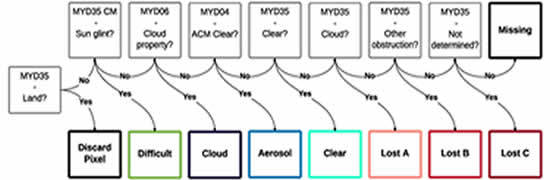
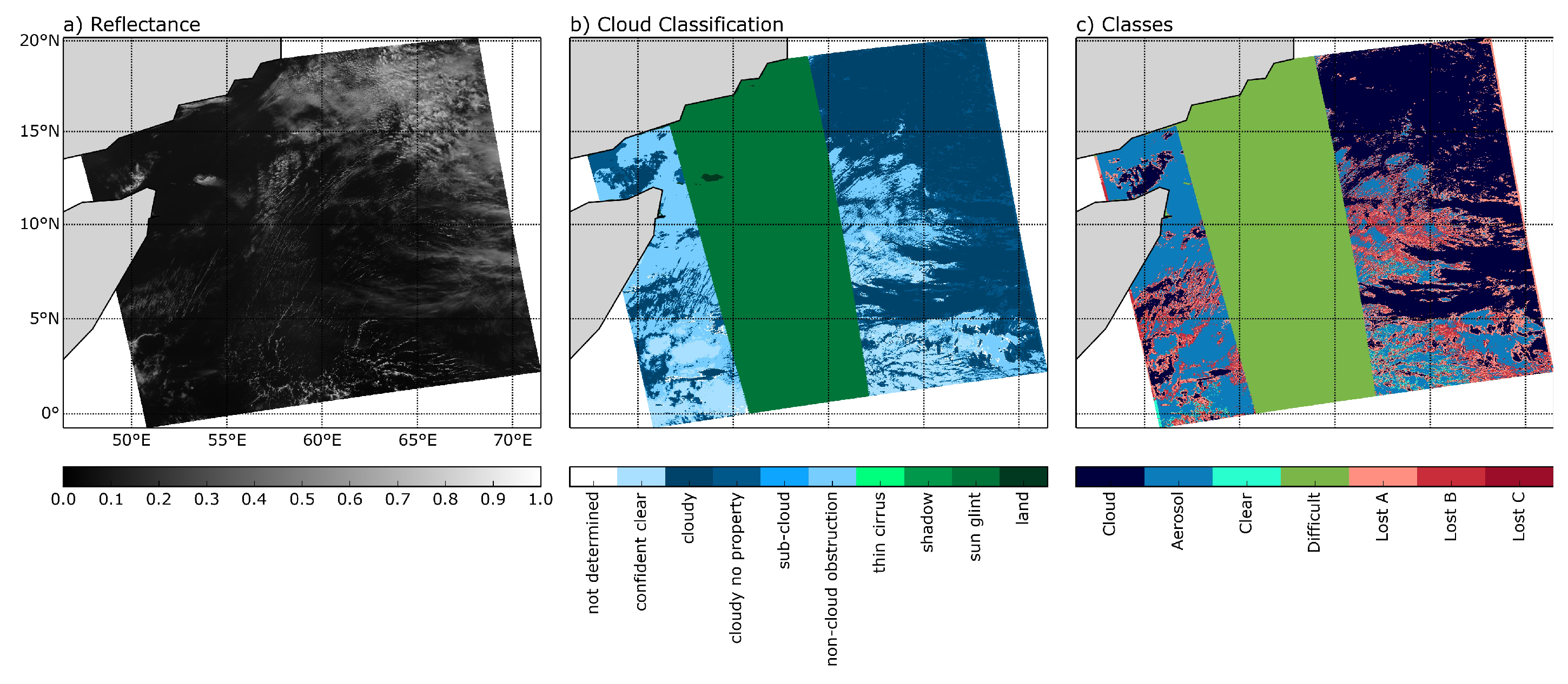
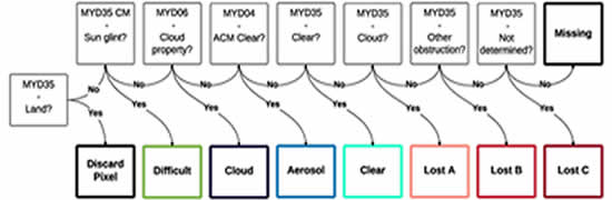
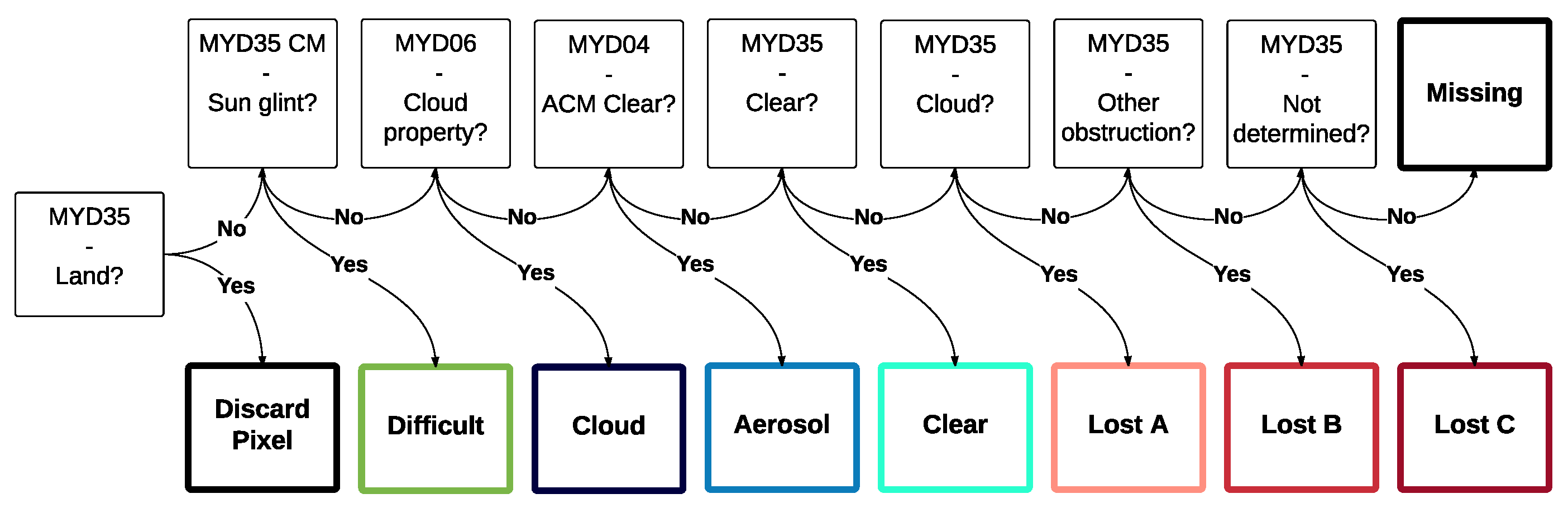
After all data sets have been transferred to the same 1 km grid, all pixels with a solar zenith angle >90° are discarded. In order the identify the lost pixels between pure aerosol and pure cloud regions, specific properties are tested for in the MODIS products in the sequence shown in
Figure 1. The following classes of pixels result from this procedure: “Difficult”, “Cloud”, “Aerosol”, “Clear”, “Lost A”, “Lost B”, “Lost C” (
Figure 2c). The three “Lost” classes are intended to encompass separate subsets of the lost pixel regions, as shown in
Figure 1.
When all classes containing cloud, aerosol, clear area or sun glint are taken together, the lost pixels are what remains. For these pixels neither aerosol nor cloud retrievals exist, still they are classified as containing a cloud (Lost A), a non-cloud obstruction (Lost B), or were not processed at all in the cloud masking (Lost C), as shown in
Figure 1. Non-cloud obstructions could be an aerosol-laden atmosphere characterized by smoke, biomass burning or dust aerosol [
11]. The Cloud Mask retrieval fails where all the radiance values used in the cloud mask are missing or outside the permitted range [
11] or due to geolocation problems [
20]. An example scene classified in this way is shown in
Figure 2.
For all pixels belonging to each class, reflectance information is extracted from the 0.645
m channel measurements as shown in the sample scene in
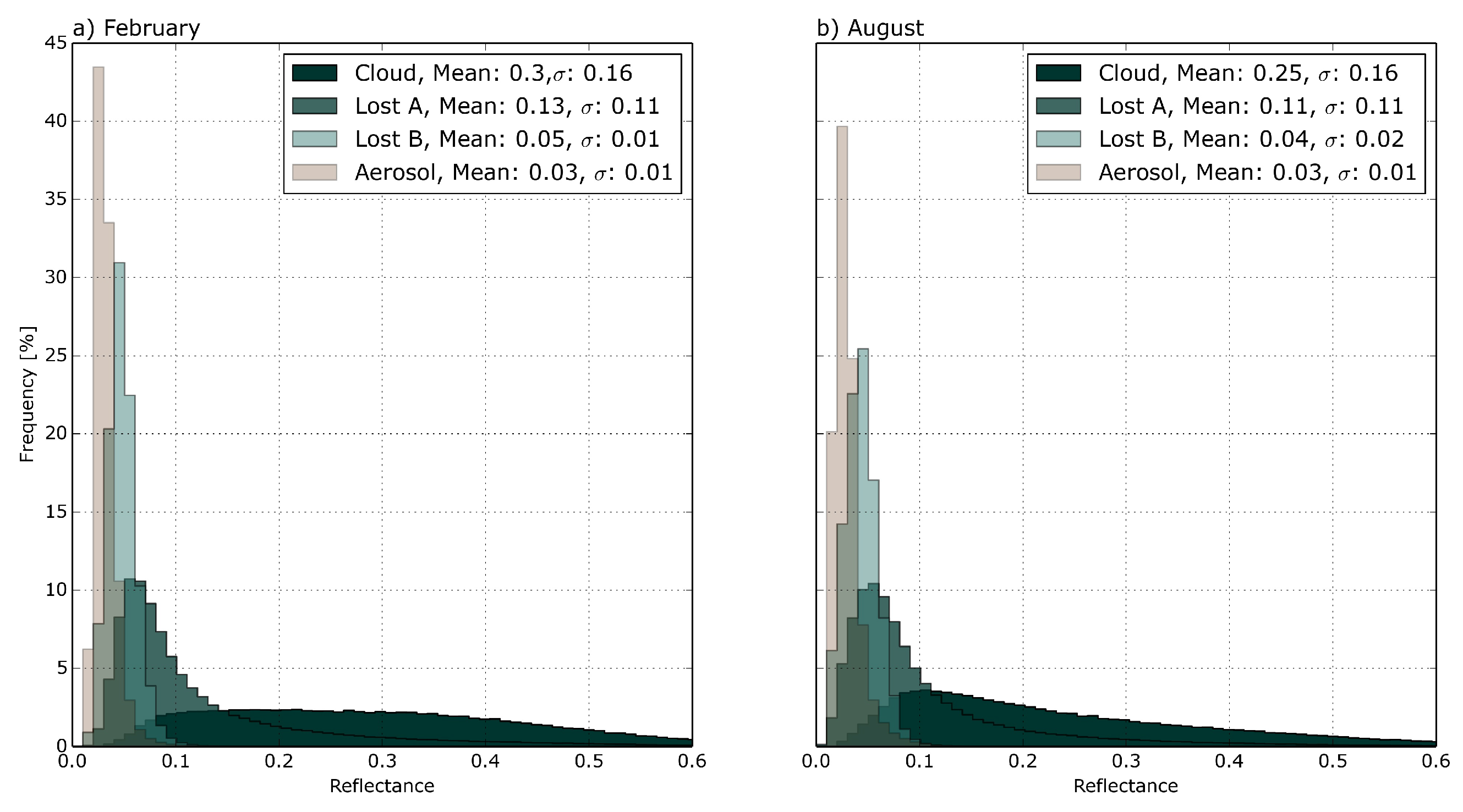
Figure 2a. In order to harmonize sample sizes for the classes, random samples of 500,000 data points are chosen for each class, evenly distributed over all five years with 100,000 data points for each February and August. A summary of the reflective properties of these samples for the classes Cloud, Lost A, Lost B and Aerosol is shown in
Figure 3 with mean values and standard deviations, respectively.
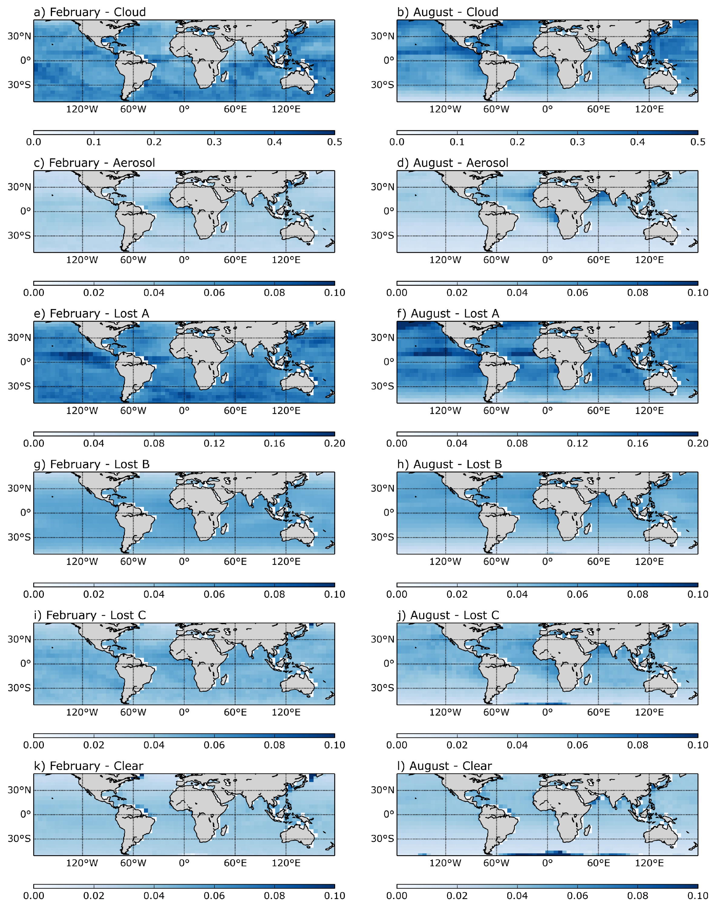
In addition to the reflective properties, the frequency distribution of each class is also assessed on a spatial grid of 5
× 5
for mapping the considered classes (
Figure 4 and
Figure 5). Exemplary, for August 2007, median reflectances and frequencies of the Lost Pixel classes are analyzed as a function of distance in kilometers to the nearest cloud or aerosol pixel to strengthen the relation to these. The results for the other times are very similar and therefore not further included.
The analysis is done on a global scale for February and August from 2007 to 2011. By comparing these months, the seasonal differences in aerosol and cloud dynamics are considered, which are, induced by the shift of the inner-tropical convergence zone (ITCZ), seasonal differences in biomass burning, or dust aerosols [
2,
21,
22,
23].
3. Results
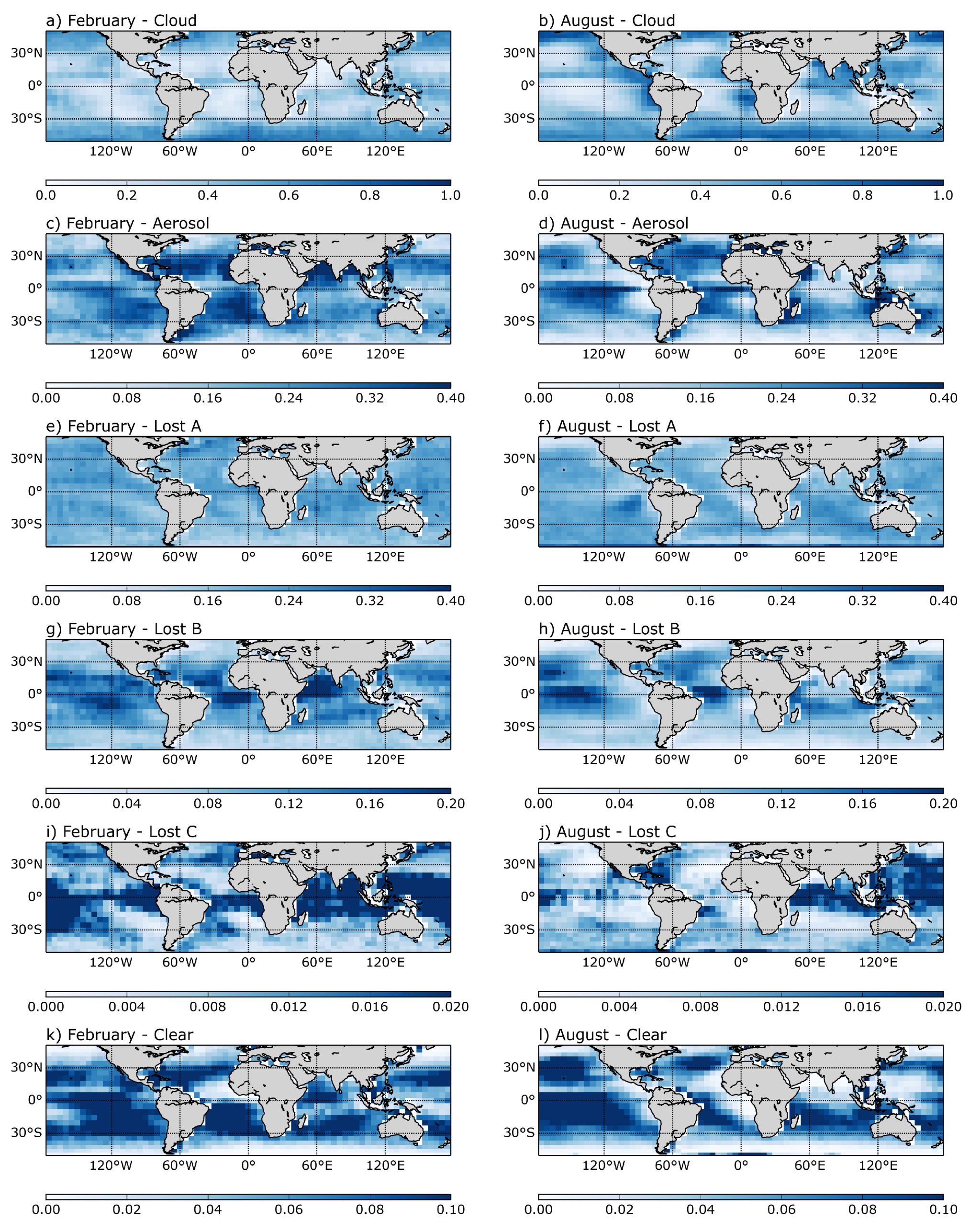
Figure 4 shows the global distribution of the occurrence frequency of all classes, as the ratio of amount of the pixels of each class and all pixels, for February and August respectively. Within each month, the spatial frequency distributions of classes are complementary, in particular the locations of cloud and aerosol classes (
Figure 4a–d). Examples of note are the South-East Atlantic region in August, and the ITCZ in both months indicated by the increased cloud occurrence frequency (
Figure 4a,b).
Average reflectances of the classes (
Figure 5) show generally high values for clouds. Especially high cloud reflectances are located in the ITCZ (
Figure 5a,b), and in August in the recurrent stratocumulus cloud decks as the dominant cloud type in the South-East-Atlantic, as well as in the South-East-Pacific (
Figure 5b) [
23]. High aerosol loadings are found in the area influenced by Saharan dust, west of the West-African coast, as well as in the South-East-Atlantic region, where biomass-burning aerosol is prevalent (
Figure 4c,d). The reflectances of the class Lost A (
Figure 5e) display a spatial pattern similar to that of clouds (
Figure 5a). The classes Lost B (
Figure 5g) and Lost C (
Figure 5i) are comparable to the aerosol class (
Figure 5c).
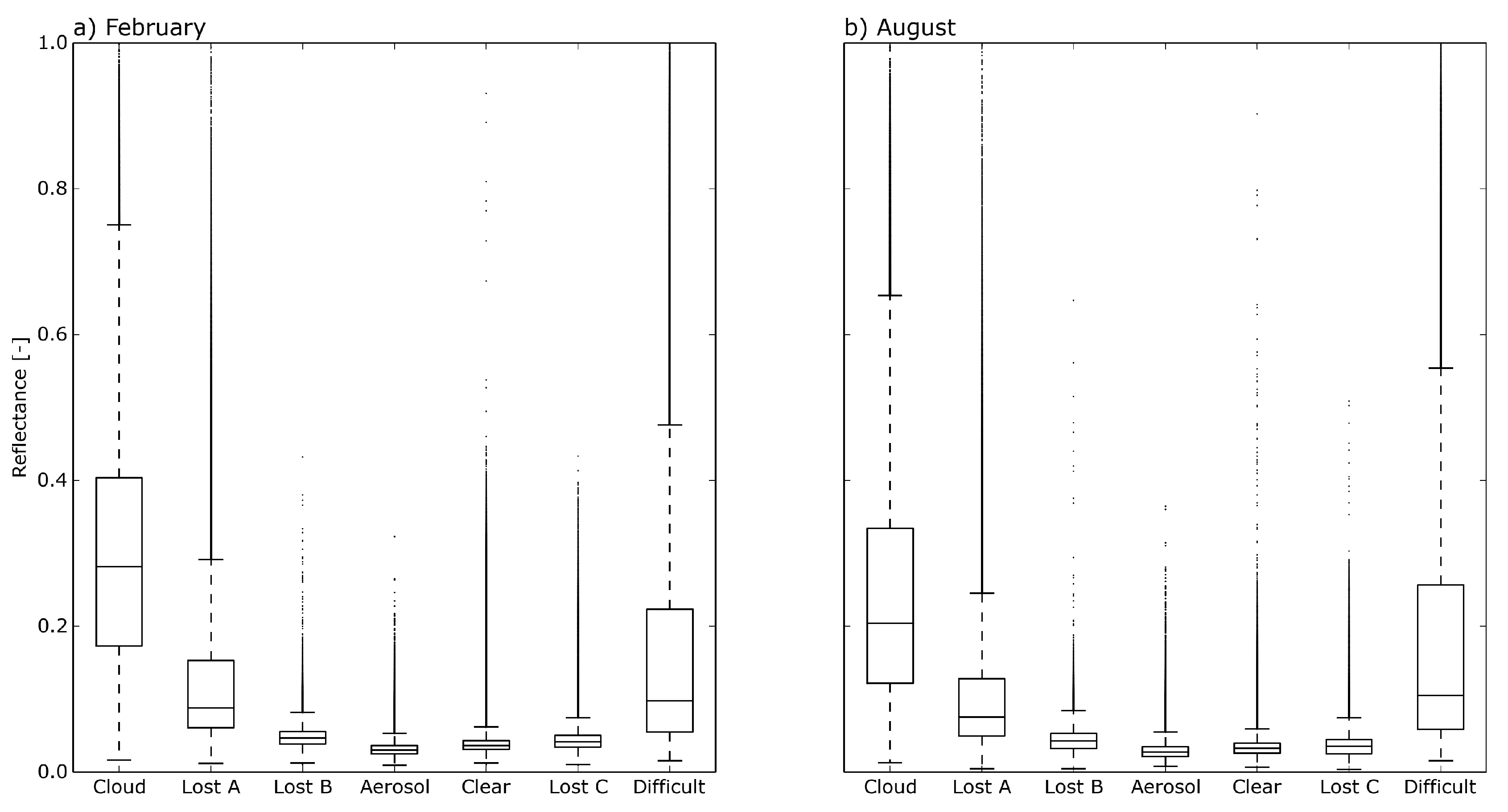
The reflective properties of all classes are summarized globally in
Figure 6. As expected, pixels of the “Cloud” class generally have the highest reflectances, while aerosol pixels have lower ones. The “Lost” classes are in between the properties of clouds and aerosols, as already depicted in the global mean reflectance maps (
Figure 5). The reflective properties of Lost A are closer to those of clouds than the other two “Lost” classes.
4. Discussion
The classification of the satellite-derived data using the approach shown in
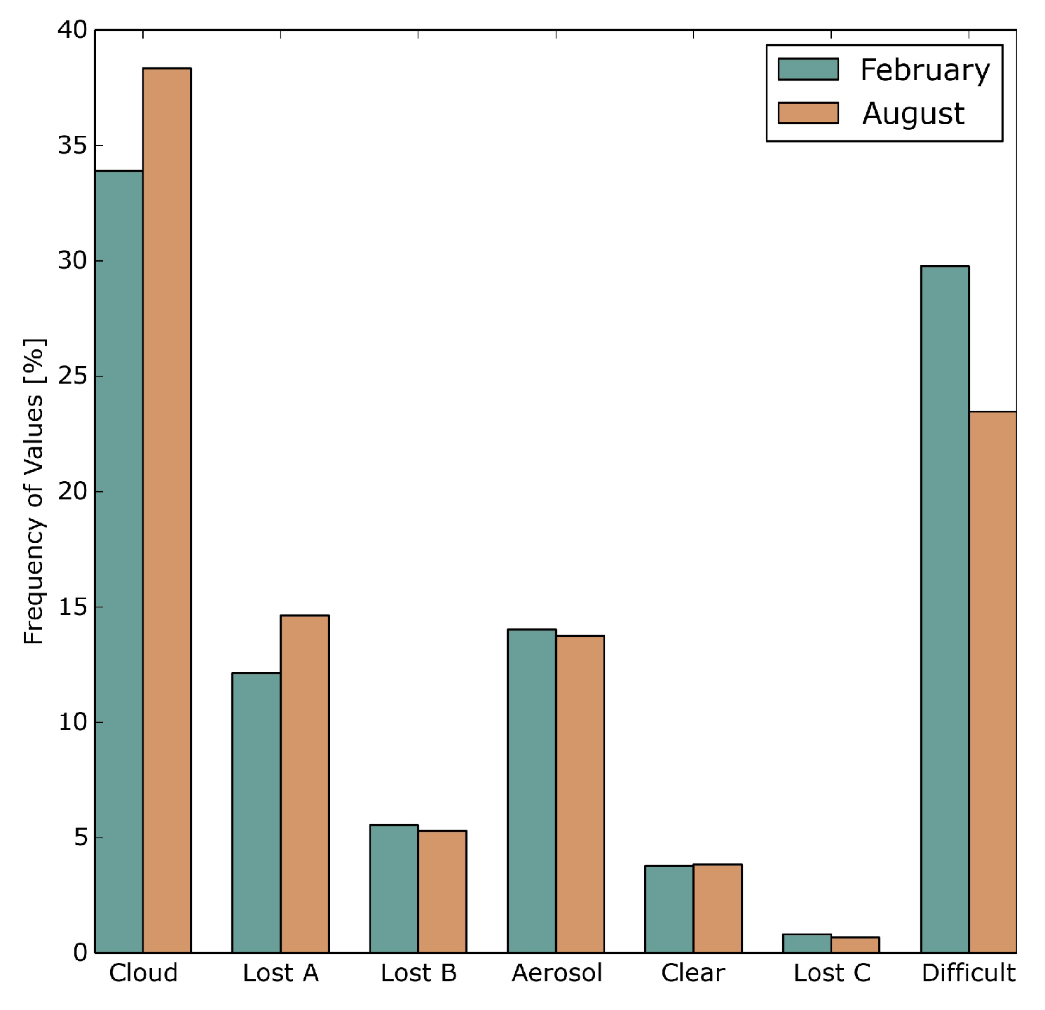
Figure 1 resulted in classes with distinctly different reflective properties. About a fifth of all data points are classified into one of the “Lost” categories in both months analyzed, and over all years (
Figure 7). Consequently, only about 80% of all data points are considered in the retrieval calculations for aerosol and cloud detection (
Figure 7). The reflective properties of the “Lost” pixels are distributed in the intermediate range between aerosol and cloud reflectances (
Figure 3 and
Figure 6). This likely indicates that “Lost” pixels to a large degree represent intermediate stages between or mixtures of aerosols and clouds.
“Lost A” pixels (February: 12.1% of all observations, August: 14.6% of all observations) are identified as cloud pixels by the MYD35 CM, but there are no cloud property products available. An analysis by Cho et al. [
8] suggests that some of these may be explained by spectral characteristics outside the algorithm definitions. One explanation is the presence of cloud halo pixels in Lost A, which are characterized by increasing reflectance with increasing proximity to a pure cloud pixel [
1,
7,
9,
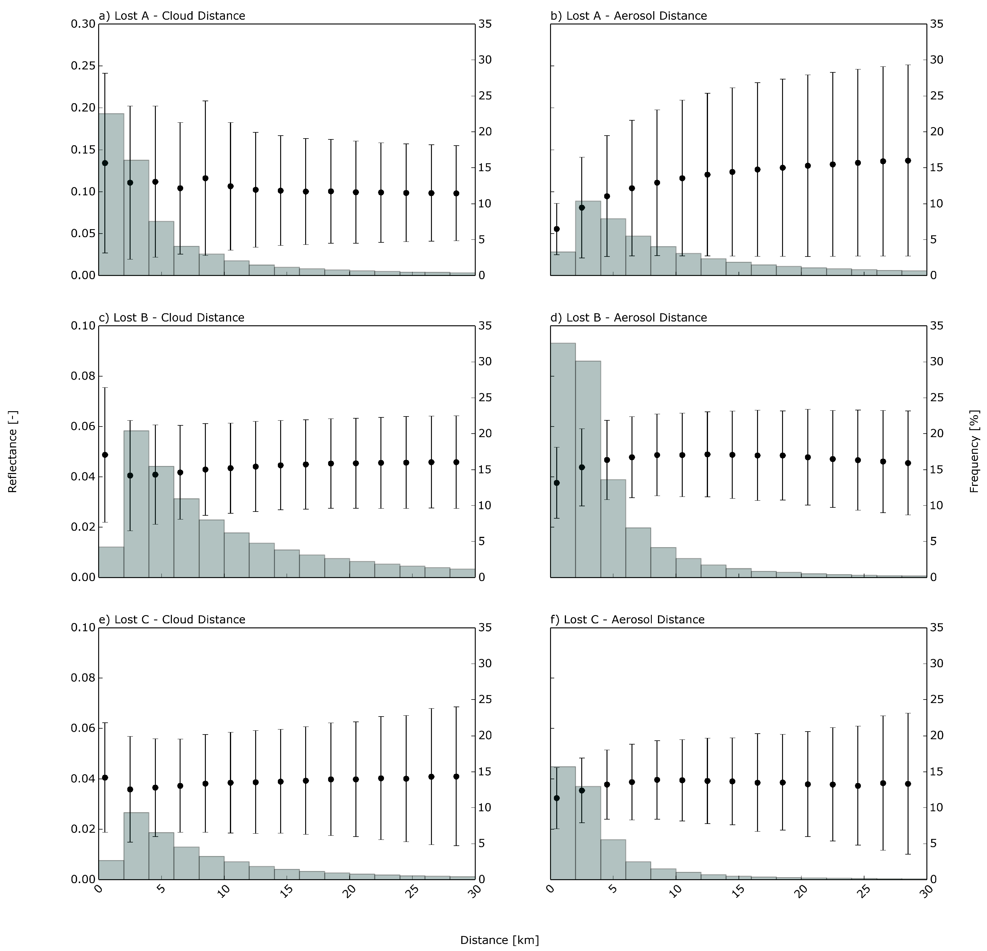
24]. Indeed, the analysis of class reflectivities as a function of distance from cloud and aerosol features as shown in
Figure 8 supports this: Most of the values with the highest reflectivities in “Lost A” are close to the nearest cloud, as shown in
Figure 8a, with opposite conclusions for the aerosol pixels with increasing reflectivity with larger distances (
Figure 8b). Accordingly, the spatial distribution of the higher mean reflectances of the class ‘Lost A’ shows patterns very similar to the “Cloud” class. In particular, the ITCZ is prominent in both maps (
Figure 5a,b,e and
Figure 6f). Thus, “Lost A” can be seen to depict the gradual reduction of reflectance from a cloudy to a humid cloud-free atmosphere, probably made up of evaporating cloud fragments and cloud halos [
1,
24].
The reflectance of class “Lost B” (5% in February and August) is fairly homogeneous globally, as shown in
Figure 5g,h. The properties of these pixels are in the range between the “Lost A” pixels and the “Aerosol” pixels (
Figure 6). It can be speculated that these pixels are partly hydrated aerosols, which represent the cloud formation process, or thin clouds [
1,
10]. Striking is the slightly increased reflectivity in regions with high aerosol loading, e.g., the South-East Atlantic or the Arabian Sea in August or the windblown Saharan dust in February over the Atlantic Ocean (
Figure 5g) [
25]. Additionally, the decreasing reflectance with larger distances, as well as higher frequencies at higher distances to the nearest cloud in comparison with class “Lost A”, indicate that these pixels are not directly influenced by clouds (
Figure 8c), but aerosol swelling alters the reflective properties. This class is characterized by the presence of aerosols, but there are no aerosol retrievals. This is underlined by the increased reflectances found in Lost B in the immediate surroundings of aerosol pixels, as seen in
Figure 8d.
The class “Lost C”, with a global fraction of nearly 1% in February and August, represents pixels where retrievals are impossible for a range of reasons other than the physical phenomena contained in the other classes (see above). Striking patterns are the reflective properties and the global distribution, especially in regions of high aerosol loadings, e.g., the South-East Atlantic in August (
Figure 5j), when biomass burning occurs [
2]. In February, there is a northward shift of the region at the west coast of West-Africa indicated by high mean reflectances (
Figure 5i) with the relocation of the biomass burning region and the increasing Saharan dust winds [
2]. A possible explanation could be that these pixels include hydrated aerosols, but also discarded aerosol pixels from the aerosol-clear interpolation, described in
Section 2, which is supported by the high occurrence frequency near aerosol pixels (
Figure 8f).
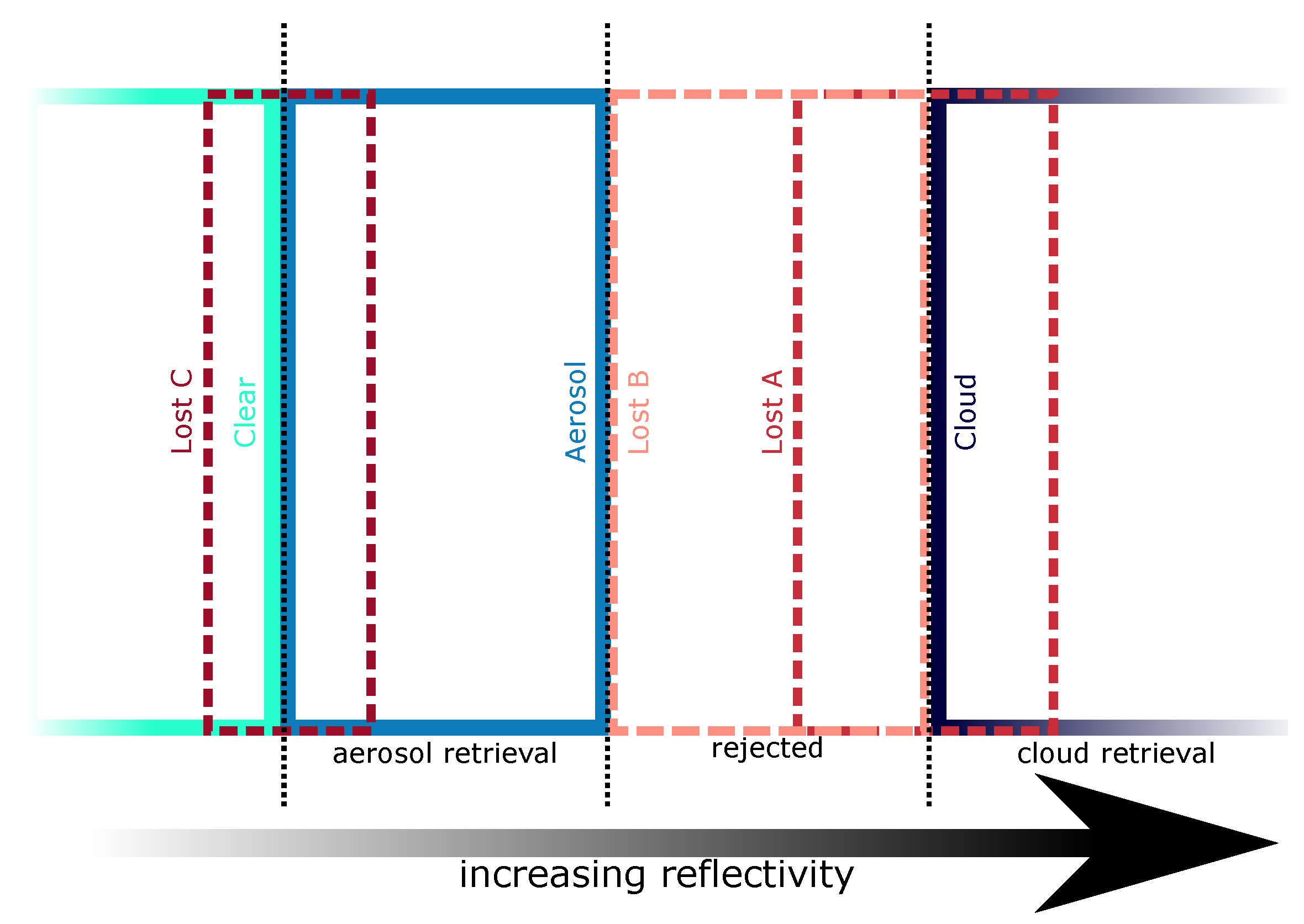
From these considerations, the classes “Lost A”, “Lost B” and “Lost C” can be placed on an aerosol-cloud continuum as shown in
Figure 9.
5. Conclusions
Knowledge about the transition zone between aerosols and clouds was limited so far. Neither cloud nor aerosol property retrievals are performed in this region in order to reduce overall retrieval uncertainties [
6].
The focus of the study was to characterize pixels from MODIS aerosol and cloud products which are neglected by these retrievals, the ”Lost Pixels”. A fifth of the data in all scenes belong to one of the lost classes. The high variability of these pixels allows for a separation of these pixels into the classes “Lost A”, “Lost B” and “Lost C”. The reflective properties of all of these classes are in between cloud and aerosol reflectivities, which indicates that these classes represent a transition zone [
1]. The differences in the distance to the nearest cloud or aerosol pixels based on the ”Lost” classes, as well as the spatial distribution of the frequencies and the mean reflectances, suggest that the class “Lost A” is closer to cloud properties, and the classes “Lost B” and “Lost C” to aerosol properties. “Lost A” pixels are likely cloud fragments, ’Lost B’ hydrated aerosols in between aerosol loaded atmosphere and clouds, and “Lost C” predominantly discarded aerosol pixels from the ACM interpolation (
Figure 9). All of these will require closer attention in the observation-based study of aerosol–cloud interactions, but in particular when evaluating models based on satellite observations.
This study has highlighted not only the extent and properties, but also the spatial distribution of the transition zone between aerosols and clouds, and thus provides an orientation on where and when to look for aerosol-cloud interaction in future research.


