
Remote Sensing Image Registration with Line Segments and Their Intersections


School of Instrumentation Science and Optoelectronics Engineering, Beihang University, No. 37 Xueyuan Road, Beijing 100191, China
*
Author to whom correspondence should be addressed.
Remote Sens. 2017, 9(5), 439; https://doi.org/10.3390/rs9050439
Submission received: 22 March 2017
/
Revised: 26 April 2017
/
Accepted: 30 April 2017
/
Published: 4 May 2017
Abstract
:Image registration is a basic but essential step for remote sensing image processing, and finding stable features in multitemporal images is one of the most considerable challenges in the field. The main shape contours of artificial objects (e.g., roads, buildings, farmlands, and airports) can be generally described as a group of line segments, which are stable features, even in images with evident background changes (e.g., images taken before and after a disaster). In this study, a registration method that uses line segments and their intersections is proposed for multitemporal remote sensing images. First, line segments are extracted in image pyramids to unify the scales of the reference image and the test image. Then, a line descriptor based on the gradient distribution of local areas is constructed, and the segments are matched in image pyramids. Lastly, triplets of intersections of matching lines are selected to estimate affine transformation between two images. Additional corresponding intersections are provided based on the estimated transformation, and an iterative process is adopted to remove outliers. The performance of the proposed method is tested on a variety of optical remote sensing image pairs, including synthetic and real data. Compared with existing methods, our method can provide more accurate registration results, even in images with significant background changes.
1. Introduction
Image registration refers to the process of aligning two images of the same scene taken at different times, from different sensors, or at different views [1,2]. It is the basis of remote sensing image processing, and its result has been widely used in many areas, including image fusion [3], environment monitoring [4], and change detection [5].
Existing image registration methods can be generally divided into two categories: appearance-based methods and feature-based methods. Among appearance-based methods, the most representative approaches are the cross correlation [6] and mutual information [7] methods. These methods directly use the grayscale distribution information of an image in the registration task; they have been extensively used in the area of medical image registration [8]. In feature-based methods, significant features are extracted from images and then matched based on their similarities. These features, which are extracted as shape contours [9], points [10], lines and curves [11], can be more stable than grayscale information. Compared with appearance-based methods, feature-based methods can achieve high-accuracy registration for images with significant differences in grayscale at a lower computation cost. In the area of remote sensing image registration, images are typically taken at different times; thus, difference in grayscale is relatively apparent. Therefore, most existing registration methods for remote sensing images are based on various features.
Among all the features used in image registration, point features are the most common. In 2004, a method called scale-invariant feature transform (SIFT) [12] was proposed; since then, this method has become the most popular point feature descriptor. SIFT extracts local extrema in scale space to achieve scale invariance and then generates descriptors by using local gradient distribution information. To improve robustness or reduce computation cost, various point feature descriptors [13,14,15,16,17,18] have been proposed based on the SIFT descriptor. Bradley [19] proposed a registration method for intensity-range images, where mutual information was combined with SIFT features. Although these SIFT-like features have been widely used in a variety of areas, they continue to exhibit limits in remote sensing images with evident background changes, which affect the location and description of interest points. Therefore, other point features have been proposed in recent years, and shape context (SC) [20] is one of the most well-known; SC uses the points relative to a reference point to generate a descriptor called shape context. Huang and Li [21] first applied shape context to remote sensing image registration. Subsequently, Jiang et al. [22] improved shape context to achieve rotation and scale invariance. However, the performance of these shape context-based methods deteriorates when geometric distortion is caused by a view change between the images. Arandjelović [23] proposed an object matching method using boundary descriptors. The the local curvature maxima along a contour were detected as boundary keypoints. Then, the local boundary descriptor was constructed using the profile of boundary normals’ directions. Finally, the set of boundary descriptors is clustered, and an object is represented. Evaluated on a large data set, this method can successfully match objects in terms of view change. Whereas, since there are abundant objects in a remote sensing image, it might be difficult to represent an object with a cluster of boundary descriptors. The incorrect shape components in remote sensing images may also influence the effectiveness of this method.
Compared with point features, line features in an image contain more geometric and structural information. Thus, registration methods based on line segments have attracted increasing attention in recent years. Existing registration methods based on line segments can be divided into two classes: descriptor-based methods and search-based methods.
In descriptor-based methods, the local appearance of a line segment must be described to match lines with maximal similarity. Bay et al. [24] proposed a line-matching method that used a color histogram to match lines and a topological filter to remove outliers. This method is capable of working with a wide range of scenes based on line segments in color images. Wang et al. [25] proposed a line descriptor called mean-standard deviation line descriptor (MSLD), which was constructed in a SIFT-like manner. MSLD defines the local area of a line segment as a pixel support region (PSR) and then uses the mean and standard deviation of the gradient in PSR to generate a line descriptor. An improved descriptor, called line band descriptor (LBD) [26], was also proposed; it realized scale invariance by using a scale-space line extraction strategy. Verhagen et al. [27] introduced a common method to add scale-invariance to a line descriptor, and scale-invariant MSLD was presented in this manner. Wang et al. [28] clustered line segments into local groups based on their spatial relations. A group of line segments was called a line signature (LS). The similarity of LS features is determined by the length and angle information of line segments, which is sensitive to endpoint changes. Fan et al. [29] introduced a method called line matching leveraged by point correspondences (LP). In this method, an affine invariance from one line and two coplanar points was used to improve the distinctiveness and robustness of line matching. Arandjelović [30] proposed a frontal face recognition algorithm based on edge information. This algorithm can robustly match frontal faces under extreme illuminations; but the vertical symmetry of frontal faces which was used to remove false edges, might not be effective in other scenarios. Shi and Jiang [31] proposed an automatic image registration method that utilized the midpoints of line segments to generate shape context and describe shape contours (named RMLSM for short). The experimental results showed that this method could be used in the registration of remote sensing images with evident background changes. Nonetheless, the location of a midpoint is sensitive to segment fragmentation, which limits the use of this method.
Unlike descriptor-based methods, search-based methods typically use an iterative strategy to register two images without describing line features. Coiras et al. [32] proposed an iterative method for visual-infrared image registration that randomly selected three line segments at a time and used their intersections to calculate the affine matrix between two images. An improved method was presented by Li and Stevenson [33], who adopted a selective search strategy to reduce computation cost. Zhao and Goshtasby [34] introduced a registration method for multitemporal remote sensing images. In this method, four lines in each image are selected concurrently starting from the longest line segment to estimate the homography parameters. Then, the parameters are refined by selecting more lines. This method works efficiently when the scale difference between images is small.
In the present study, a novel registration method for optical remote sensing images is proposed. The method is called registration with line segments and their intersections (or RLI, for short). First, line segments are extracted in the image pyramid. These segments will be used to estimate and unify the scales of the reference image and the test image. The problem of segment fragmentation becomes negligible when the scales of the two images are at close levels. Second, a novel line descriptor is introduced, and the line segments are matched in image pyramids based on the distances of the descriptors. The local area near a line segment remains relatively stable; therefore, this descriptor can obtain a robust description of a line feature. Lastly, a triplet of intersections of matching lines is selected to estimate the affine parameters between images, and the registration result is refined through an iterative process. The experimental results demonstrate that the proposed RLI method can register optical remote sensing images with high accuracy.
2. Methodology
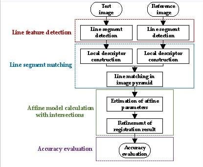
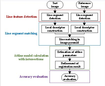
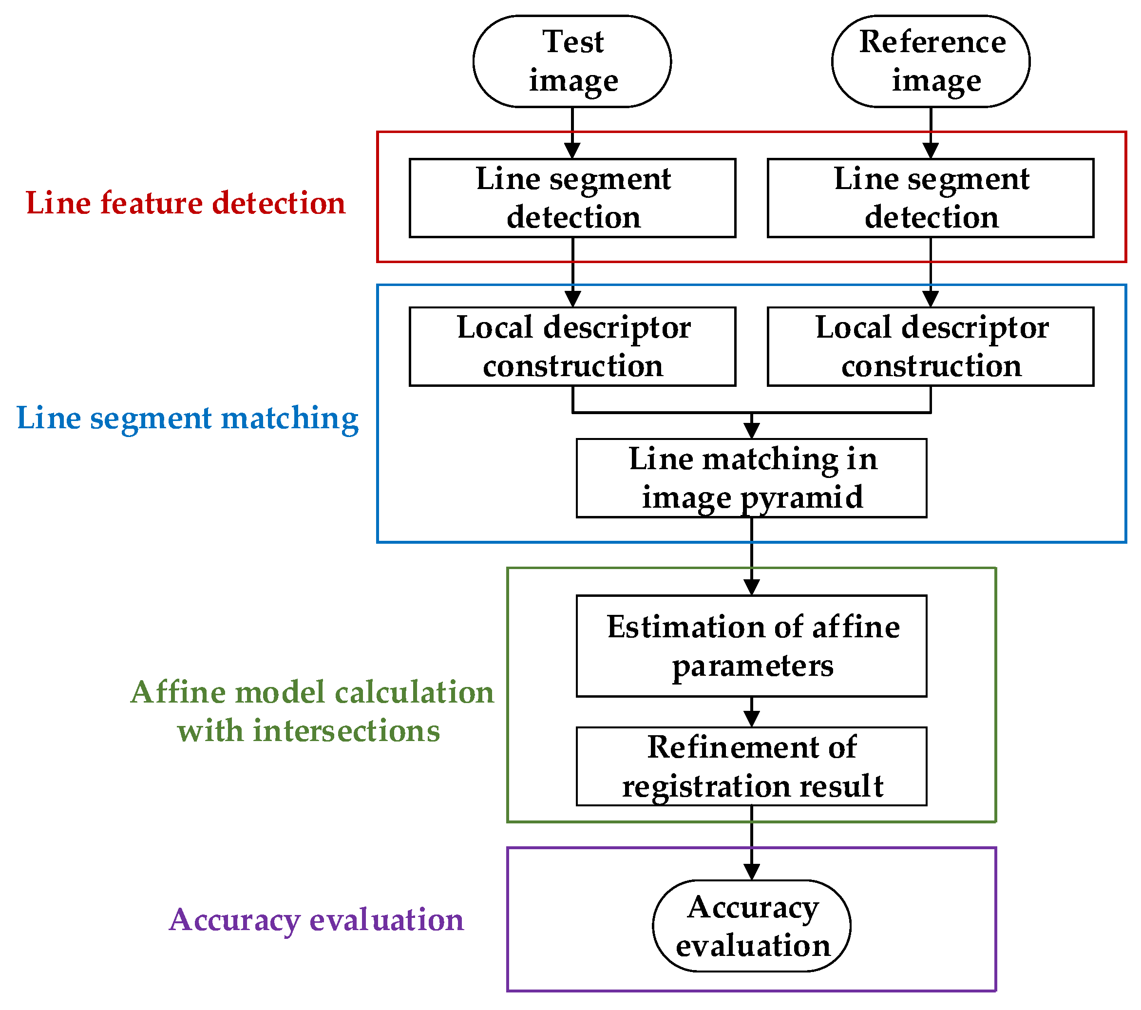
The flowchart of the proposed RLI method is presented in Figure 1. The core steps can be divided into four aspects: line feature detection, line segment matching, affine model calculation with intersections, and accuracy evaluation. These four aspects are described in detail in the succeeding sections.
2.1. Line Segment Detection
Segment fragmentation is a common problem for line detection algorithms, and it has a significant influence on the results of image registration. If the scales of the reference and test images are estimated, then we can unify the scales of these two images via downsampling to overcome the segment fragmentation problem. Thus, we propose a strategy for unifying the scales of images via an image pyramid. First, line segments are extracted from the image pyramid. Second, local descriptors for line segments from different scales are generated. Third, the scales of the two images are estimated by calculating the Euclidean distances of the descriptors. Lastly, the scales of the two images are unified into the same level, and the line segments are matched based on the distances of their descriptors. The image pyramid line segment detection method is presented in this section.
In this study, we assume that all the input images contain a considerable amount of artificial objects (e.g., roads, buildings, farmlands, and airports) that can be detected as line segments. To overcome the problem of segment fragmentation, an image pyramid that consists of n octaves is used. In this image pyramid, each octave is generated by downsampling the original input image with a series of scales, and the first octave is established as the input image. Furthermore, each octave has only one layer; such a scenario differs from the traditional Gaussian pyramid. We can obtain the multi-resolution representation of an image by using this image pyramid.
To detect line segments, EDLines [35] algorithm is used in this paper. EDLines is an automatic line segment detection algorithm with no requirement for parameter tuning, and it is one of the state-of-the-art line detection algorithms [36]. It can obtain meaningful and accurate segments by using a false positive control criterion named the Helmholtz principle [37]. Thus, EDLines is suitable for extracting line segments from the main shape contours in remote sensing images. As shown in Figure 2, EDLines algorithm is applied to each octave image in the image pyramid.
Although EDLines algorithm can obtain meaningful segments as mentioned above, there still exists segment fragmentation in practice. In this study, a line-merging procedure is performed according to the parallel relation and distance of the line segments. The underlying idea of line-merging procedure is to merge two segments that lie on one line belonging to the same shape contour. This procedure can reduce the number of segments by an average of 20%, thereby not only helping improve segment quality but also reduce computation cost. It is worth mentioning that the proposed RLI can work without this line-merging procedure. Then, all the remaining line segments from the ith octave of the pyramid are represented as LineScale[i]. The descriptor for each segment and the image pyramid line matching method are introduced in the following sections.
2.2. Line Segment Matching
In this section, a novel line descriptor based on the distribution of local gradient information is proposed. Unlike descriptors with fixed widths of sub-regions, such as MSLD [25] and LBD [26], the proposed descriptor divides the local area into a series of bands (sub-regions) with gradually changing widths. The center band of this descriptor has the minimal width, and the peripheral bands have the maximal widths. Thus, the widths of bands change gradually, and we called it line descriptor with gradually changing bands (LDGCB). The LDGCB descriptor is more distinctive than traditional descriptors.
2.2.1. Construction of Local Descriptor
Let L denote a line segment with length N in an octave image. Centered on L, a rectangular region, which is also known as the support region, is chosen as the local neighborhood of line segment L. Then, we divide this region into m banded sub-regions , which are parallel with L, and the corresponding widths are . Figure 3 presents an example of the banded sub-regions of line segment L, where and .
Motivated by MSLD, the gradient information is used to determine two critical directions of a line segment. The orthogonal direction is defined as the average gradient orientation of all the pixels on segment L, and the direction is defined as the counterclockwise orthogonal direction of . For each pixel in the rectangular support region, the corresponding gradient g is decomposed into the following two directions , thereby obtaining rotation invariance.
To emphasize the importance of center sub-regions, a Gaussian function with weighting coefficient , is applied to all the rows of the support region, where d is the distance from the row to line L, and is equal to the half width of the entire support region. location changes along direction cause boundary effects; hence, a simple method is provided to reduce these effects. A pixel with gradient g is given in sub-region . Then, g can affect the nearest two sub-regions and , with the weighting coefficients ( and ). We denote the distances from this pixel to the centers of and as and , respectively. We can then obtain the coefficients and .
Let denote the gradient distribution of the jth column in sub-region . The variable is a 4D vector, calculated by accumulating all the gradients in this column along four directions as follows:
where
A description matrix of the gradient distribution, called the band gradient matrix (BGM), is constructed by crossing all columns in sub-region as follows:
The mean and standard deviation of each row in are computed and denoted as two 4D vectors, i.e., and , respectively. After crossing all the BGMs, we obtain a vector with 8m dimensions as follows:
Similar to MSLD, the first half and the second half of LDGCB are normalized separately, thereby guaranteeing that both parts will have equal distinctiveness. A threshold of 0.4 is empirically applied to each element of LDGCB to improve its robustness against nonlinear illumination. Lastly, a renormalization process is performed, and a unit LDGCB descriptor is generated.
2.2.2. Line Segment Matching in Image Pyramids
Line segments and descriptors are generated as discussed in the previous sections. In this section, we present a method to unify the scales of the reference image and the test image, as well as to match line segments at a unified scale. The influence of segment fragmentation is significantly reduced using this method, thereby allowing the registration method to work with a wide range of scale changes. To achieve this goal, the scales of two input images should be first estimated by comparing the Euclidean distances of local descriptors from different octaves of the image pyramid.
Let denote the test image and denote the reference image. These two images of the same scene, are taken at different times, and the ground truth scale between and is denoted as . An image pyramid that consists of N octaves is constructed based on , and the scale between two adjacent octaves is s. The original test image is denoted as , and the ith octave is denoted as . Thus, the scale between and is equal to . The image pyramid based on is constructed in the same manner. In this study, we set and .
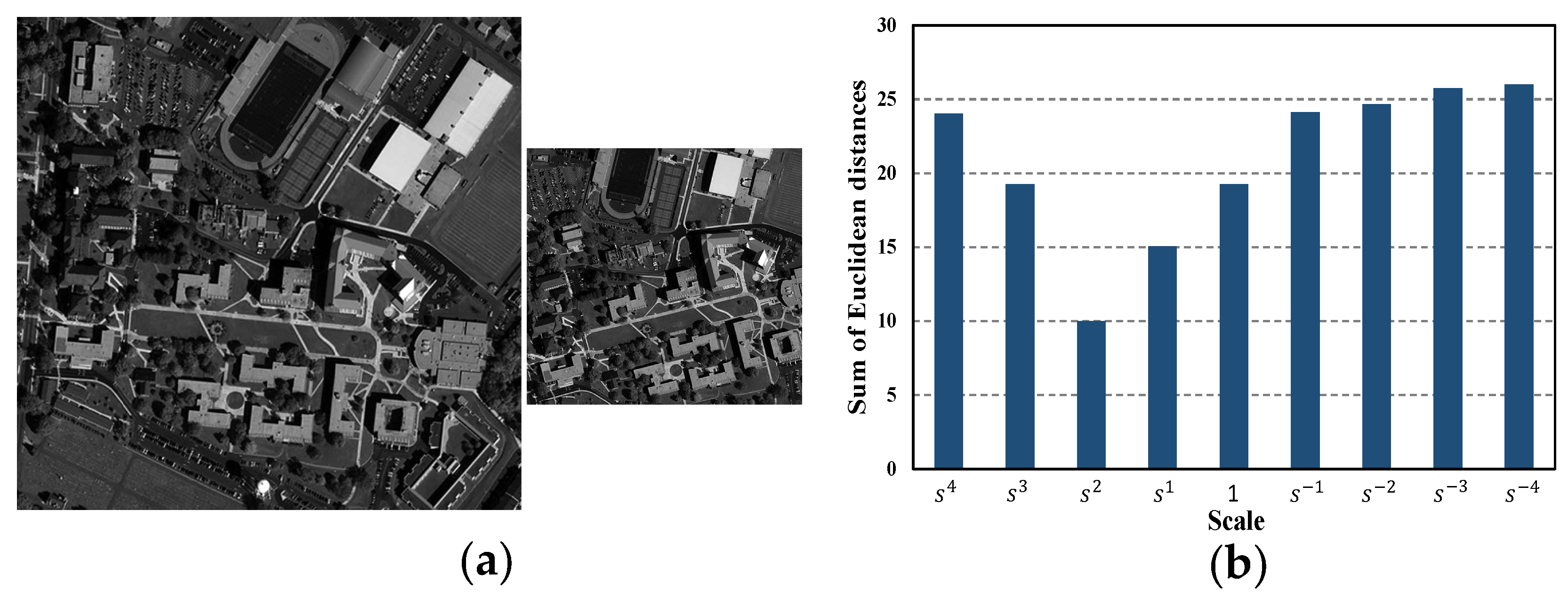
The concept of scale estimation originates from the fact that the distances between tentatively matched descriptors are minimal, when the scales of two images are at the same level. Thus, we can regard the scale with minimal distances as the estimated scale between two images. In this study, descriptors from any octave are tentatively matched with descriptors from the first octave of the other image pyramid. Therefore, candidate scales, i.e., , are observed from the image pyramids. In each candidate scale, the top M least Euclidean distances of the tentatively matched descriptors are accumulated. The scale with the minimal sum of Euclidean distances is denoted as , which is the estimated value of the scale between two images. In this paper, the recommended value range of M is 60 ∼ 120, and we use among all experiments. The qualitative sensitivity analysis of M is given in Section 3.4.3.
An example for scale estimation is provided in Figure 4, where the ground-truth scale between and is . Evidently, the estimated scale is , which is the closest among the nine candidate scales. Furthermore, the sum of the top 100 least distances between tentatively matched descriptors in this estimated scale is significantly smaller than the others, as shown in Figure 4b.
After the scale estimation process, we can unify the scales of the test and reference images by selecting the corresponding octave images. Let and denote the test and reference line segments, respectively, detected from the octave images in the aforementioned estimated scale. Then, these line segments are tentatively matched based on the LDGCB descriptor. Lastly, the candidate matching results are arranged in ascending order of the nearest neighbor distance ratio (NNDR), which is represented as . The matches with low NNDR are more likely to be correct than those with high NNDR.
Compared with close-range images, remote sensing images are sensed from a considerably larger area, and thus, the same type of objects may occur more than once in an image. An effective method to select correct matches is necessary in the area of remote sensing image registration considering the influence of repeated objects. Hence, an iterative process that aims to improve registration accuracy is introduced in the next section.
2.3. Affine Model Calculation with Intersections
Images are sensed remotely with minimal viewpoint changes; hence, the transformation model between two remote sensing images can be approximated to the affine model [38]. The line equations of corresponding lines are generally used to calculate the affine model. However, the intersection points of matching lines have at least two advantages over line equations, namely, lower computation cost and easier outlier removal. Thus, the intersection points of matching lines are selected as tentative matching points in this study, and an iterative process is used to calculate the transformation parameters.
Let T denote the affine model between images. The calculation process for the affine model is divided into two steps: (1) the estimation of affine parameters and (2) the refinement of the registration result. In Step (1), the affine model is estimated iteratively using three intersection pairs at a time, and the final estimated model is denoted as . In Step (2), additional intersections are provided as candidate matching points, thereby refining the affine model . Before these two steps, an intuitive and effective similarity metric is addressed.
2.3.1. Similarity Metric
The number of matched pixels (NMP) is proposed as a similarity metric in [39]; that is, it indicates the number of matched pixels between two edge images transformed via affine transformation T. NMP is an intuitionistic reflection of the similarity between images, and a high value of NMP suggests a good estimated value of T. Nevertheless, this similarity metric frequently fails in the field of remote sensing image registration, in which the high resolution of images typically leads to considerable difficulty in matching pixels directly.
To adapt to high-resolution remote sensing images, an improvement to NMP called score of nearest pixels (SNP) is proposed. The implementation of SNP is as follows. A pixel is given in the test edge image, and is transformed into by affine model . Then, the nearest point of is identified as in the reference edge image, and the distance between and is denoted as . The SNP of is computed as follows:
where the maximal sensitive distance is three pixels. The final SNP is determined by crossing all the pixels in the test edge image as follows:
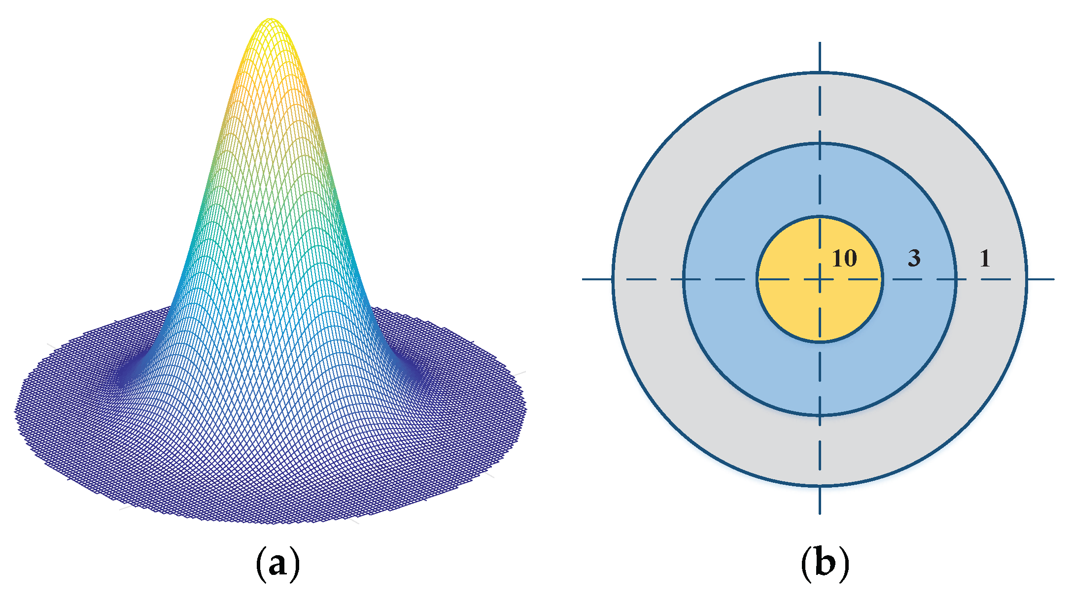
The idea of parameter settings of SNP metric comes from 2D Gaussian distribution model, as shown in Figure 5. Given 2D Gaussian distribution
where is equal to one pixel, about 68% of values are within one pixel; about 95% of the values are within two pixels; and about 99.7% are within 3 pixels [40]. Then, taking the probabilities of different distances as weights, the parameters of SNP are set to integers for calculating easily. This scoring model (as shown in Figure 5b) not only emphasizes the importance of matched pixels (within one pixel), but also extends the sensitivity range to three pixels. Thus, the proposed SNP metric can sufficiently describe similarity in high-resolution images by scoring the nearest edge pixels based on their distance.
In order to reduce the computation cost of calculating the similarity metric, the distance transform [41] is used. In this paper, the distance transform is applied to the reference edge image. The result is a grayscale image, in which each pixel is assigned to the distance of its nearest edge pixel. Distance transform is computed only once for each image pair to be registered, thereby reducing the computation cost efficiently.
2.3.2. Estimation of Affine Parameters
As mentioned in Section 2.2.2, the tentatively matched lines with low NNDR are more likely to be correct than those with high NNDR. Therefore, a new set of candidate matches with NNDR less than 0.75, is empirically selected from and denoted as .
An iterative process is adopted to estimate the affine model between images. In each iteration, a triplet of matching line segments is selected from , and the affine parameters are determined based on their intersections. All the intersections must be located in a rectangular region around the image with an area that is three times larger than the image area. If this location constraint is not satisfied, then this iteration is skipped.
Figure 6 illustrates the process where triplets of intersections are generated from matching lines . At first, a triplet match is chosen to generate intersections. Since the intersection of and does not satisfy the location constraint (colored red in Figure 6b), this iteration is skipped. Then, is selected, and all the three corresponding intersections satisfy the location constraint. This triplet of intersections is used to estimate the affine parameters. Another feasible triple match is in this example. The location constraint in this paper is effective, because intersections not satisfying the location constraint often come from low-quality line pairs with long distances (such as and ) or close directions (such as and ).
An updating strategy of SNP is used in the iterative process, and its implementation is described as follows. The current maximal value of SNP is denoted as MAXSNP. If SNP is greater than MAXSNP in an iteration, then we update the value of MAXSNP and the estimated affine model . After the iteration, the affine model between two images is estimated as . In the ideal situation, the estimated affine model , which is determined from a single triplet of matching line segments, can be regarded as the final affine model. In reality, however, many line segments in can be utilized to improve the accuracy of registration. Therefore, additional corresponding segments are provided to refine the affine transformation in the succeeding section.
2.3.3. Refinement of Registration Result
In this section, additional corresponding intersections are provided to the candidate matching points based on the estimated affine model . Subsequently, is refined by removing the outliers.
To determine which intersection pair can be added as a candidate match, a simple method is introduced in this study. First, each two corresponding lines of intersect at , and the projected distance of this point pair is calculated as . Second, the intersection pairs with projected distances greater than four pixels are removed. Lastly, all the remaining point pairs are arranged in ascending order of the projected distance, and the top 100 point pairs are stored as candidate matching points, i.e., , where .
The affine parameters are refined iteratively based on the SNP similarity metric, and the least squares method is used to calculate the affine model in each iteration. In each iteration, we remove the point pair (starting from the point pair with the maximum projected distance) if the similarity metric is improved without this point pair, and then update the affine parameters and SNP metric. The iteration is terminated when the similarity metric is no longer updated.
After the iteration, all the preserved point pairs are stored in a set of matching points , and the final affine model is calculated from using the least squares method.
2.4. Accuracy Evaluation
To evaluate the performance of the proposed RLI method, three types of criteria are used in this study, namely, number of correct matches, precision, and root-mean-square error (RMSE), which are expressed as follows:
The refers to the number of correct matches in the final matching results, whereas refers to the number of false matches in the final matching results. The image pairs are first registered by an expert, and then the ground truth affine models are generated. A point pair is considered a correct match when its projected distance is less than three pixels.
3. Experiment and Results
In this section, the performance of the proposed RLI method is evaluated on a series of synthetic and real remote sensing image pairs, and then compared with the performances of RMLSM [31], SIFT [12], MSLD [25] and LP [29]. The parameter setting, data sets, and experimental results are presented as follows.
3.1. Parameter Setting
The VLFeat [42] implementation of SIFT is adopted is this study, and the threshold of the matching criterion NNDR is set to 0.6. The implementation of RMLSM, MSLD and LP is based on the source codes of the original authors. The EDLines [35] algorithm is used to detect line segments with the default parameters.
In the proposed LDGCB descriptor, two parameters, namely, the number of sub-regions m and their widths , are used. These parameters are selected based on an experiment on seven image pairs. The total number of correct matches and the dimension of the descriptor are provided in Table 1. The ideal parameter leads to a considerable number of correct matches with low descriptor dimensions. In this study, we set , , which results in a 72-dimensional descriptor. It is worth mentioning that there might be better parameters of descriptors and the current choice of these parameters can be seen a trade-off between performance and time cost.
3.2. Data Sets
The test data sets are composed of two types of images, i.e., synthetic and real multitemporal remote sensing images, with a ground sample distance (GSD) ranging from 0.5 m to 231.65 m, and their characteristics are provided in Table 2. The examples of synthetic images are shown in Figure 7, and the real image pairs are shown in Figure 8.
To test robustness on the aspects of scale, rotation, illumination and cloud cover, a series of synthetic images are generated from Data set 1-1. Each type of challenging condition is composed of six synthetic images and an original image. Figure 7 shows several examples of the synthetic images.
3.3. Experimental Results
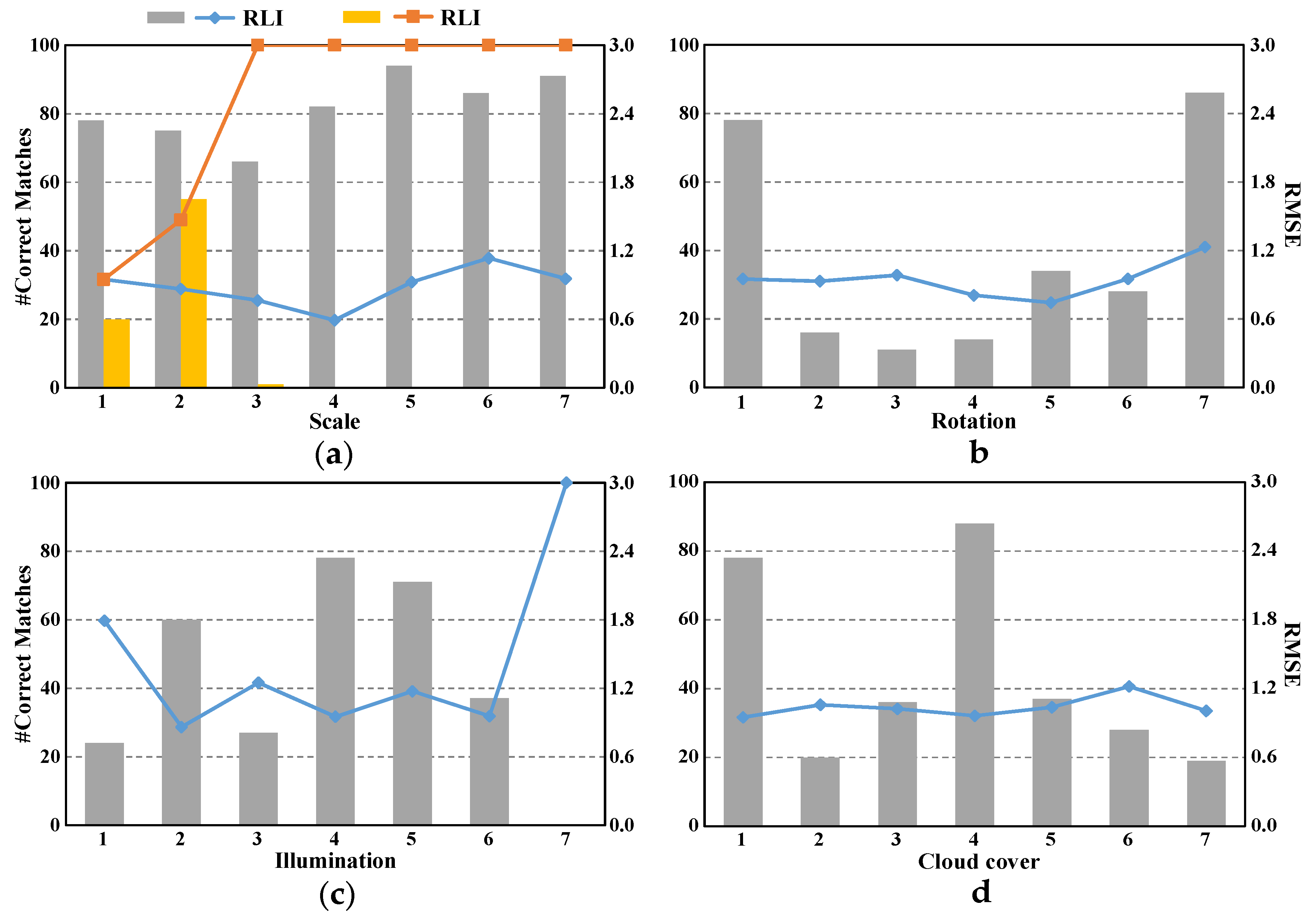
In this study, the EDLines algorithm is used to detect line segments in an image pyramid. Then, the proposed LDGCB descriptor is constructed, and the lines are tentatively matched in a unified scale. Lastly, the intersections of matching lines are used to estimate and refine the affine model. Figure 9 shows the experimental results of the synthetic images in terms of RMSE and number of correct matches.
Figure 9a presents the performances of RLI and RLI without an image pyramid (marked as RLI-S). From image No. 1 to No. 7, the scale ratio between the synthetic image and the original image varies from 1.0 to 0.4. As expected, the image pyramid improves robustness against scale changes. In practice, if the scale ratio between two images are known to be close to 1 (as prior knowledge), the RLI method can work without image pyramids. Figure 9b shows the results of the images with rotation angles varying from 0 to . RMSE remains stable in this test, and the number of correct matches performs well when the rotation angle is 0 or , where no aliasing of the line segments occurs. Figure 9c shows the performance against image illumination changes. To evaluate this effect, we transfer the original image into HSV color space [43] and then change the value to simulate illumination changes. The simulated illumination varies from half to twice the original illumination. The results show that the proposed method is relatively robust to illumination changes within a certain range. Figure 9d illustrates the effect of cloud cover. Six synthetic images are generated by adding randomly distributed patches of clouds, and the number of patches varies from 60 to 360. The proposed method can accurately register images with a mass of clouds given the effectiveness of the local descriptor.
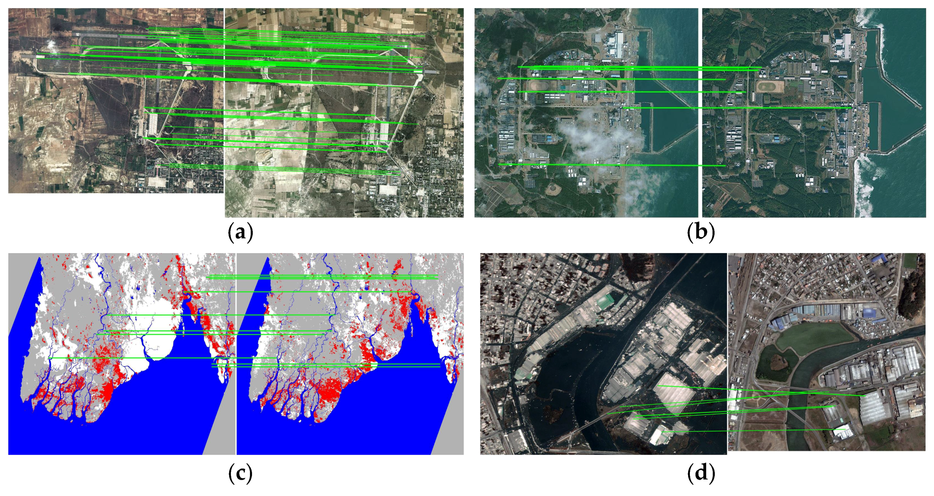
Table 3 shows the comparative experimental results of RLI and four other algorithms on real remote sensing image pairs, with respect to the number of correct matches, precision, and RMSE. As for RLI, the projected distances of corresponding intersections are shown in Table 4. The matching intersection points of the proposed RLI method are shown in Figure 10.
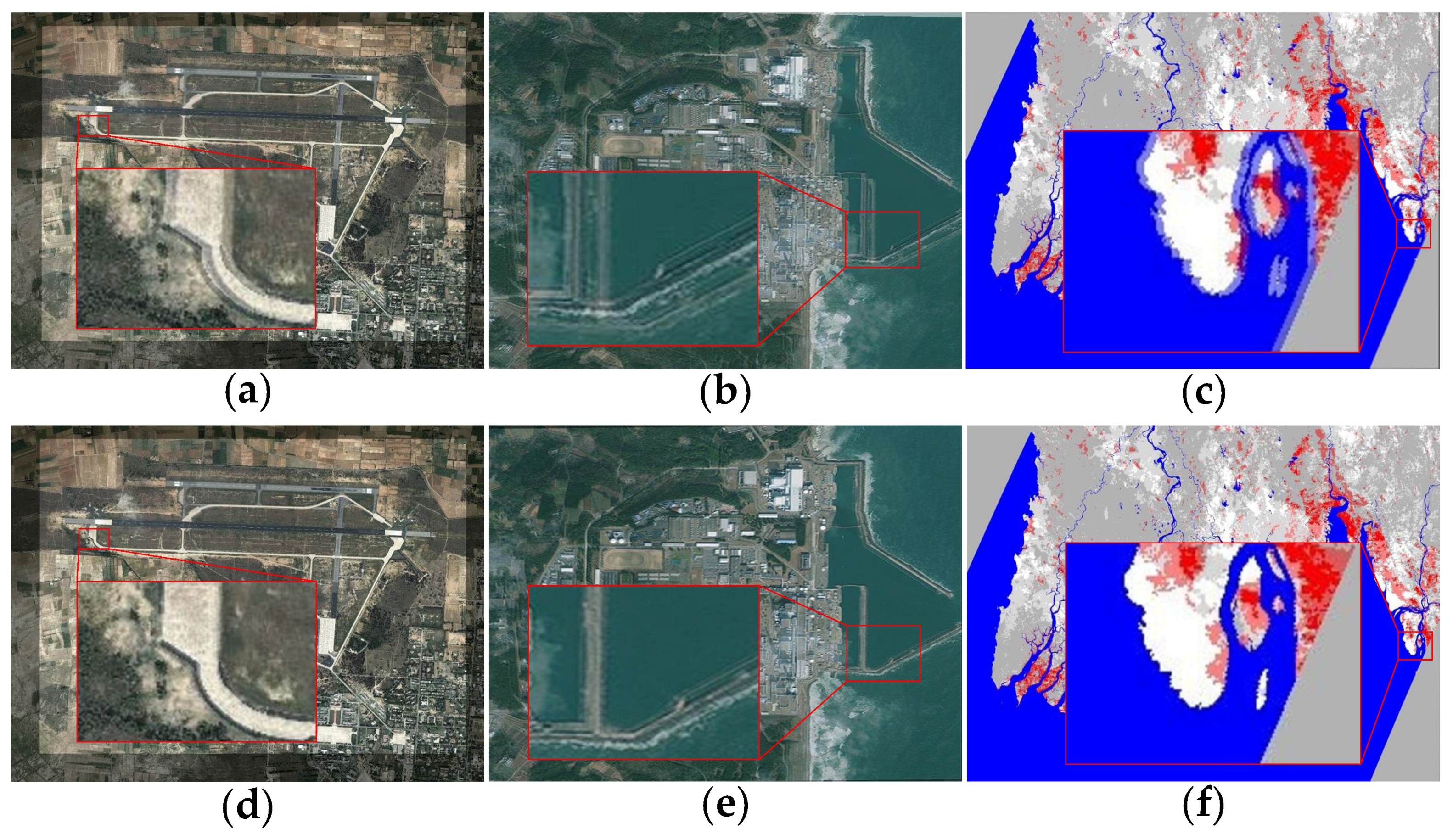
Figure 11 shows the registration results (fusion images of test and reference images) for three real image pairs, in which Figure 11a corresponds to MSLD on Data set 2-1, Figure 11b corresponds to SIFT on Data set 2-2, Figure 11c corresponds to LP on Data set 2-3, and Figure 11d–f correspond to RLI on these three data sets. For each registration result, a sub-region of the fusion image is enlarged for visual assessment. The enlarged sub-region explicitly shows the registration result on the main shapes of objects, such as roads and coastlines. Evidently, the proposed RLI method can align the main shapes in the images with high accuracy.
3.4. Sensitivity Analysis
3.4.1. Types of Images
In general, the performance of a registration method is greatly effected by the types of test and reference images. In this paper, the intersections of matching lines are used to calculate the affine parameters between two images. Intersections are meaningful and effective when the line segments come from coplanar objects even in images with significant background changes, which has been confirmed by the experiments.
However, if there is significant displacement of the scene in images, it is difficult to register those images by applying rigid transformation model like affine function. Rather, non-rigid model such as piecewise linear function [44,45] is suitable. Moreover, the intersections of non-coplanar lines are meaningless and cannot be used to register images with displacement of the scene. Thus, in this paper, we focus on the registration of satellite remote sensing images, where the affine model is suitable.
3.4.2. Parameters of Local Descriptor
The performance of local descriptor determines the number of corresponding lines. Generally speaking, more corresponding lines can lead to a better registration result. In the proposed LDGCB descriptor, two parameters, namely, the number of sub-regions m and their widths , are used. These parameters are selected based on an experiment as shown in Table 1. In this study, we set , , which results in a 72-dimensional descriptor. This choice is good, and the current descriptor can obtain abundant correct matches in remote sensing images. Moreover, since the space of possible choices of parameters is really large, and there might be better choices of these parameters.
3.4.3. Parameters of Scale Estimation
In order to improve the robustness against scale changes, the scale ratio between two images is estimated using image pyramids. The scale with minimal difference between descriptors is treated as the closest scale. Thus, the sum of top M least distances of tentatively matching descriptors is chosen for scale estimation. If M is too small, the scale estimation is easily effected by stochastic factors. If it is too large, the sum of descriptors can be less discriminative because of the influence of incorrect matches. In practice, since the performances of a descriptor varies significantly in different scales, the scale estimation can be carried out in a wide range of M. In this paper, the recommended value range of M is 60 ∼ 120, and we use among all experiments.
3.4.4. Parameters of Similarity Metric
The parameters of the proposed SNP similarity metric are motivated by 2D Gaussian distribution model (shown in Figure 5). For a 2D Gaussian distribution, the three-sigma rule [40] expresses a conventional heuristic that “nearly all” values (99.7%) are within three standard deviations of the mean. In this paper, we extend the traditional NMP (number of matched pixels) metric [39] to SNP (score of nearest pixels). The sensitive distance of SNP is set to three pixels, which is treated as a three-sigma area. Then, taking the probabilities of different distances as weights, the parameters of SNP are set to integers for calculating easily. This scoring model not only emphasizes the importance of matched pixels (within one pixel), but also extends the sensitivity range to three pixels. In practice, the extension of sensitive range makes the metric more suitable for large-size images, and a narrow sensitive range is more suitable for small-size images.
4. Discussion
A novel registration method for multitemporal optical remote sensing images based on line segments and their intersections is proposed in this study. The performance of RLI is investigated through a variety of experiments on synthetic and real remote sensing images, and the qualitative sensitivity analysis is given in this paper.
The validity of image pyramid line segment detection is proven using the first group of synthetic images. The RLI method achieves robustness against scale changes by unifying the scales of images. All the experimental results on synthetic images shows that RLI is robust to scale, rotation, illumination, and cloud cover, thereby indicating that RLI can be used to register images with evident background changes (e.g., images taken before and after a disaster).
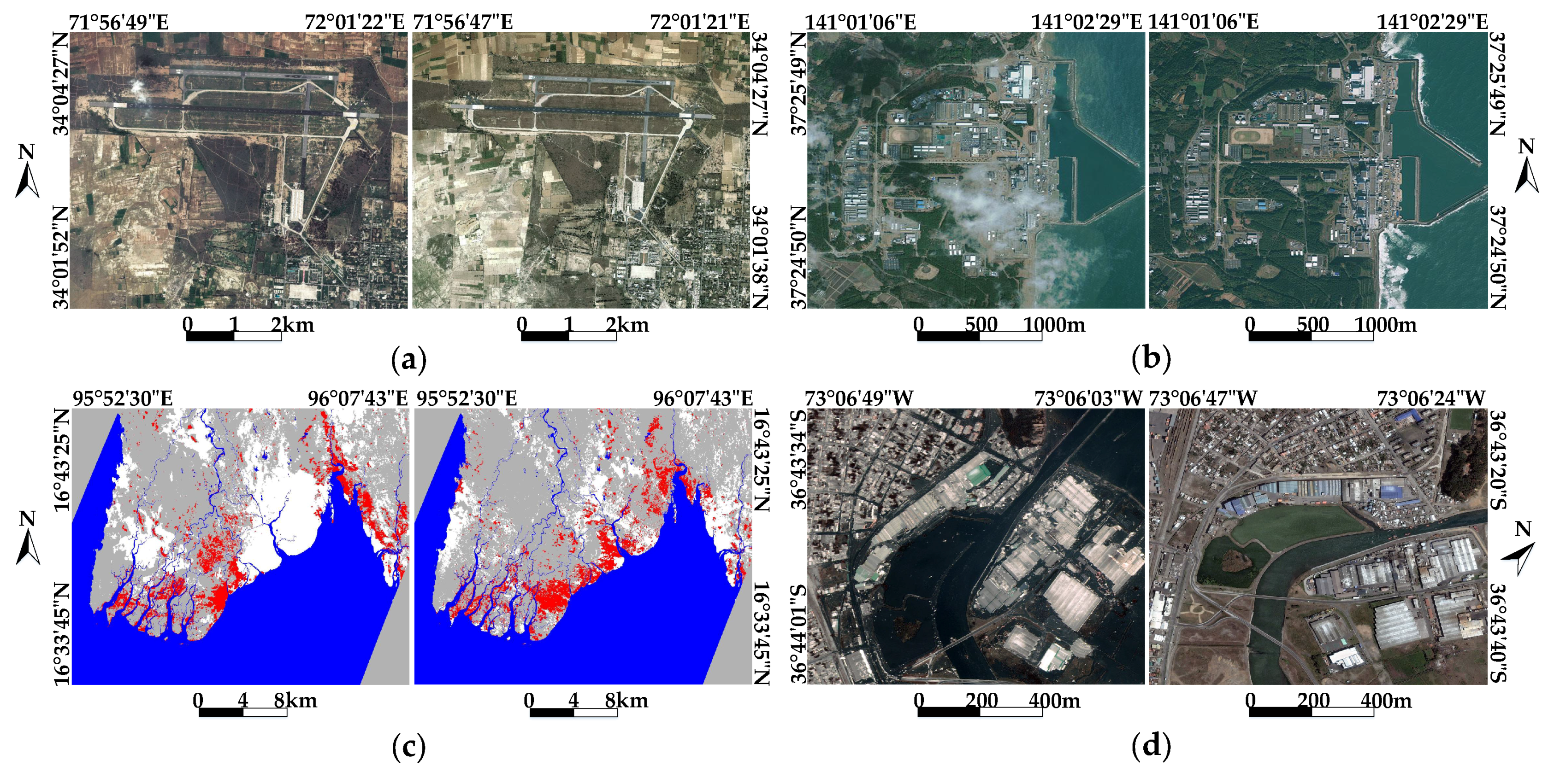
In this study, real remote sensing image pairs present considerable challenges to a registration method, and their characteristics are as follows. The high-resolution images (with 2 m GSD) in Data set 2-1 are taken by QuickBird at different times, and the background is influenced by floods in Pakistan. The runways in the airport are preserved completely, which can be detected as line features. The images in Data set 2-2 are taken by SPOT4 before and after a tsunami, and they are medium-resolution images (with 10 m GSD). Certain objects in this image pair are damaged by the tsunami. Furthermore, excessive cloud cover is present in this data set. Data set 2-3 corresponds to the MODIS Flood Maps from Aqua satellites. This data set is composed of low-resolution images (with 231.65 m GSD) before and after the Myanmar floods. The flooded regions are shown in red, the original water regions are shown in blue, land is gray, and clouds are white. Although the background changes considerably in this data set, the main shapes of the objects remain stable. Data set 2-4 are high-resolution remote sensing images (with 0.61 m GSD) taken by QuickBird. There are significant geometric distortions and background changes in this data set. This data set is the most challenging one among all the four real data sets.
As shown in Table 3, RLI outperforms other methods on these challenging real data sets. RMLSM performs the second best among all methods. However, influenced by the geometric distortions, its precision decreases on Data set 2-4. The average RMSE of RLI on real image pairs is 0.90, whereas those for RMLSM, MSLD, SIFT, and LP are 1.08, 1.23, 1.26 and 1.22, respectively. Furthermore, the precision of RLI remains at on all the data sets, thereby indicating that all the output matches are correct correspondences.
The main reasons for the good performance of RLI are analyzed as follows. (1) When faced with background changes in images, the main shape contours of artificial objects are more stable than point features; these shape contours can be extracted as a group of line segments; (2) The proposed local descriptor is more distinctive and detailed than MSLD; (3) The RLI method can register images with high accuracy by using the intersection points of matching lines to estimate and refine the affine parameters through an iterative process. In practice, our method can also be used to register general images with coplanar lines under affine transformation.
In this study, the use of an iterative strategy for result refinement improves the accuracy of the registration results. However, this process leads to a rapid increase in computation cost when an image is large. Our next work will focus on improving the speed of image registration under the precondition of high accuracy.
5. Conclusions
A registration method based on line segments and their intersections has been proposed for optical remote sensing images in this study. First, the EDLines algorithm is used to detect line segments. To improve robustness against scale changes, the scales of the test image and the reference image are unified into the same level with the use of image pyramids. Then, a novel line descriptor is introduced based on the local gradient information of a line segment, and line segments are matched according to the distances of descriptors. Lastly, triplets of intersection points of matching lines are selected to estimate affine parameters, and the registration result is refined through an iterative process. The experimental results of the synthetic image pairs show that the RLI method is robust to scale, rotation, illumination, and cloud cover. Four challenging real image pairs are selected to analyze the performance of RLI, and the results indicate that RLI outperforms four other methods in terms of RMSE and precision.
In this study, the problem of line-based registration is solved by combining line segments and their intersection points. The stability of line features and the validity of calculating affine transformation via intersection points have been proven by the experimental results, even in images with significant background changes.
In the future, a more robust line segment detector, which can extract complete line segments in disaster images, should be investigated. In addition, the computation speed of the proposed registration method should be improved.
Acknowledgments
The authors would like to thank the anonymous reviewers and editors for their profound comments. This research is supported by the National Natural Science Foundation of China (No. 61222304) and Specialized Research Fund for the Doctoral Program of Higher Education (No. 20121102110032). We also acknowledge the help of China Earthquake Disaster Prevention Center for providing part of the experimental datasets.
Author Contributions
Chengjin Lyu conceived the experiments and wrote the paper. Jie Jiang supervised the study and reviewed the manuscript.
Conflicts of Interest
The authors declare no conflict of interest.
References
- Zitova, B.; Flusser, J. Image registration methods: A survey. Image Vis. Comput. 2003, 21, 977–1000. [Google Scholar] [CrossRef]
- Dawn, S.; Saxena, V.; Sharma, B. Remote sensing image registration techniques: A survey. In Proceedings of the 4th International Conference on Image and Signal Processing (ICISP), Trois-Rivières, QC, Canada, 30 June–2 July 2010; pp. 103–112. [Google Scholar]
- Ehlers, M. Multisensor image fusion techniques in remote sensing. ISPRS J. Photogramm. Remote Sens. 1991, 46, 19–30. [Google Scholar] [CrossRef]
- Moskal, L.M.; Styers, D.M.; Halabisky, M. Monitoring Urban Tree Cover Using Object-Based Image Analysis and Public Domain Remotely Sensed Data. Remote Sens. 2011, 3, 2243–2262. [Google Scholar] [CrossRef]
- Alberga, V. Similarity Measures of Remotely Sensed Multi-Sensor Images for Change Detection Applications. Remote Sens. 2009, 1, 122–143. [Google Scholar] [CrossRef]
- Debella-Gilo, M.; Kääb, A. Sub-pixel precision image matching for measuring surface displacements on mass movements using normalized cross-correlation. Remote Sens. Environ. 2011, 115, 130–142. [Google Scholar] [CrossRef]
- Maes, F.; Collignon, A.; Vandermeulen, D.; Marchal, G.; Suetens, P. Multimodality image registration by maximization of mutual information. IEEE Trans. Med. Imaging 1997, 16, 187–198. [Google Scholar] [CrossRef] [PubMed]
- Hill, D.L.; Batchelor, P.G.; Holden, M.; Hawkes, D.J. Medical image registration. Phys. Med. Biol. 2001, 46, R1. [Google Scholar] [CrossRef] [PubMed]
- Jiang, J.; Cao, S.; Zhang, G.; Yuan, Y. Shape registration for remote-sensing images with background variation. Int. J. Remote Sens. 2013, 34, 5265–5281. [Google Scholar] [CrossRef]
- Wang, C.Y.; Sun, H.; Yada, S.; Rosenfeld, A. Some experiments in relaxation image matching using corner features. Pattern Recognit. 1983, 16, 167–182. [Google Scholar] [CrossRef]
- Schmid, C.; Zisserman, A. The geometry and matching of lines and curves over multiple views. Int. J. Comput. Vis. 2000, 40, 199–233. [Google Scholar] [CrossRef]
- Lowe, D.G. Distinctive image features from scale-invariant keypoints. Int. J. Comput. Vis. 2004, 60, 91–110. [Google Scholar] [CrossRef]
- Ke, Y.; Sukthankar, R. PCA-SIFT: A more distinctive representation for local image descriptors. In Proceedings of the IEEE Conference on Computer Vision and Pattern Recognition (CVPR), Washington, DC, USA, 27 June–2 July 2004. [Google Scholar]
- Bay, H.; Ess, A.; Tuytelaars, T.; Van Gool, L. Speeded-up robust features (SURF). Comput. Vis. Image Underst. 2008, 110, 346–359. [Google Scholar] [CrossRef]
- Morel, J.M.; Yu, G. ASIFT: A new framework for fully affine invariant image comparison. SIAM J. Imaging Sci. 2009, 2, 438–469. [Google Scholar] [CrossRef]
- Rublee, E.; Rabaud, V.; Konolige, K.; Bradski, G. ORB: An efficient alternative to SIFT or SURF. In Proceedings of the IEEE International Conference on Computer Vision (ICCV), Florence, Italy, 2011; pp. 2564–2571. [Google Scholar]
- Sedaghat, A.; Mokhtarzade, M.; Ebadi, H. Uniform robust scale-invariant feature matching for optical remote sensing images. IEEE Trans. Geosci. Remote Sens. 2011, 49, 4516–4527. [Google Scholar] [CrossRef]
- Dellinger, F.; Delon, J.; Gousseau, Y.; Michel, J.; Tupin, F. SAR-SIFT: A SIFT-like algorithm for SAR images. IEEE Trans. Geosci. Remote Sens. 2015, 53, 453–466. [Google Scholar] [CrossRef]
- Bradley, P.E.; Jutzi, B. Improved Feature Detection in Fused Intensity-Range Images with Complex SIFT (ℂSIFT). Remote Sens. 2011, 3, 2076–2088. [Google Scholar] [CrossRef]
- Belongie, S.; Malik, J.; Puzicha, J. Shape matching and object recognition using shape contexts. IEEE Trans. Pattern Anal. Mach. Intell. 2002, 24, 509–522. [Google Scholar] [CrossRef]
- Huang, L.; Li, Z. Feature-based image registration using the shape context. Int. J. Remote Sens. 2010, 31, 2169–2177. [Google Scholar] [CrossRef]
- Jiang, J.; Zhang, S.; Cao, S. Rotation and scale invariant shape context registration for remote sensing images with background variations. J. Appl. Remote Sens. 2015, 9, 095092. [Google Scholar] [CrossRef]
- Arandjelović, O. Object matching using boundary descriptors. In Proceedings of the British Machine Vision Association Conference (BMVC), Guildford, UK, 3–7 September 2012; pp. 1–11. [Google Scholar]
- Bay, H.; Ferraris, V.; Van Gool, L. Wide-baseline stereo matching with line segments. In Proceedings of the IEEE Computer Society Conference on Computer Vision and Pattern Recognition (CVPR), San Diego, CA, USA, 20–25 June 2005; Volume 1, pp. 329–336. [Google Scholar]
- Wang, Z.; Wu, F.; Hu, Z. MSLD: A robust descriptor for line matching. Pattern Recognit. 2009, 42, 941–953. [Google Scholar] [CrossRef]
- Zhang, L.; Koch, R. An efficient and robust line segment matching approach based on LBD descriptor and pairwise geometric consistency. J. Vis. Commun. Image Represent. 2013, 24, 794–805. [Google Scholar] [CrossRef]
- Verhagen, B.; Timofte, R.; Van Gool, L. Scale-invariant line descriptors for wide baseline matching. In Proceedings of the IEEE Winter Conference on Applications of Computer Vision (WACV), Steamboat Springs, CO, USA, 24–26 March 2014; pp. 493–500. [Google Scholar]
- Wang, L.; Neumann, U.; You, S. Wide-baseline image matching using line signatures. In Proceedings of the IEEE International Conference on Computer Vision (ICCV), Kyoto, Japan, 29 September–2 October 2009; pp. 1311–1318. [Google Scholar]
- Fan, B.; Wu, F.; Hu, Z. Line matching leveraged by point correspondences. In Proceedings of the IEEE Conference on Computer Vision and Pattern Recognition (CVPR), San Francisco, CA, USA, 15–17 June 2010; pp. 390–397. [Google Scholar]
- Arandjelović, O. Gradient edge map features for frontal face recognition under extreme illumination changes. In Proceedings of the British Machine Vision Association Conference (BMVC), Guildford, UK, 3–7 September 2012; pp. 1–11. [Google Scholar]
- Shi, X.; Jiang, J. Automatic Registration Method for Optical Remote Sensing Images with Large Background Variations Using Line Segments. Remote Sens. 2016, 8, 426. [Google Scholar] [CrossRef]
- Coiras, E.; Santamarı, J.; Miravet, C. Segment-based registration technique for visual-infrared images. Opt. Eng. 2000, 39, 282–289. [Google Scholar] [CrossRef]
- Li, Y.; Stevenson, R.L. Multimodal Image Registration with Line Segments by Selective Search. IEEE Trans. Cybern. 2016, 47, 1–14. [Google Scholar] [CrossRef] [PubMed]
- Zhao, C.; Goshtasby, A.A. Registration of multitemporal aerial optical images using line features. ISPRS J. Photogramm. Remote Sens. 2016, 117, 149–160. [Google Scholar] [CrossRef]
- Akinlar, C.; Topal, C. EDLines: A real-time line segment detector with a false detection control. Pattern Recognit. Lett. 2011, 32, 1633–1642. [Google Scholar] [CrossRef]
- Yang, X.; Qin, X.; Wang, J.; Wang, J.; Ye, X.; Qin, Q. Building Façade Recognition Using Oblique Aerial Images. Remote Sens. 2015, 7, 10562–10588. [Google Scholar] [CrossRef]
- Desolneux, A.; Moisan, L.; Morel, J.M. Meaningful alignments. Int. J. Comput. Vis. 2000, 40, 7–23. [Google Scholar] [CrossRef]
- Flusser, J.; Suk, T. A moment-based approach to registration of images with affine geometric distortion. IEEE Trans. Geosci. Remote Sens. 1994, 32, 382–387. [Google Scholar] [CrossRef]
- Simonson, K.M.; Drescher, S.M.; Tanner, F.R. A statistics-based approach to binary image registration with uncertainty analysis. IEEE Trans. Pattern Anal. Mach. Intell. 2007, 29, 112–125. [Google Scholar] [CrossRef] [PubMed]
- Pukelsheim, F. The three sigma rule. Am. Stat. 1994, 48, 88–91. [Google Scholar] [CrossRef]
- Arandjelović, O. Colour invariants under a non-linear photometric camera model and their application to face recognition from video. Pattern Recognit. 2012, 45, 2499–2509. [Google Scholar] [CrossRef]
- Vedaldi, A.; Fulkerson, B. VLFeat: An open and portable library of computer vision algorithms. In Proceedings of the 18th ACM International Conference on Multimedia, Firenze, Italy, 25–29 October 2010; pp. 1469–1472. [Google Scholar]
- Smith, A.R. Color gamut transform pairs. ACM Comput. Graph. 1978, 12, 12–19. [Google Scholar] [CrossRef]
- Goshtasby, A. Piecewise linear mapping functions for image registration. Pattern Recognit. 1986, 19, 459–466. [Google Scholar] [CrossRef]
- Han, Y.; Choi, J.; Byun, Y.; Kim, Y. Parameter optimization for the extraction of matching points between high-resolution multisensor images in urban areas. IEEE Trans. Geosci. Remote Sens. 2014, 52, 5612–5621. [Google Scholar]
Figure 1.
Flowchart of the proposed method.

Figure 2.
Illustration of line segment detection in an image pyramid. The first octave is the input image, and the other octave images are downsampled from it. Line segments detected from the ith octave image are represented as LineScale[i].
Figure 2.
Illustration of line segment detection in an image pyramid. The first octave is the input image, and the other octave images are downsampled from it. Line segments detected from the ith octave image are represented as LineScale[i].
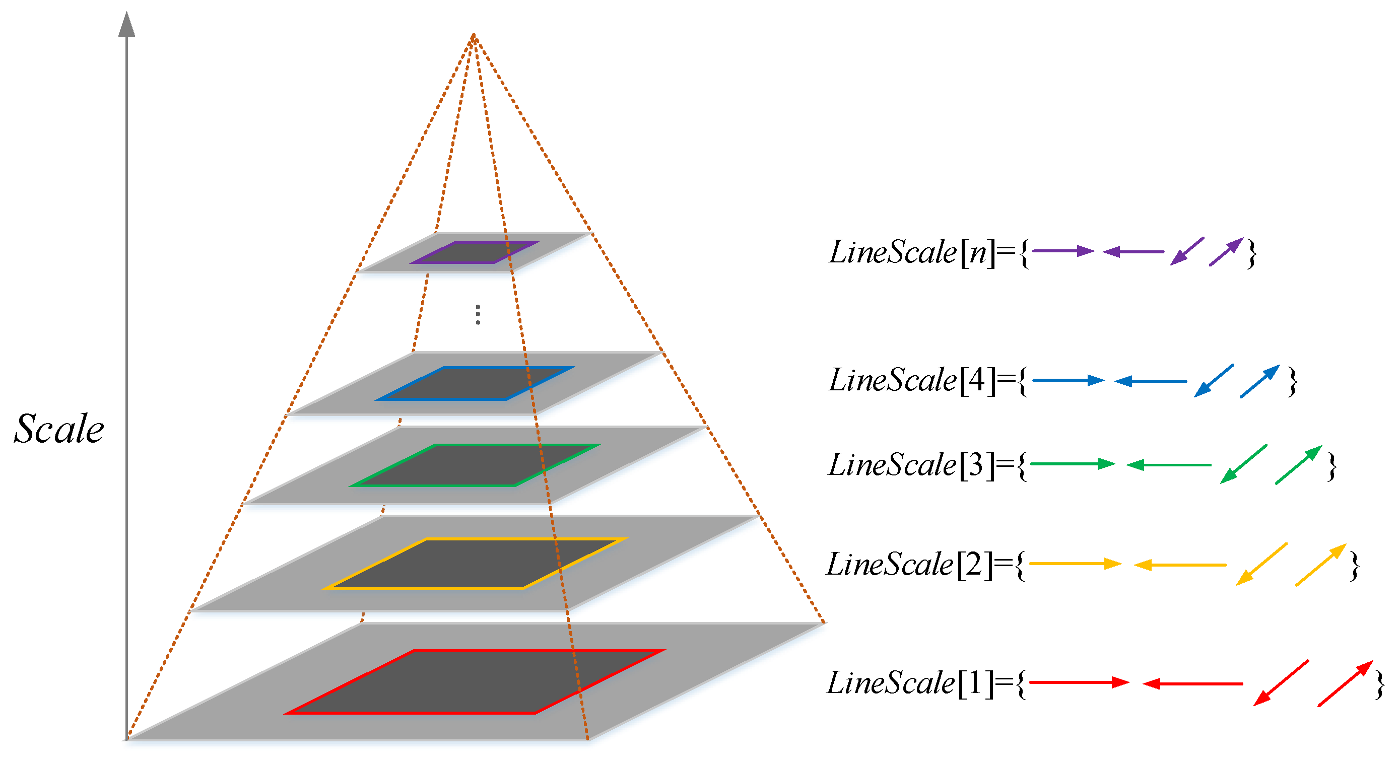
Figure 3.
Illustration of the banded sub-regions of line segment L. The small arrows represent the gradients of the pixels. The direction is defined as the average gradient orientation of all the pixels on segment L, and the direction is defined as the counterclockwise orthogonal direction of . The entire support region is divided into m banded sub-regions with gradually changing widths.
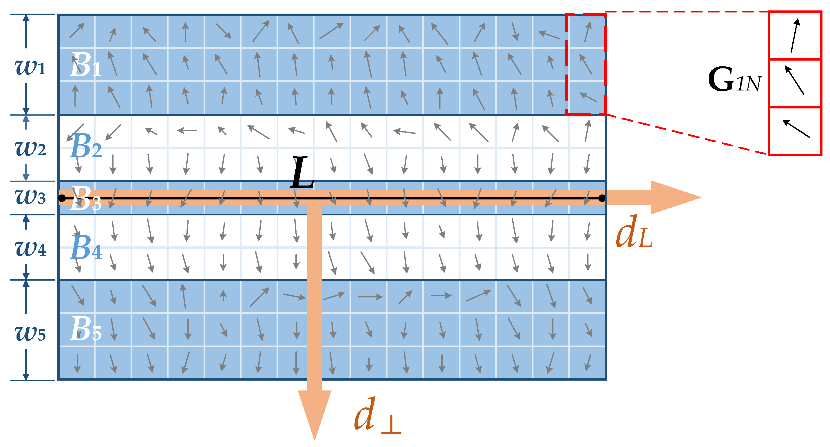
Figure 4.
Illustration of scale estimation in image pyramids. (a) Test image (left) and reference image (right); (b) Sum of the top 100 least Euclidean distances in nine scales.
Figure 4.
Illustration of scale estimation in image pyramids. (a) Test image (left) and reference image (right); (b) Sum of the top 100 least Euclidean distances in nine scales.

Figure 5.
Illustration of the proposed similarity metric (i.e., score of nearest pixels (SNP)). (a) 2D Gaussian distribution model; (b) The scoring model for SNP metric.
Figure 5.
Illustration of the proposed similarity metric (i.e., score of nearest pixels (SNP)). (a) 2D Gaussian distribution model; (b) The scoring model for SNP metric.

Figure 6.
Illustration of generating intersections using matching lines. (a) Test image with several line segments; (b) Reference image with corresponding line segments. The location constraint of intersections is marked as a red rectangular area (only shown in reference image in this example). Intersections satisfying the constraint are in green, otherwise in red.
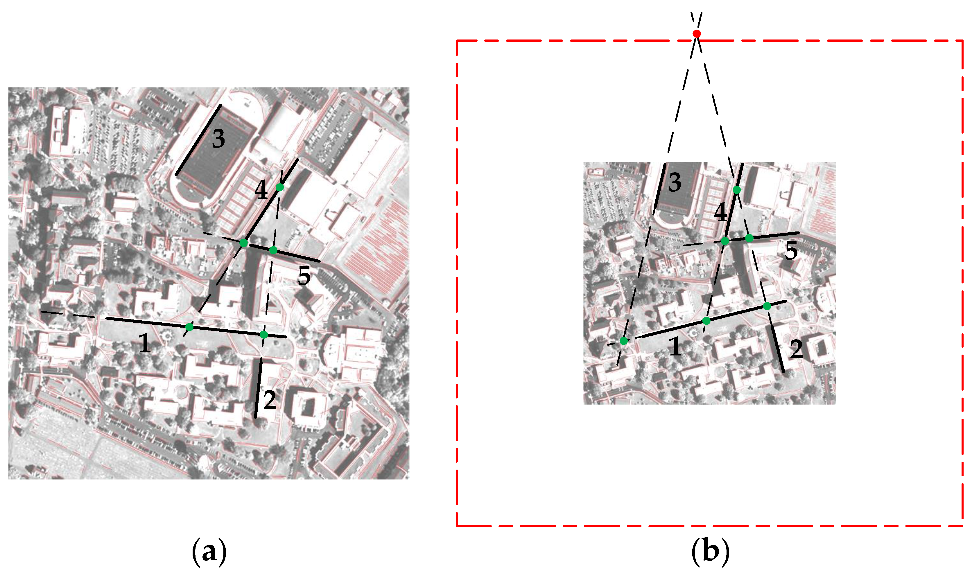
Figure 7.
Examples of synthetic images. (a) Panchromatic satellite image from WorldView-1; (b) the corresponding RGB image of (a) from QuickBird; (c) synthetic image with a scale ratio of 0.4; (d) synthetic image with a rotation angle of ; (e) synthetic image with considerably higher brightness than the original image; (f) synthetic image with mass cloud patches.
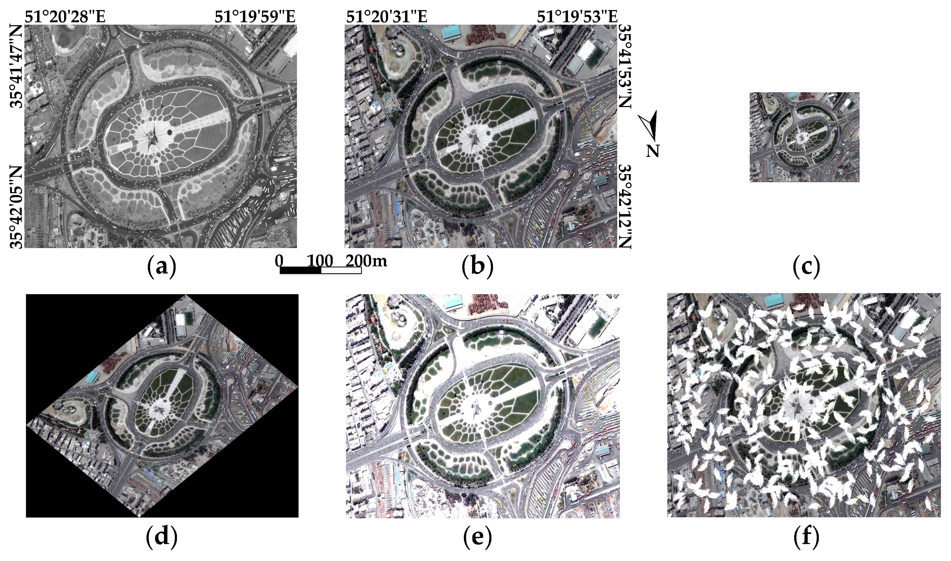
Figure 8.
Illustration of real image pairs. (a–d) show the image pairs from Data set 2-1 to Data set 2-4.
Figure 8.
Illustration of real image pairs. (a–d) show the image pairs from Data set 2-1 to Data set 2-4.

Figure 9.
Performances of the proposed RLI method in terms of root-mean-square error (RMSE) and number of correct matches over synthetic images under conditions of (a) scale, (b) rotation, (c) illumination, and (d) cloud cover.
Figure 9.
Performances of the proposed RLI method in terms of root-mean-square error (RMSE) and number of correct matches over synthetic images under conditions of (a) scale, (b) rotation, (c) illumination, and (d) cloud cover.

Figure 10.
Matching results of the proposed method on real image pairs. The lines connect matching intersection points on (a) Data set 2-1; (b) Data set 2-2; (c) Data set 2-3; (d) Data set 2-4.
Figure 10.
Matching results of the proposed method on real image pairs. The lines connect matching intersection points on (a) Data set 2-1; (b) Data set 2-2; (c) Data set 2-3; (d) Data set 2-4.

Figure 11.
Illustration of the registration results. (a) Results of mean-standard deviation line descriptor (MSLD) on Data set 2-1; (b) results of scale-invariant feature transform (SIFT) on Data set 2-2; (c) results of line matching leveraged by point correspondences (LP) on Data set 2-3; (d) results of RLI on Data set 2-1; (e) results of RLI on Data set 2-2; and (f) results of RLI on Data set 2-3.

Table 1.
Total number of correct matches with different parameters.
| Parameter Setting | Total Correct Matches | Descriptor Dimension | |
|---|---|---|---|
| m = 3 | 407 | 24 | |
| 502 | 24 | ||
| 541 | 24 | ||
| m = 5 | 898 | 40 | |
| 965 | 40 | ||
| 997 | 40 | ||
| m = 7 | 1212 | 56 | |
| 1325 | 56 | ||
| 1328 | 56 | ||
| m = 9 | 1350 | 72 | |
| 1524 | 72 | ||
| 1496 | 72 | ||
| m = 11 | 1433 | 88 | |
| 1613 | 88 | ||
| 1579 | 88 | ||
Table 2.
Characteristics of data sets.
| Types | No. | Location | Image Size | Bits | GSD(m) | Date | Sensor | Notes |
|---|---|---|---|---|---|---|---|---|
| Synthetic images | 1-1 | Iran | 11 | 0.5 | 2009 | WorldView-1 | Panchromatic | |
| 11 | 0.61 | 2009 | QuickBird | RGB | ||||
| Real images | 2-1 | Pakistan | 11 | 2 | 2010 | QuickBird | Post-flood | |
| 11 | 2 | 2007 | QuickBird | Pre-flood | ||||
| 2-2 | Fukushima | 8 | 10 | 2011 | SPOT4 | Post-tsunami | ||
| 8 | 10 | 2009 | SPOT4 | Pre-tsunami | ||||
| 2-3 | Myanmar | 8 | 231.65 | 2008 | Aqua | Pre-flood | ||
| 8 | 231.65 | 2008 | Aqua | Post-flood | ||||
| 2-4 | Chile | 11 | 0.61 | 2010 | QuickBird | Post-tsunami | ||
| 11 | 0.61 | 2010 | QuickBird | Pre-tsunami |
Table 3.
Experimental results of real remote sensing images.
| Method | Criteria | Data Set 2-1 | Data Set 2-2 | Data Set 2-3 | Data Set 2-4 |
|---|---|---|---|---|---|
| RLI | Correct matches | 88 | 9 | 11 | 8 |
| Precision (%) | 100 | 100 | 100 | 100 | |
| RMSE | 1.14 | 0.97 | 0.44 | 1.06 | |
| RMLSM | Correct matches | 20 | 31 | 65 | 21 |
| Precision (%) | 87.0 | 88.6 | 95.6 | 63.6 | |
| RMSE | 1.19 | 1.08 | 0.80 | 1.24 | |
| MSLD | Correct matches | 39 | 13 | 33 | 16 |
| Precision (%) | 60 | 37.1 | 61.1 | 45.7 | |
| RMSE | 1.41 | 1.55 | 0.86 | 1.38 | |
| SIFT | Correct matches | 163 | 44 | 151 | 12 |
| Precision (%) | 71.5 | 59.5 | 64.8 | 18.5 | |
| RMSE | 1.33 | 1.60 | 0.82 | 1.30 | |
| LP | Correct matches | 21 | 9 | 29 | 6 |
| Precision (%) | 34.4 | 31.0 | 87.9 | 24.0 | |
| RMSE | 1.21 | 1.28 | 1.18 | 1.20 |
Table 4.
Projected distance distribution of corresponding intersections of RLI.
| Projected Distance | Data Set 2-1 | Data Set 2-2 | Data Set 2-3 | Data Set 2-4 |
|---|---|---|---|---|
| 72 | 4 | 10 | 3 | |
| 16 | 2 | 1 | 5 | |
| 0 | 3 | 0 | 0 | |
| 0 | 0 | 0 | 0 |
© 2017 by the authors. Licensee MDPI, Basel, Switzerland. This article is an open access article distributed under the terms and conditions of the Creative Commons Attribution (CC BY) license (http://creativecommons.org/licenses/by/4.0/).
Share and Cite
MDPI and ACS Style
Lyu, C.; Jiang, J. Remote Sensing Image Registration with Line Segments and Their Intersections. Remote Sens. 2017, 9, 439. https://doi.org/10.3390/rs9050439
AMA Style
Lyu C, Jiang J. Remote Sensing Image Registration with Line Segments and Their Intersections. Remote Sensing. 2017; 9(5):439. https://doi.org/10.3390/rs9050439
Chicago/Turabian StyleLyu, Chengjin, and Jie Jiang. 2017. "Remote Sensing Image Registration with Line Segments and Their Intersections" Remote Sensing 9, no. 5: 439. https://doi.org/10.3390/rs9050439
Note that from the first issue of 2016, this journal uses article numbers instead of page numbers. See further details here.