Abstract
Recently, several methods have been introduced and applied to estimate daily air surface temperature (Ta) using MODIS land surface temperature data (MODIS LST). Among these methods, the most common used method is statistical modeling, and the most applied algorithms are linear/multiple linear regression models (LM). There are only a handful of studies using machine learning algorithm models such as random forest (RF) or cubist regression (CB). In particular, there is no study comparing different combinations of four MODIS LST datasets with or without auxiliary data using different algorithms such as multiple linear regression, random forest, and cubist regression for daily Ta-max, Ta-min, and Ta-mean estimation. Our study examines the mentioned combinations of four MODIS-LST datasets and shows that different combinations and differently applied algorithms produce various Ta estimation accuracies. Additional analysis of daily data from three climate stations in the mountain area of North West of Vietnam for the period of five years (2009 to 2013) with four MODIS LST datasets (AQUA daytime, AQUA nighttime, TERRA daytime, and TERRA nighttime) and two additional auxiliary datasets (elevation and Julian day) shows that CB and LM should be applied if MODIS LST data is used solely. If MODIS LST is used together with auxiliary data, especially in mountainous areas, CB or RF is highly recommended. This study proved that the very high accuracy of Ta estimation (R2 > 0.93/0.80/0.89 and RMSE ~1.5/2.0/1.6 °C of Ta-max, Ta-min, and Ta-mean, respectively) could be achieved with a simple combination of four LST data, elevation, and Julian day data using a suitable algorithm.
1. Introduction
Air surface temperature (Ta) with high spatial and temporal resolution plays an important role in various applications, such as crop growth monitoring and simulations [1], hydrological, ecological, and environmental studies [2,3,4], weather forecasting [5,6], and climate change [7,8]. It is used as a key input variable and directly affects the accuracy of these applications. Traditionally, Ta is usually measured by weather stations (often at 2 m above the ground) and usually limited in spatial coverage. Especially in mountainous areas of Vietnam, weather station coverage is extremely sparse.
Meanwhile, satellite data available at various spatial and temporal resolutions, such as Landsat, the Advanced Very High Resolution Radiometer (AVHRR), Advanced Spaceborne Thermal Emission and Reflection Radiometer (ASTER), and especially Moderate-resolution Imaging Spectroradiometer (MODIS), which was launched in the early 2000s, have marked a significant increase in the quality and quantity of thermal data. The advantage of MODIS is that it can provide Land Surface Temperature (LST) data directly. However, there is a difference between Ta and LST because of the complex surface energy budget and multiple related variables between them.
Recently, several methods have been introduced and applied to estimate Ta using satellite data such as the temperature–vegetation index method—TVX [9,10,11], surface energy-balance-based methods [12], and statistical methods [13,14,15,16,17,18] using different satellite datasets such as Landsat—ETM+ [19,20], AVHRR [21], or MODIS LST [11,14,22,23]. Among these satellite data, the most used is MODIS LST because it is freely available and can be obtained easily [18]. In addition, MODIS satellite provides four LST datasets daily, including: TERRA daytime (LSTtd), TERRA nighttime (LSTtn), AQUA daytime (LSTad), and AQUA nighttime (LSTan), which overpass local time at around 10 a.m., 10 p.m., 1 p.m., and 1 a.m. (our study area), respectively.
Looking at the current literature, there are plentiful Ta estimation studies; however, studies using machine learning techniques such as cubist regression (CB) or random forests (RF) are very rare (as far as we know, only [18,24,25,26]. However, all of these studies used MODIS LST integrating auxiliary data and estimated only Ta-max or Ta-mean. Furthermore, their conclusions are also different. Meyer et al. [26] stated that RF algorithms show the weakest results among linear regression, generalized boosted regression models (GBM), and Cubist regression. In contrast, Xu et al. [25] concluded that RF outperforms the linear regression. Zhang et al. [18] divided their data record into two groups (group S1 contains all four MODIS LST under good quality and group S2 had at least one LST with poor quality). The results based on the two datasets are different: in group S1, RF shows the best results in almost all combinations, but in group S2 the best algorithm is the Cubist regression. As a final result, the best algorithm for daily Ta-max, Ta-min, and Ta-mean estimation remains unknown.
Regarding MODIS LST data (v005), LST data are not available for a location (pixel) if cloudiness is present inside the pixel [27]. Due to the differences in satellite overpass times, the valid observation data at a specific location (pixel) varies between LSTad, LSTan, LSTtd, and LSTtn. Therefore, it is important to compare the dynamic combination of one to four LST data that are available at different times and locations as well as the most suitable algorithm to apply for Ta estimation. Furthermore, a rising question using LST MODIS solely is the kind of relationship (linear or nonlinear) between LST and Ta, especially in mountainous areas.
Therefore, in this research, we investigate all 15 (i.e., 24 − 1) possible dynamic combinations of four LST with or without auxiliary data for daily Ta estimation using three different algorithms: multiple linear regression (LM), cubist regression (CB), and random forests models (RF). Finally, the accuracies of these Ta-estimated are evaluated by comparison with Ta-measured data, which are collected from weather stations. Root mean square error (RMSE) and coefficient of determination (R2) were used as the model evaluation scores.
2. Materials and Methods
2.1. Study Area and Weather Station Data
The study area is located in northwest Vietnam inside two large provinces: Lai Chau and Dien Bien. It covers an area of 18,600 km2 (Figure 1). The study area presents a rural and mountainous region in northwest Vietnam with a sparse distribution of weather stations. There are only four weather stations (Figure 1) within these two provinces. However, due to the lack of data measurement, we chose only three stations, Sin Ho, Dien Bien, and Lai Chau, for this study (Table 1). In each station, the Ta data were recorded hourly. Ta-max and Ta-min are the highest (maximum) and lowest (minimum) air surface temperatures that occur on a diurnal cycle (24 h cycle), respectively; Ta-mean was calculated by averaging all 24 hourly measurements in a day. Generally, Ta-max occurs after solar noon from one to two hours, and Ta-min usually occurs shortly before dawn. In this study, we collected daily Ta-max, Ta-min, and Ta-mean from 2009 to 2013 from the Vietnam Institute of Meteorology, Hydrology, and the Environment (IMHEN).
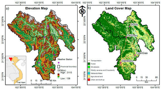
Figure 1.
Location of the weather stations and range of elevation (a) and land cover (b) from MODIS MCD12Q1 data in 2010 of the study area.

Table 1.
Geographical description and land cover type of weather stations used in this study.
Based on the MODIS land cover type product (MCD12Q1 data of 2010), the major land cover type in this area is forest, covering approximately 64% (Figure 1).
2.2. Data
2.2.1. MODIS LST
All MODIS LST data used in this study were acquired from the U.S. Geological Survey (USGS) website [28].
We used two MODIS LST products (v005, h27v06), MOD11A1 and MYD11A1 from TERRA and AQUA satellites, respectively. The MODIS LST consists of daytime and nighttime data at a spatial resolution of 1 km. Thus, in total there are four LST datasets: AQUA daytime (LSTad), AQUA nighttime (LSTan), TERRA daytime (LSTtd), and TERRA nighttime (LSTtn).
In the literature, there are some studies that use eight-day LST averages to estimate Ta [13,14,29]. It should be considered that eight-day-average LST is calculated by averaging all valid data under clear sky conditions, the number of participant data points varying from one to eight days depending on availability. Meanwhile, eight-day-average Ta is calculated by averaging the data under changing sky conditions. Therefore, if we compare eight-day-average LST and eight-day-average Ta, the sampling may introduce uncertainty [22]. Taking this difference into consideration, in this study we decided to use daily LST under clear sky conditions instead of eight-day-average LST data.
2.2.2. MODIS Land Cover
The MODIS Land Cover Type Product (MCD12Q1) is downloaded from the Land Processes Distributed Active Archive Center [30]. In order to use this product easily in the community, four main classification schemes were provided, including IGBP (International Geosphere–Biosphere Programme), UMD (University of Maryland), LAI/fPAR (Leaf Area Index/fraction of Photosynthetically Active Radiation), and NPP (Net Primary Productivity) [30,31]. For our study, we use the primary land cover scheme, which is provided by the IGPB land cover classification. Based on this scheme, our study has 13 types of land cover classes. However, in order to make it easy to use and distinguish between each class, consistent with the land cover of the study area we combined and reduced the classes to six types (Figure 1). As is shown in Figure 1, the majority of land cover in the study area is forest and crop land.
In addition, based on the results of our previous study [17], we take two more variables into account for Ta estimation in northern Vietnam: station elevation (el) and Julian day data. Elevations of stations were obtained from the Vietnam Institute of Meteorology, Hydrology and Environment (IMHEN). The Julian day (jd) was extracted from the NASA server [32].
2.3. Methods
2.3.1. Calculating LST of Weather–Station–Location
LST data under clear sky conditions at weather stations are retrieved by the following steps:
- A total of 3652 MODIS images (MOD11A1 and MYD11A1, h27v06, Collection 5, from 1 January 2009 to 31 December 2013, over northern Vietnam) in HDF (Hierarchical Data Format) format were reprojected to WGS_1984_UTM_zone_48N using the nearest neighbor resampling method with the MODIS Re-Projection Tool. The corresponding layers (LST_Day_1km, LST_Night_1km, Daytime LST observation time, and Nighttime LST observation time) were extracted in TIF format. However, Daytime and Nighttime LST observation time were used in order to identify the approximate overpass time of MODIS at local time.
- MODIS LST data for the pixels in which the weather stations are located are extracted from 7304 TIF format MODIS images (3652 daytime and 3652 nighttime images) using batch processing of extract multi value to points in ArcGIS 10.3.
- All these LST data (DN value) were converted to Celsius temperature using the following equation:where °C is the Celsius temperature and 0.02 is the scale factor of the MODIS LST product.°C = 0.02 * DN − 273.15,
- Removing outlier data: MODIS LST products are not available for a location (pixel) if clouds are present [27]. However, there are some pixels that are lightly covered or contaminated by clouds. These pixels are not removed because the contamination is very small and cannot be detected by the cloud-removing mask algorithm [33,34]. To avoid this kind of data, we studied and developed a similar method that was used in [35]. This approach includes two steps: First, we simply filter and remove all unrealistic LST data that had values greater than 100 °C and/or below −50 °C. Second, we calculated the difference between Ta-max versus LST daytime and Ta-min versus LST nighttime. Then, we applied statistical outlier removal based on these differences’ histograms to detect and remove data with unusually large differences (the histogram does not follow a normal distribution).
2.3.2. Estimation Air Temperature Using MODIS LST Data
- Dynamic Combination of MODIS LST data
To estimate daily Ta, we used all possible combinations of four LST data (LSTad, LSTan, LSTtd, and LSTtn). These 15-combinations are shown in Table 2.
Table 2.
All possible combinations of four LST data and the valid number of observations.
Due to the cloud cover effect, the number of valid observations from each station and each combination (C01–C15) are various (Table 2).
In order to investigate the difference between dynamic combinations, as well as the performance of different algorithms, we used two datasets: Dataset A, MODIS LST data only; and Dataset B, MODIS LST together with elevation (ele) and Julian day (jd) data.
- Algorithms used
Linear/Multiple Linear Regression Model (LM) is a model that represents the relationship between one response variable and one predictor variable (Simple Linear Regression) or more than one predictor variable (Multiple Linear Regression) by using parameters entered linearly and estimated by the least squares method. So far, LM is one of the most popular statistical models for Ta estimation using MODIS LST [14,17,22,25,36,37]. Although it was found that the correlation between LST and Ta is high, this relationship may not actually be linear [18]. Therefore, our current knowledge might be incomplete if we do not try machine learning algorithms. Machine learning algorithms promise a better estimation of Ta using MODIS LST because they can handle non-linearity and highly correlated predictor variables [26,38,39]. Furthermore, based on the conceptual designs of machine learning algorithms, they are able to deal with data that have a different relationship between predictor and response variables under different conditions such as season, elevation, and land cover characteristic [26].
Random Forests (RF), which was proposed by Breiman in 2001 [40], is a nonparametric and ensemble technique. Random forests are a combination of tree predictors such that each tree depends on the values of a random vector sampled independently and with the same distribution for all trees in the forest. It is different from traditional statistical methods that contain a parametric model for prediction. In RF, it contains many decision trees, where each tree is built from a random subset of training data with a random subset of predictor variables. The final predicted values are produced by the aggregation of the results of all the individual trees that make up the forest [25].
Cubist regression (CB) is a rule-based regression technique that was developed based on a combination of the ideas of Quinlan [41,42,43]. CB does not retrieve one final model like RF, but a set of rules associated with sets of multi-variate models. Then, a specific set of predictor variables will choose an actual prediction model based on the rule that best fits the predictors [44]. Cubist is a commercial, proprietary product and has the least algorithmic documentation in comparison to linear regression and random forest [45]. However, it is currently a popular and widely used regression and classification method because it was ported into R by Kuhn et al. [46] in 2013. Most recently, it was used in Ta estimation research and showed very good results in the research of Meyer et al. [26] and Zhang et al. [18].
Therefore, in this study, to estimate Ta and assess the accuracy of estimation, three different methods were employed: linear regression (LM), cubist regression (CB) and random forests (RF). All methods are performed in the R statistical software.
2.3.3. Comparison of Different Combination and Algorithms
- Assessment Criteria
To assess the performance of models, we used and compared the values of the two most popular criteria: the coefficient of determination (R2) and the root mean square error (RMSE) that were calculated from the measured and estimated Ta values from three algorithms: LM, CB, and RF.
- Comparison
Being one of the most popular validation methods, cross-validation was used in order to compare different combinations and different algorithms.
In order to implement the cross-validation, the dataset is divided into k groups (k-fold) of approximately the same size. Then, k − 1 groups of the dataset are used as the training set, and the left-out group is used for validation. When the number of groups (k) equals the number of observations (n), it is called “leave-one-out cross-validation”.
Due to the high number of observations, we used 10-fold cross-validation (k = 10) and repeated it twice for cross-validation.
3. Results
3.1. The Relationship between Ta and LST MODIS
In order to evaluate the MODIS LST data for Ta estimation, we first test the relationship between Ta and LST MODIS of all three weather stations.
Figure 2 shows the scatter plot of Ta and LST of daytime and nighttime. It was found that: The coefficients of determination were high, ranging from 0.43 to 0.72, and the correlation between LST nighttime and Ta-min were higher than LST daytime and Ta-max at Dien Bien and Sin Ho stations. However, at Lai Chau station, the correlation between LST daytime versus Ta-max was slightly higher than nighttime versus Ta-min. This indicates that the relationship between MODIS LST and Ta of this study area is complex.
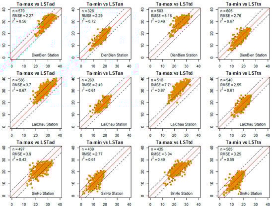
Figure 2.
The relationship between LST (x-axis) and Ta-max (first and third columns), Ta-min (second and last columns) of all meteorological stations from 2009 to 2013. The dashed line indicates that the difference between Ta and LST is over ±5 °C (±5 line). The red line indicates the 1:1 line.
The relationships between Ta-min versus LSTan and LSTtn were quite similar at all three stations. However, the relationships between Ta-max versus LST daytime were different; at Lai Chau station most Ta-max values are higher than the LSTad and LSTtd values (most of the points lie above the red line). Meanwhile, at Dien Bien station, Ta-max is quite similar to LSTad but Ta-max was higher than LSTtd. At Sin Ho station, there is not much difference between Ta versus LST but there are a lot of data points lying outside the “±5 lines”.
Due to the cloud effect, the number of valid observations changes from daytime to nighttime; during the daytime the AQUA sensor gives more observations than TERRA. However, at night, TERRA gives more observations than AQUA.
3.2. Different Combinations of MODIS LST for Ta Estimation
As shown in Figure 2, the linear correlation between Ta and LST are strong for both Terra LST and Aqua LST of daytime and nighttime. Furthermore, in Section 1 we also showed that there are plenty of studies using MODIS LST data for Ta estimation using the LM method.
Therefore, in order to estimate the effect of different MODIS LST data combinations, we applied all three methods (linear regression, cubist regression, and random forest models) to the 15 combinations as shown in Table 2.
In the LM method, the equations of 15 combinations (C01–C15) are shown in Appendixe A and Appendixe B. However, regarding CB and RF, which are nonparametric methods, equations cannot be provided as for the LM method.
3.2.1. Combinations Using One LST Variable
Figure 3a,b show the coefficient of determination (R2) and root mean square error (RMSE) of combinations C01–C04 using three algorithms (LM, CB, and RF) with Dataset A and Dataset B, respectively. It can be clearly seen that there is a large difference between Figure 3a (using LST solely) and Figure 3b (using LST with elevation and Julian day data). At Figure 3a, LM and CB show similar results and higher accuracy than the RF algorithm in all four combinations (C01–C04). In contrast, Figure 3b shows similar results for CB and RF in all four combinations and slightly higher values than with the LM algorithm. It is suggested that when one LST is used with an auxiliary data for Ta estimation, RF and CB performance are better than LM.
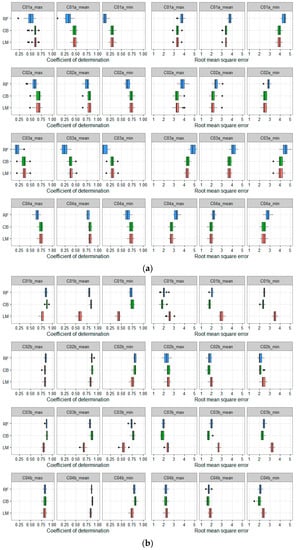
Figure 3.
(a) Cross-validation results for one-LST-combination (C01–C04) using Dataset A, and multiple comparisons of the three algorithms. The x-axis shows the value of R2 and RMSE (°C), the y-axis shows the model types. The box and whiskers plots show the distributions of R2 and RMSE; (b) Cross-validation results for one-LST-combination (C01–C04) using Dataset B, and multiple comparisons of the three algorithms. The x-axis shows the values of R2 and RMSE (°C); the y-axis shows the model types. The box and whiskers plots show the distributions of R2 and RMSE.
Both Figure 3a,b show that the accuracy of C02 and C04 is much higher than for C01 and C03 (higher value of R2 and lower value of RMSE). It can be stated that nighttime LST was better than daytime for deriving daily Ta. This result is consistent with [17,47]. Regarding the two datasets used, in all combinations (C01–C04) the accuracies of Ta estimation using Dataset B are much higher than when using Dataset A.
For Ta-min and Ta-mean estimation, Figure 3a shows that the combinations using LST nighttime (C02 and C04) have significantly higher accuracy than the combinations using LST daytime (C01 and C03). However, these differences are not clearly shown in Figure 3b (except for in the LM results).
Regarding Dataset A, AQUA daytime (C01) shows better results for Ta-max estimation than TERRA daytime (C03). However, at night AQUA and TERRA show similar results for Ta estimation. The results of both daytime and nighttime of TERRA and AQUA are consistent and similar in Ta estimation (Figure 3b).
3.2.2. Combinations Using Two-LST Variables
In this case, we used all possible combinations with LST to estimate Ta. As shown in Table 2, we applied six possible combinations of LST for Ta estimation.
In general, Figure 4a,b show that both results of Ta estimation using Dataset A and B are higher than the one-LST-combination (Figure 3a,b). Figure 4a shows that the difference between the three algorithms is not as large as in the results shown in Figure 3a (except for C07).
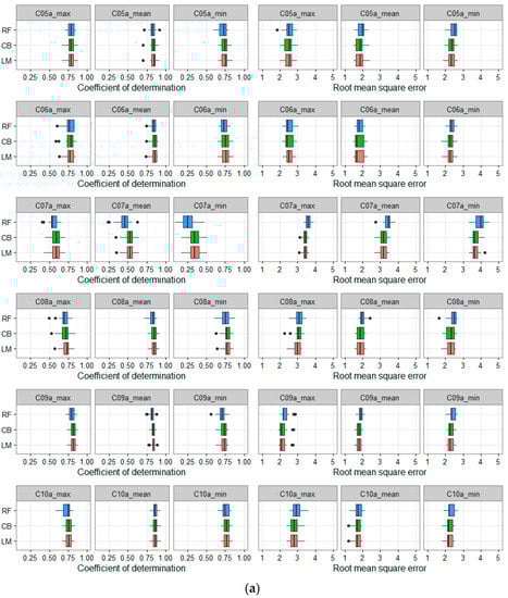
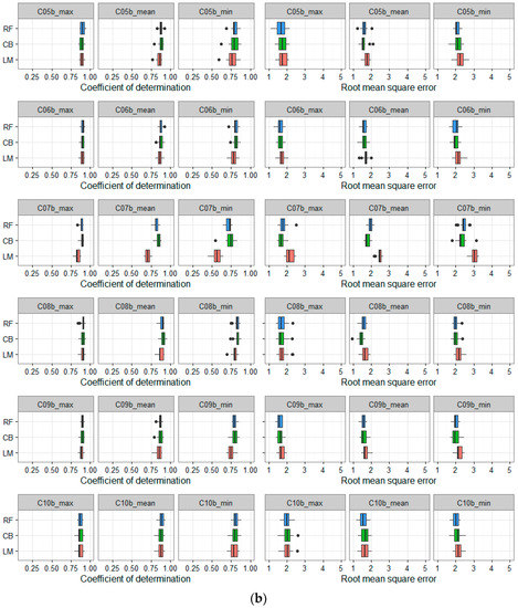
Figure 4.
(a) Cross-validation results for two-LST-combinations (C05–C10) using Dataset A and multiple comparisons of the three algorithms. The x-axis shows the value of R2 and RMSE (°C); the y-axis shows the model types. The box and whiskers plots show the distributions of R2 and RMSE; (b) Cross-validation results for two-LST-combinations (C05–C10) using Dataset B and multiple comparisons of the three algorithms. The x-axis shows the values of R2 and RMSE (°C); the y-axis shows the model types. The box and whiskers plots show the distributions of R2 and RMSE.
In these combinations (C05–C10), CB and LM show similar and slightly higher accuracies than RF for Dataset A. The contrast is also evident in Dataset B: the CB and RF results are similar and slightly higher than LM. Especially in C07, the results of LM are much lower than those of CB and RF (Figure 4b). The results of all Ta estimations using Dataset B are still higher than using Dataset A.
Looking at the first two rows of Figure 4a,b (C05, combined LSTad + LSTan; and C06, combined LSTtd + LSTtn), there are similar results for Ta estimations between them. It is indicated that the overpass times of AQUA and TERRA do not significantly affect the result of Ta estimation when we combine daytime and nighttime LST. This is true for all three methods (LM, CB, and RF). These results are also consistent with previous studies [15,17,47], which used LM as the statistical model for Ta estimation.
The most interesting finding of two-LST-combined is the combination of C07. The results of Dataset A (panel row 3, Figure 4a) show the lowest accuracy in comparison to five other two-LST-combined (R2 approximately 0.6, 0.5 and 0.35; RMSE approximately 3.5, 3.2, and 3.7 °C for Ta-max, Ta-mean, and Ta-min, respectively). In addition, among the three algorithms, RF shows the lowest results with lower R2 and higher RMSE. In contrast, the results of Dataset B are absolutely different (Figure 4b, panel row 3). The results of C07 (using Dataset B) are similar to the five other two-LST-combined (R2 approximately 0.88, 0.80, and 0.73; RMSE approximately 1.8, 1.9, and 2.5 °C for Ta-max, Ta-mean, and Ta-min, respectively, except for the results of LM) and much higher than using Dataset A. Among the three algorithms, the lowest result for Ta estimation is LM (Figure 4b). Meanwhile, CB and RF show higher results, especially for Ta-min and Ta-mean estimation. It should be noted that C07 is the combination of TERRA and AQUA daytime LST, which is the most complicated in the relationship between Ta and LST in comparison to the rest of the combinations. The difference between the results of Datasets A and B indicates that elevation and Julian day (i.e., season) also affect the relationship between LST and Ta. This is consistent with the results from [15,23,48,49]. The high accuracy of Ta estimation using the RF and CB algorithms in Figure 4b also indicates that RF and CB can account for the complicated relationship between predictor and response variables under different conditions, especially in mountainous area. This finding is consistent with the studies by Zhang et al. [18] and Xu et al. [25].
3.2.3. Combinations Using Three-LST Variables
In general, Figure 5a,b show that all three-combined LST result in a very high accuracy of Ta estimation and the differences in accuracy between the three different algorithms are not significant (p-value > 0.05). However, the results of Ta estimation using Dataset B are much higher than using Dataset A. In both datasets, the results of Ta-max and Ta-mean are always better than Ta-min (except C12 and C14 of Dataset A). This can be explained by the fact that, because of two LST nighttime variables (LSTtn and LSTan) in C12 and C14, the accuracy of Ta-min estimation could be increased. However, in Dataset B, by introducing the two variables elevation and Julian day, the accuracy of all Ta-max, Ta-min, and Ta-mean estimations has increased (Ta-max and Ta-mean is increased more significantly than Ta-min when elevation and Julian day data were introduced).
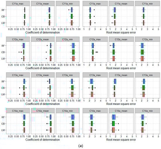

Figure 5.
(a) Cross-validation results for three-LST-combinations (C11–C14) using Dataset A and multiple comparisons of the three algorithms. The x-axis shows the values of R2 and RMSE (°C); the y-axis shows the model types. The box and whiskers plots show the distributions of R2 and RMSE; (b) Cross-validation results for three-LST-combinations (C11–C14) using Dataset B and multiple comparisons of the three algorithms. The x-axis shows the value of R2 and RMSE (°C); the y-axis shows the model types. The box and whiskers plots show the distributions of R2 and RMSE.
3.2.4. Combinations Using Four-LST Variables
The first result clearly seen from Figure 6 is that all three algorithms show a similar accuracy of Ta estimation in both Dataset A and B. However, the results of Dataset B (R2 approximately 0.93, 0.89 and 0.8, RMSE approximately 1.5, 1.6, and around 2.0 °C for Ta-max, Ta-mean, and Ta-min, respectively) are much higher than the results of Dataset A (R2 approximately 0.84, 0.88, and 0.75; RMSE roughly 2.2, 1.7, and 2.2 °C for Ta-max, Ta-mean, and Ta-min, respectively).
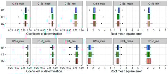
Figure 6.
Cross-validation results for four-LST-combinations (C15) using Dataset A (upper rows) and B (lower rows) and multiple comparisons of the three algorithms. The x-axis shows the values of R2 and RMSE (°C); the y-axis shows the model types. The box and whiskers plots show the distributions of R2 and RMSE.
In addition, the statistical results also indicate that the difference between the three algorithms is not significant (p-value > 0.05) in either Dataset A or B.
4. Discussion
4.1. Model Calibration and Validation
In several previous studies [23,36], one of the most common validation methods is that the sample data is randomly divided into a calibration and a validation dataset (e.g., 70% and 30% respectively). Calibration data were used for training data and validation data were used to assess the model performance. However, there is a drawback with this random choice: If we use a local dataset to train the model (i.e., a dataset that does not represent all dataset characteristics), then we apply a fitted model to the validation data. This could be misleading in the accuracy assessment. Especially in machine learning algorithms like CB or RF, this could lead to overfitting problems (e.g., the accuracy of the training part is very high; however, the model cannot be applied successfully to the validation dataset).
In this paper, we studied this problem in Ta estimation using MODIS LST. First, we randomly divide the data of all 15 combinations into two datasets: calibration and validation (70% and 30%, respectively). Next, we fitted the model using a calibration dataset, and then we applied the fitted model to the validation dataset and the entire dataset. Finally, we assessed the accuracies of validation data, full data, and cross-validation.
These processes are applied to both Dataset A and Dataset B.
In Figure 7, the LM algorithm shows consistent results between the validation data, the total data, and the cross-validations of both Dataset A and B. The results of Ta estimation using Dataset B (right-hand panel) are slightly higher than with Dataset A (left-hand panel). It could be suggested that when LST data alone were used (without auxiliary data), the accuracy of Ta estimation could be affected by a change in season or the elevation of the weather station. This is consistent with previous studies [17,36]. In the CB method (Figure 8), the results of validation, full data, and cross-validation are also consistent with each other. However, in both algorithms LM and CB, the results of Dataset A and Dataset B showed a significant difference, especially the combinations 1, 3, and 7 (C01, C03, and C07), where there is only LST daytime data. It is suggested that if LST nighttime is not available then the accuracy of Ta estimation could be improved by adding auxiliary data. Comparing Figure 7 and Figure 8, it can be clearly seen that CB produces better results for Ta estimation than LM.
Figure 7.
Comparison of accuracy (R2 and RMSE) when applying the LM algorithm to the validation dataset (_val), the full dataset (_all), and a cross-validation (_cv) of all combinations. The x-axis shows the combination number. The y-axis shows the values of RMSE (°C) and R2.
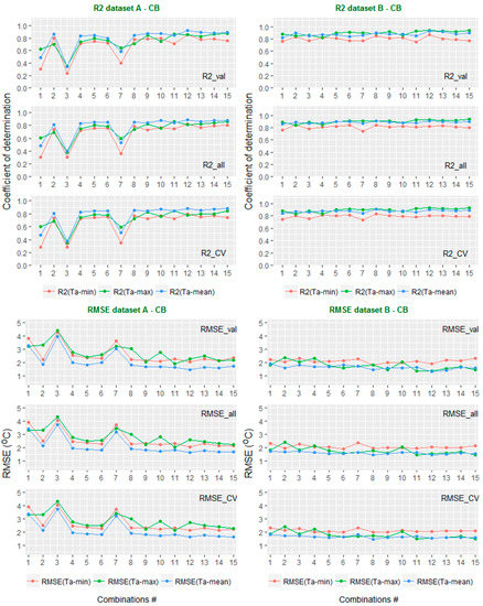
Figure 8.
Comparison of accuracy (R2 and RMSE) when applying the CB algorithm to the validation dataset (_val), the full dataset (_all), and a cross-validation (_cv) of all combinations. The x-axis shows the combination number. The y-axis shows the values of RMSE (°C) and R2.
Unlike LM and CB, the results of RF algorithm (Figure 9) are not consistent when applied to the validation data, full data, and cross-validation using Dataset A or Dataset B. As is shown in Figure 9, the results of cross-validation and the results using the validation data are similar and lower than when using the full data. It is suggested that the RF algorithm could be overfitting the Ta estimation using MODIS LST. It is also clearly seen that the results of Ta estimation using Dataset B are much higher than Dataset A, especially the combinations C01, C03, and C07. Again, the results of RF confirm that auxiliary data (i.e., elevation and Julian day) together with the RF algorithm can increase the accuracy of Ta estimation, especially in the case of missing LST nighttime data (i.e., combinations C01, C03, and C07).
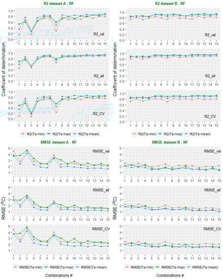
Figure 9.
Comparison of accuracy (R2 and RMSE) when applying the RF algorithm to the validation dataset (_val), the full dataset (_all), and a cross-validation (_cv) of all combinations. The x-axis shows the combination number. The y-axis shows the values of RMSE (°C) and R2.
4.2. Effects of Different Combinations and Statistical Model Applications
Figure 10 shows a comparison between the 15 combined LST datasets when applied to three different algorithms (LM, CB, and RF), based on the criteria of R2 and RMSE.
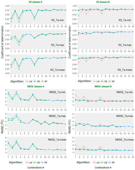
Figure 10.
Different performance of the algorithms LM (red), CB (green), and RF (blue) through 15 combinations of Dataset A and Dataset B. The x-axis shows the combination number. The y-axis shows the values of RMSE (°C) and R2.
Regarding Dataset A, in all combinations (C01–C15) for all Ta-max, Ta-min, and Ta-mean estimations, the results of the LM and CB algorithms are similar and higher than RF. However, from C10 to C15, the differences between the three algorithms are not clear. The results of combinations C01, C03, and C07 are much lower than the rest of the combinations in all three algorithms.
Considering Dataset B, the results are very different to those of Dataset A. Especially, in combinations C01, C03, and C07, the results of CB and RF are similar and much higher than LM. This can be explained by the fact that during the daytime, solar radiation affects the thermal infrared signal, and the relationship between Ta and LST becomes more complicated. That is why simple models like C01, C03, and C07 (of Dataset A) cannot handle this relationship well. The results of all combinations (C01 to C15) were quite similar when the CB and RF algorithms were applied.
It can be clearly seen that, in all combinations (C01–C15) of Dataset B, the cubist regression always shows the highest accuracy of Ta estimation (slightly higher than RF and much higher than LM). This is consistent with the studies of [18,25]. It should be remembered that Xu et al. [25] used MODIS LST and many other auxiliary variables like NDVI, longitude, latitude, etc. In this case, it could be explained by the complex terrain of the study area. It is suggested that the differences in topography, land surface properties, solar radiation, and many other factors could affect the relationships between Ta and LST [14,50,51,52]. Therefore, a linear regression model, considered as a single global model, could not handle the complicated relationship between Ta and the abovementioned variables under different conditions [25]. In contrast, CB and RF can account for the nonlinear and complicated relationship between the predictor and response variables under different conditions. That is why, in this mountainous study area, the cubist regression and random forest algorithms always show better results than LM in all 15 combinations (Figure 10, right panel).
However, from combination number C02 and C04 to 15 (except number 7—C07), which have at least one nighttime LST term in the combination, the performances of all three methods are good (high correlation and low errors).
Another point is that in Dataset A, the different combinations of LST had a similar effect on all three algorithms. However, in Dataset B, the different combinations of LST had a similar effect on RF and CB but a significantly different effect on the LM algorithm. The largest difference was found in Ta-min estimation, follow by Ta-mean and Ta-max estimation.
5. Conclusions
This study proved that the very high accuracy of Ta estimation (R2 > 0.93/0.80/0.89 and RMSE ~1.5/2.0/1.6 °C of Ta-max, Ta-min, and Ta-mean, respectively) could be achieved with a simple combination of four LST data, elevation, and Julian day data using a suitable algorithm.
Using Dataset B (MODIS LST, elevation, and Julian day) with RF or CB algorithms would give a stable and high accuracy in all combinations (C01–C15). With the LM algorithm, the more LST terms (especially LST nighttime) are presented the higher the accuracy that can be achieved.
The impact of the different combinations is larger in Dataset A than in Dataset B. However, in Dataset B, this impact was also large when using the LM algorithm.
LST nighttime data of both AQUA and TERRA play an important role in daily Ta estimation, guaranteeing higher accuracy. Depending on LST data availability, it could be used in any combination from C02, C04, and C05 to C15 (except C07 and C09) to achieve the highest results solely with MODIS LST using any of the three mentioned algorithms. However, when MODIS LST and auxiliary (elevation and Julian day) are available, any combination (C01–C15) can be applied with the CB or RF algorithm.
Among Ta-max, Ta-min, and Ta-mean, using Dataset A, Ta-mean was estimated with the highest accuracy, followed by Ta-min and Ta-max. However, the difference between Ta-max and Ta-min was not significant. Considering Dataset B, Ta-max was estimated with the highest accuracy, followed by Ta-mean and Ta-min. This means that the highest improvement for Ta-max is made by introducing elevation and Julian day data, followed by Ta-mean and Ta-min. However, the difference between Ta-max and Ta-mean was not significant.
Acknowledgments
We would like to acknowledge the Vietnamese government for its financial support and the Vietnam Institute of Meteorology, Hydrology, and the Environment (IMHEN) for supplying the meteorological data for this research. This publication was supported financially by the Open Access Grant Program of the German Research Foundation (DFG) and the Open Access Publication Fund of the University of Göttingen. We also thank the three anonymous reviewers for their valuable comments, which greatly improved our paper.
Author Contributions
The first author analyzed the data and performed the experiments; he also computed the statistical analysis in R-software. The second author helped to conceive and design the statistical analysis. The third author contributed analysis tools and corrected the final manuscript. All authors together developed and discussed the manuscript and finally wrote the paper.
Conflicts of Interest
The authors declare no conflict of interest.
Appendix A
Table A1.
Parameters of LM models for Ta estimation using Dataset A.
Table A1.
Parameters of LM models for Ta estimation using Dataset A.
| Combination | a0 | a1 | a2 | a3 | a4 | |
|---|---|---|---|---|---|---|
| Ta-min Estimation | C01 | −0.4567 | 0.6037 | |||
| C02 | −0.2678 | 1.0020 | ||||
| C03 | −1.1905 | 0.7170 | ||||
| C04 | −1.7601 | 1.0184 | ||||
| C05 | 0.1561 | −0.0656 | 1.0647 | |||
| C06 | −3.6700 | 0.0382 | 1.0329 | |||
| C07 | −4.1084 | 0.4906 | 0.2442 | |||
| C08 | −1.4168 | 1.0031 | 0.0277 | |||
| C09 | −2.1783 | −0.0425 | 1.0769 | |||
| C10 | −2.2857 | 0.4799 | 0.5784 | |||
| C11 | −2.8733 | −0.0336 | 0.0347 | 1.0349 | ||
| C12 | −2.4495 | 0.5464 | −0.0378 | 0.5552 | ||
| C13 | −1.0977 | −0.0344 | 0.9997 | 0.0496 | ||
| C14 | −0.5283 | −0.1538 | 0.6645 | 0.5408 | ||
| C15 | −1.6045 | −0.0714 | 0.6659 | −0.0020 | 0.4556 | |
| Ta-max Estimation | C01 | 0.7418 | 0.9849 | |||
| C02 | 8.4402 | 1.1748 | ||||
| C03 | 6.1865 | 0.9026 | ||||
| C04 | 5.8675 | 1.2125 | ||||
| C05 | −0.0367 | 0.5587 | 0.7505 | |||
| C06 | 4.3759 | 0.1263 | 1.1694 | |||
| C07 | −0.0708 | 1.0098 | −0.0068 | |||
| C08 | 8.5918 | 1.1432 | 0.0458 | |||
| C09 | −0.7751 | 0.4757 | 0.8778 | |||
| C10 | 5.5651 | 0.3821 | 0.9083 | |||
| C11 | 1.0850 | 0.5573 | −0.2434 | 0.9824 | ||
| C12 | 7.5080 | 0.4518 | −0.1274 | 0.9481 | ||
| C13 | 3.7089 | 0.6542 | 0.8513 | −0.3246 | ||
| C14 | −1.1526 | 0.4704 | 0.3212 | 0.6027 | ||
| C15 | 3.2723 | 0.5978 | 0.4074 | −0.4465 | 0.7015 | |
| Ta-mean Estimation | C01 | −0.3329 | 0.7579 | |||
| C02 | 3.0973 | 1.0630 | ||||
| C03 | 0.9103 | 0.8154 | ||||
| C04 | 1.1378 | 1.0888 | ||||
| C05 | −0.4702 | 0.2122 | 0.9074 | |||
| C06 | −1.6236 | 0.1523 | 1.0316 | |||
| C07 | −3.2005 | 0.6693 | 0.1964 | |||
| C08 | 1.3821 | 1.0028 | 0.1121 | |||
| C09 | −2.2374 | 0.1935 | 0.9691 | |||
| C10 | 0.7231 | 0.4639 | 0.6828 | |||
| C11 | −2.3500 | 0.2016 | 0.0036 | 0.9516 | ||
| C12 | −0.0214 | 0.5094 | 0.0377 | 0.6325 | ||
| C13 | −0.2995 | 0.2344 | 0.8818 | −0.0172 | ||
| C14 | −1.5659 | 0.1396 | 0.5060 | 0.5450 | ||
| C15 | −1.1587 | 0.1968 | 0.5392 | −0.0702 | 0.4952 |
a0 is the intercept of each model (combination), a1–a4 are parameters of LST variables with the same order as shown in Table 2.
Appendix B
Table A2.
Parameters of LM models for Ta estimation using Dataset B.
Table A2.
Parameters of LM models for Ta estimation using Dataset B.
| Combination | a0 | a1 | a2 | a3 | a4 | Elevation | Julian Day | |
|---|---|---|---|---|---|---|---|---|
| Ta-min Estimation | C01 | 4.1126 | 0.4728 | −0.0029 | 0.0066 | |||
| C02 | 0.3258 | 0.9505 | −0.0008 | 0.0057 | ||||
| C03 | 3.1331 | 0.6298 | −0.0042 | 0.0046 | ||||
| C04 | −1.6854 | 0.9873 | −0.0005 | 0.0050 | ||||
| C05 | 0.4293 | −0.0318 | 0.9822 | −0.0007 | 0.0050 | |||
| C06 | −4.5116 | 0.1075 | 0.9595 | −0.0006 | 0.0053 | |||
| C07 | 1.7992 | 0.0921 | 0.5553 | −0.0041 | 0.0042 | |||
| C08 | −1.4452 | 0.9067 | 0.0887 | −0.0009 | 0.0054 | |||
| C09 | −2.3238 | 0.0098 | 0.9868 | −0.0007 | 0.0049 | |||
| C10 | −2.7464 | 0.4843 | 0.5678 | −0.0003 | 0.0056 | |||
| C11 | −3.0229 | −0.0266 | 0.1405 | 0.8891 | −0.0011 | 0.0045 | ||
| C12 | −3.2945 | 0.5450 | −0.0031 | 0.5286 | −0.0003 | 0.0053 | ||
| C13 | −0.7924 | −0.0512 | 0.8894 | 0.1366 | −0.0010 | 0.0044 | ||
| C14 | −0.7538 | −0.1054 | 0.6304 | 0.4971 | −0.0005 | 0.0044 | ||
| C15 | −1.8881 | −0.0530 | 0.6303 | 0.0650 | 0.3815 | −0.0007 | 0.0041 | |
| Ta-max Estimation | C01 | 10.4393 | 0.7387 | −0.0043 | 0.0007 | |||
| C02 | 18.4850 | 0.8308 | −0.0045 | −0.0048 | ||||
| C03 | 15.9842 | 0.7267 | −0.0066 | −0.0048 | ||||
| C04 | 13.5620 | 0.9526 | −0.0032 | −0.0040 | ||||
| C05 | 10.5450 | 0.4115 | 0.5496 | −0.0038 | −0.0010 | |||
| C06 | 12.3927 | 0.3408 | 0.6526 | −0.0044 | −0.0055 | |||
| C07 | 11.3235 | 0.3628 | 0.4616 | −0.0058 | −0.0027 | |||
| C08 | 16.0125 | 0.5685 | 0.3214 | −0.0052 | −0.0056 | |||
| C09 | 6.3793 | 0.4536 | 0.6361 | −0.0031 | −0.0007 | |||
| C10 | 15.0605 | 0.3058 | 0.6539 | −0.0038 | −0.0045 | |||
| C11 | 8.8810 | 0.2941 | 0.1853 | 0.5654 | −0.0041 | −0.0032 | ||
| C12 | 15.3856 | 0.3071 | 0.2084 | 0.4250 | −0.0048 | −0.0060 | ||
| C13 | 13.7642 | 0.1994 | 0.4982 | 0.2098 | −0.0049 | −0.0043 | ||
| C14 | 8.8056 | 0.3859 | 0.2534 | 0.4067 | −0.0037 | −0.0008 | ||
| C15 | 12.8016 | 0.2253 | 0.3015 | 0.1265 | 0.3065 | −0.0047 | −0.0044 | |
| Ta-mean Estimation | C01 | 5.4211 | 0.6044 | −0.0030 | 0.0035 | |||
| C02 | 6.6191 | 0.9322 | −0.0017 | 0.0003 | ||||
| C03 | 7.1288 | 0.6996 | −0.0048 | −0.0001 | ||||
| C04 | 3.4497 | 1.0007 | −0.0011 | 0.0006 | ||||
| C05 | 2.4255 | 0.1864 | 0.8229 | −0.0013 | 0.0016 | |||
| C06 | 0.6160 | 0.2471 | 0.8388 | −0.0016 | 0.0003 | |||
| C07 | 4.1489 | 0.2239 | 0.5289 | −0.0043 | 0.0007 | |||
| C08 | 3.8781 | 0.7786 | 0.2243 | −0.0020 | −0.0002 | |||
| C09 | −0.5674 | 0.2103 | 0.8726 | −0.0011 | 0.0019 | |||
| C10 | 3.1115 | 0.4446 | 0.6126 | −0.0011 | 0.0004 | |||
| C11 | −0.1692 | 0.1288 | 0.1705 | 0.7716 | −0.0016 | 0.0009 | ||
| C12 | 2.0954 | 0.4650 | 0.1490 | 0.4676 | −0.0015 | −0.0002 | ||
| C13 | 2.9232 | 0.0875 | 0.7353 | 0.1781 | −0.0019 | 0.0001 | ||
| C14 | 0.6955 | 0.1371 | 0.4779 | 0.4833 | −0.0011 | 0.0014 | ||
| C15 | 1.5190 | 0.0943 | 0.4956 | 0.1184 | 0.3575 | −0.0016 | 0.0001 |
a0 is the intercept of each model (combination), a1–a4 are parameters of LST variables with the same order as shown in Table 2.
References
- De Wit, A.J.W.; van Diepen, C.A. Crop growth modelling and crop yield forecasting using satellite-derived meteorological inputs. Int. J. Appl. Earth Obs. 2008, 10, 414–425. [Google Scholar] [CrossRef]
- Daly, C. Guidelines for assessing the suitability of spatial climate data sets. Int. J. Climatol. 2006, 26, 707–721. [Google Scholar] [CrossRef]
- Stahl, K.; Moore, R.D.; Floyer, J.A.; Asplin, M.G.; McKendry, I.G. Comparison of approaches for spatial interpolation of daily air temperature in a large region with complex topography and highly variable station density. Agric. For. Meteorol. 2006, 139, 224–236. [Google Scholar] [CrossRef]
- Izady, A.; Davary, K.; Alizadeh, A.; Ziaei, A.N.; Akhavan, S.; Alipoor, A.; Joodavi, A.; Brusseau, M.L. Groundwater conceptualization and modeling using distributed SWAT-based recharge for the semi-arid agricultural Neishaboor plain. Iran. Hydrogeol. J. 2015, 23, 47–68. [Google Scholar] [CrossRef]
- Smith, W.L.; Leslie, L.M.; Diak, G.R.; Goodman, B.M.; Velden, C.S.; Callan, G.M.; Raymond, W.; Wade, G.S. The integration of meteorological satellite imagery and numerical dynamical forecast models. Philos. Trans. R. Soc. Lond. Ser. A Math. Phys. Eng. Sci. 1988, 324, 317–323. [Google Scholar] [CrossRef]
- Christiansen, B. Downward propagation and statistical forecast of the near-surface weather. J. Geophys. Res. 2005, 110, D14104. [Google Scholar] [CrossRef]
- Intergovernmental Panel on Climate Change (IPCC). Climate Change 2007: The Physical Science Basis: Working Group I to the Fourth Assessment Report of the Intergovernmental Panel on Climate Change; Solomon, S., Qin, D., Manning, M., Chen, Z., Marquis, M., Averyt, K.B., Tignor, M., Miller, H.L., Eds.; Cambridge University Press: Cambridge, UK, 2007. [Google Scholar]
- Lofgren, B.M.; Hunter, T.S.; Wilbarger, J. Effects of using air temperature as a proxy for evapotranspiration in climate change scenarios of Great Lakes basin hydrology. J. Gt. Lakes Res. 2011, 37, 744–752. [Google Scholar] [CrossRef]
- Stisen, S.; Sandholt, I.; Nørgaard, A.; Fensholt, R.; Eklundh, L. Estimation of diurnal air temperature using MSG SEVIRI data in West Africa. Remote Sens. Environ. 2007, 110, 262–274. [Google Scholar] [CrossRef]
- Nieto, H.; Sandholt, I.; Aguado, I.; Chuvieco, E.; Stisen, S. Air temperature estimation with MSG-SEVIRI data: Calibration and validation of the TVX algorithm for the Iberian Peninsula. Remote Sens. Environ. 2011, 115, 107–116. [Google Scholar] [CrossRef]
- Zhu, W.; Lű, A.; Jia, S. Estimation of daily maximum and minimum air temperature using MODIS land surface temperature products. Remote Sens. Environ. 2013, 130, 62–73. [Google Scholar] [CrossRef]
- Sun, Y.J.; Wang, J.F.; Zhang, R.H.; Gillies, R.R.; Xue, Y.; Bo, Y.C. Air temperature retrieval from remote sensing data based on thermodynamics. Theor. Appl. Climatol. 2005, 80, 37–48. [Google Scholar] [CrossRef]
- Mostovoy, G.V.; King, R.L.; Reddy, K.R.; Kakani, V.G.; Filippova, M.G. Statistical estimation of daily maximum and minimum air temperatures from MODIS LST data over the state of Mississippi. GISci. Remote Sens. 2006, 43, 78–110. [Google Scholar] [CrossRef]
- Vancutsem, C.; Pietro, C.; Tufa, D.; Stephen, J.C. Evaluation of MODIS land surface temperature data to estimate air temperature in different ecosystems over Africa. Remote Sens. Environ. 2010, 114, 449–465. [Google Scholar] [CrossRef]
- Benali, A.; Carvalho, A.C.; Nunes, J.P.; Carvalhais, N.; Santos, A. Estimating air surface temperature in Portugal using MODIS LST data. Remote Sens. Environ. 2012, 124, 108–121. [Google Scholar] [CrossRef]
- Good, E. Daily minimum and maximum surface air temperatures from geostationary satellite data. J. Geophys. Res. Atmos. 2015, 120, 2306–2324. [Google Scholar] [CrossRef]
- Noi, P.T.; Kappas, M.; Degener, J. Estimating daily maximum and minimum land air surface temperature using MODIS land surface temperature data and ground truth data in Northern Vietnam. Remote Sens. 2016, 8, 1002. [Google Scholar] [CrossRef]
- Zhang, H.; Zhang, F.; Ye, M.; Che, T.; Zhang, G. Estimating daily air temperatures over the Tibetan Plateau by dynamically integrating MODIS LST data. J. Geophys. Res. Atmos. 2016, 121, 11425–11441. [Google Scholar] [CrossRef]
- Wloczyk, C.; Borg, E.; Richter, R.; Miegel, K. Estimation of instantaneous air temperature above vegetation and soil surfaces from Landsat 7 ETM+ data in northern Germany. Int. J. Remote Sens. 2011, 32, 9119–9136. [Google Scholar] [CrossRef]
- Ho, H.C.; Knudby, A.; Sirovyak, P.; Xu, Y.; Hodul, M.; Henderson, S.B. Mapping maximum urban air temperature on hot summer days. Remote Sens. Environ. 2014, 154, 38–45. [Google Scholar] [CrossRef]
- Prince, S.D.; Goetz, S.J.; Dubayah, R.O.; Czajkowski, K.P.; Thawley, M. Inference of surface and air temperature, atmospheric precipitable water and vapor pressure deficit using advanced very high-resolution radiometer satellite observations: Comparison with field observations. J. Hydrol. 1998, 213, 230–249. [Google Scholar] [CrossRef]
- Shen, S.-H.; Leptoukh, G.-G. Estimation of surface air temperature over central and eastern Eurasia from MODIS land surface temperature. Environ. Res. Lett. 2011, 6, 045206. [Google Scholar] [CrossRef]
- Zeng, L.; Wardlow, B.D.; Tadesse, T.; Shan, J.; Hayes, M.J.; Li, D.; Xiang, D. Estimation of daily air temperature based on MODIS land surface temperature products over the corn belt in the US. Remote Sens. 2015, 7, 951–970. [Google Scholar] [CrossRef]
- Emamifar, S.; Rahimikhoob, A.; Noroozi, A. Daily mean temperature estimation from MODIS land surface temperature. Int. J. Climatol. 2013, 33, 3174–3181. [Google Scholar] [CrossRef]
- Xu, Y.; Knudby, A.; Ho, H.C. Estimating daily maximum air temperature from MODIS in British Columbia, Canada. Int. J. Remote Sens. 2014, 35, 8108–8121. [Google Scholar] [CrossRef]
- Meyer, H.; Katurji, M.; Appelhans, T.; Müller, M.U.; Nauss, T.; Roudier, P.; Zawar-Reza, P. Mapping daily air temperature for Antarctica based on MODIS LST. Remote Sens. 2016, 8, 732. [Google Scholar] [CrossRef]
- Wan, Z. New refinements and validation of the MODIS land-surface temperature/emissivity products. Remote Sens. Environ. 2008, 112, 59–74. [Google Scholar] [CrossRef]
- The U.S. Geological Survey. MODIS LST Data. Available online: http://earthexplorer.usgs.gov (accessed on 1 October 2016).
- Colombi, A.; De Michele, C.; Pepe, M.; Rampini, A. Estimation of daily mean air temperature from MODIS LST in Alpine areas. EARSeL eProc. 2007, 6, 38–46. [Google Scholar]
- Land Processes Distributed Active Archive Center. Available online: https://lpdaac.usgs.gov/dataset_discovery/modis/modis_products_table/mcd12q1 (accessed on 18 October 2016).
- Liang, D.; Zuo, Y.; Huang, L.; Zhao, J.; Teng, L.; Yang, F. Evaluation of the consistency of MODIS Land Cover Product (MCD12Q1) based on Chinese 30 m GlobeLand30 datasets: A case study in Anhui Province, China. ISPRS Int. J. Geo-Inf. 2015, 4, 2519–2541. [Google Scholar] [CrossRef]
- Land Quality Assessment Site of NASA. Julian Day. Available online: http://landweb.nascom.nasa.gov/browse/calendar.html (accessed on 2 December 2016).
- Ackerman, S.A.; Holz, R.E.; Frey, R.; Eloranta, E.W.; Maddux, B.C.; McGill, M. Cloud detection with MODIS. Part II: Validation. J. Atmos. Ocean. Technol. 2008, 25, 1073–1086. [Google Scholar]
- Williamson, S.N.; Hik, D.S.; Gamon, J.A.; Kavanaugh, J.L.; Koh, S. Evaluating cloud contamination in clear-sky MODIS Terra daytime land surface temperatures using ground-based meteorology station observations. J. Clim. 2013, 26, 1551–1560. [Google Scholar] [CrossRef]
- Williamson, S.N.; Hik, D.S.; Gamon, J.A.; Jarosch, A.H.; Anslow, F.S.; Clarke, G.K.C.; Rupp, T.S. Spring and summer monthly MODIS LST is inherently biased compared to air temperature in snow covered sub-Arctic mountains. Remote Sens. Environ. 2017, 189, 14–24. [Google Scholar] [CrossRef]
- Huang, R.; Zhang, C.; Huang, J.; Zhu, D.; Wang, L.; Liu, J. Mapping of daily mean air temperature in agricultural regions using daytime and nighttime land surface temperatures derived from TERRA and AQUA MODIS data. Remote Sens. 2015, 7, 8728–8756. [Google Scholar] [CrossRef]
- Shi, L.; Liu, P.; Kloog, I.; Lee, M.; Kosheleva, A.; Schwartz, J. Estimating daily air temperature across the Southeastern United States using high-resolution satellite data: A statistical modeling study. Environ. Res. 2016, 146, 51–58. [Google Scholar] [CrossRef] [PubMed]
- Kuhn, M.; Johnson, K. Applied Predictive Modeling, 1st ed.; Springer: New York, NY, USA, 2013. [Google Scholar]
- James, G.; Witten, D.; Hastie, T.; Tibshirani, R. An Introduction to Statistical Learning: With Applications in R, 1st ed.; Springer: New York, NY, USA, 2013. [Google Scholar]
- Breiman, L. Random forests. Mach. Learn. 2001, 45, 5–32. [Google Scholar] [CrossRef]
- Quinlan, J.R. Learning with continuous classes. In Proceedings of the 5th Australian Joint Conference on Artificial Intelligence, Hobart, Tasmania, 16–18 November 1992; pp. 343–348. [Google Scholar]
- Quinlan, J.R. Combining instance-based and model-based learning. In Proceedings of the Tenth International Conference on Machine Learning, Amherst, MA, USA, 27–29 June 1993; pp. 236–243. [Google Scholar]
- Quinlan, J.R. C4.5: Programs For Machine Learning; Morgan Kaufmann Publishers Inc.: San Francisco, CA, USA, 1993. [Google Scholar]
- Appelhans, T.; Mwangomo, E.; Hardy, D.R.; Hemp, A.; Nauss, T. Evaluating machine learning approaches for the interpolation of monthly air temperature at Mt. Kilimanjaro, Tanzania. Spat. Stat. 2015, 14, 91–113. [Google Scholar] [CrossRef]
- Walton, J.T. Subpixel urban land cover estimation: Comparing cubist, random forests, and support vector regression. Photogram. Eng. Remote Sens. 2008, 74, 1213–1222. [Google Scholar] [CrossRef]
- Kuhn, M.; Weston, S.; Keefer, C.; Coulter, N. Cubist: Rule- and Instance-Based Regression Modeling; R Package Version 0.0.13; CRAN: Wien, Austria, 2013. [Google Scholar]
- Zhang, W.; Huang, Y.; Yu, Y.Q.; Sun, W.J. Empirical models for estimating daily maximum, minimum and mean air temperatures with MODIS land surface temperatures. Int. J. Remote Sens. 2011, 32, 9415–9440. [Google Scholar] [CrossRef]
- Peón, J.; Recondo, C.; Calleja, J.F. Improvements in the estimation of daily minimum air temperature in peninsular Spain using MODIS land surface temperature. Int. J. Remote Sens. 2014, 35, 5148–5166. [Google Scholar] [CrossRef]
- Janatian, N.; Sadeghi, M.; Sanaeinejad, S.H.; Bakhshian, E.; Farid, A.; Hasheminia, S.; Ghazanfari, S. A statistical framework for estimating air temperature using MODIS land surface temperature data. Int. J. Climatol. 2016, 37, 1181–1194. [Google Scholar] [CrossRef]
- Jin, M.; Dickinson, R.E. Land surface skin temperature climatology: Benefitting from the strengths of satellite observations. Environ. Res. Lett. 2010, 5, 041002. [Google Scholar] [CrossRef]
- Shreve, C. Working towards a community-wide understanding of satellite skin temperature observations. Environ. Res. Lett. 2010, 5, 044004. [Google Scholar] [CrossRef]
- Fu, G.; Shen, Z.; Zhang, X.; Shi, P.; Zhang, Y.; Wu, J. Estimating air temperature of an alpine meadow on the Northern Tibetan Plateau using MODIS land surface temperature. Acta Ecol. Sin. 2011, 31, 8–13. [Google Scholar] [CrossRef]
© 2017 by the authors. Licensee MDPI, Basel, Switzerland. This article is an open access article distributed under the terms and conditions of the Creative Commons Attribution (CC BY) license (http://creativecommons.org/licenses/by/4.0/).