
Modeling Biomass Production in Seasonal Wetlands Using MODIS NDVI Land Surface Phenology

 ,
,  , and
, and
Abstract
:
1. Introduction
2. Materials and Methods
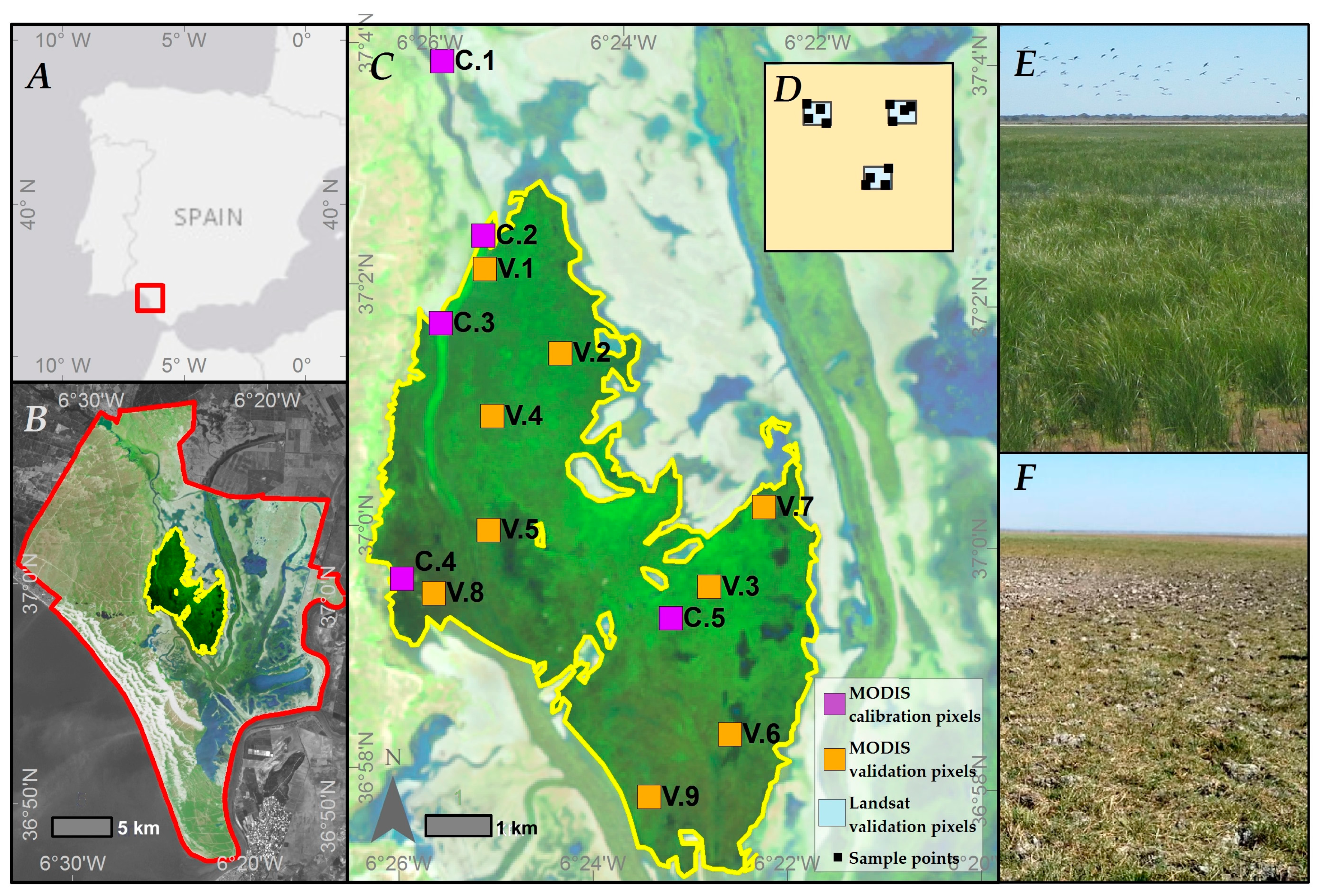
2.1. Study Area
2.2. Satellite Data
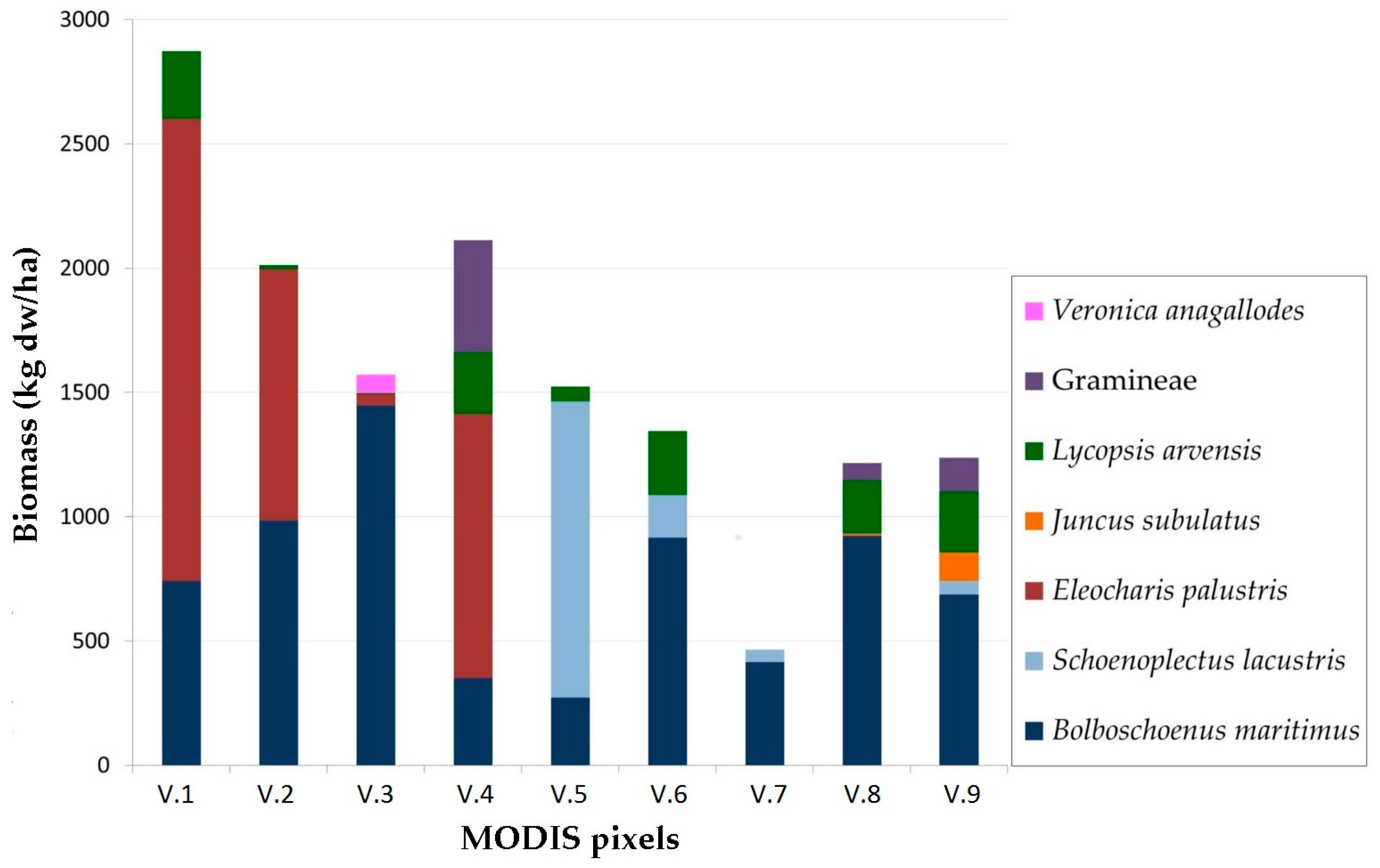
2.3. Biomass Data
2.4. Environmental Data
2.5. Biomass Production Models
- The maximum NDVI value observed in each given year and MODIS pixel (‘Maximum-NDVI’ hereafter).
- The NDVI value at the time at which peak biomass occurs in an average year (8 May), for each given year and MODIS pixel (“May-NDVI” hereafter). The average time of the biomass peak was calculated as the mean date of the maximum NDVI values observed at the five MODIS pixels included in the calibration dataset from 2001 to 2015.
- The maximum and small integral NDVI values derived from phenological models fitted using the Land Surface Phenology (LSP) techniques available in the software package TIMESAT [48] (“LSP-Maximum-NDVI” and “LSP-Accumulated-NDVI” hereafter). The model was fit to the complete series of observed NDVI data (2001–2015) and then compared to the calibration data. The calibration procedure was also used to inform the choice of three settings that must be decided by the user before fitting the curves to NDVI data [49], namely: (1) The baseline value of the phenological curve, a parameter that discards all the values below a specific NDVI value from the growth season under analysis. (2) The criterion that defines the beginning and end of the growth season. We evaluated two options: a fixed threshold value and a fixed proportion of the seasonal amplitude observed during each growth season. (3) The fitting method used to filter noise in the data: Savitzky-Golay filter, Asymmetric Gaussian and Double Logistic. For all other settings, we used the default values in TIMESAT, namely: no spike method, one season per year, no adaptation to the upper envelope of the curve, and normal adaptation strength.
2.6. Model Validation
2.7. Trend Analysis
3. Results
3.1. Biomass Production Models
3.1.1. Model Parametrization
- Baseline value: The best results were obtained with a baseline value of 0.27, which corresponds to the average value of NDVI in September across the whole study area—i.e., the NDVI value of senescent B. maritimus vegetation on dry marsh soil. This baseline value resulted in a much better regression fit than using no fixed baseline value (R2 = 0.63 vs. R2 = 0.22, in the best-performing model and filter: LSP-Accumulated-NDVI with Savitzky-Golay, see below). Other baseline values, like the NDVI value of open water (NDVI = 0.31), resulted in the failure to recognize the growing season—probably because it results in large variations in baseline values between early- and late-flooding years, which is unrelated with plant primary production.
- Beginning and end of the growth season: The criterion based on a proportion of the seasonal amplitude performed better than the one based on a fixed threshold value, which resulted in TIMESAT failing to recognize the growth season for most of the years, due to their strong inter-annual variability. Among the different threshold-amplitude values tested, a value of 10% performed best (R2 = 0.65, as compared to R2 = 0.63 for 3% and R2 = 0.61 for 5%, in the best-performing model and filter: LSP-Maximum-NDVI with Savitzky-Golay, see below), allowing for the recognition of the growth season of all years and succeeding with the filtering of the noise.
- Fitting method: The metrics derived from the Savitzky-Golay filter performed slightly better than those obtained with the other two methods (Table 1). Hence, we solely use and report this method hereafter.
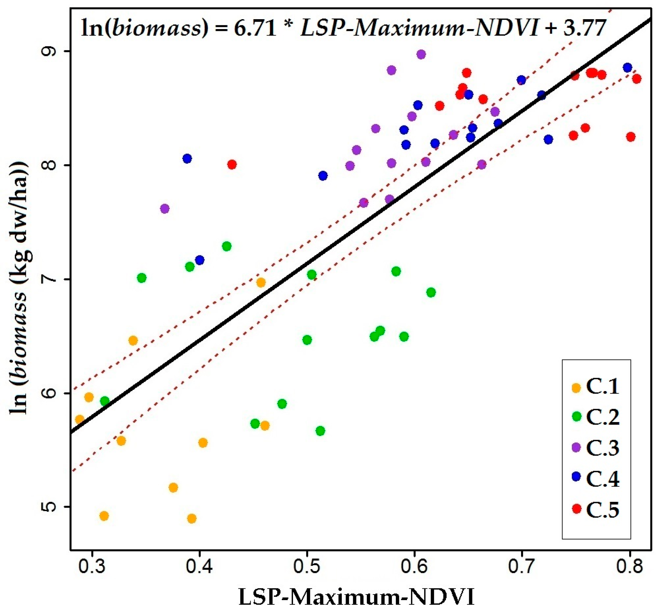
3.1.2. Model Calibration
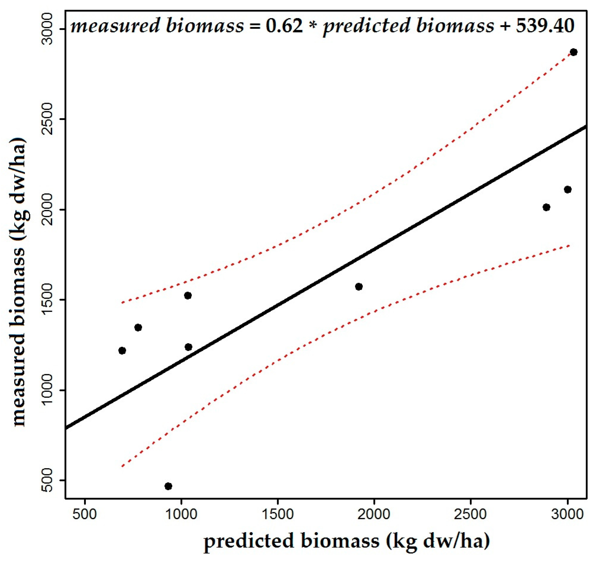
3.2. Model Validation
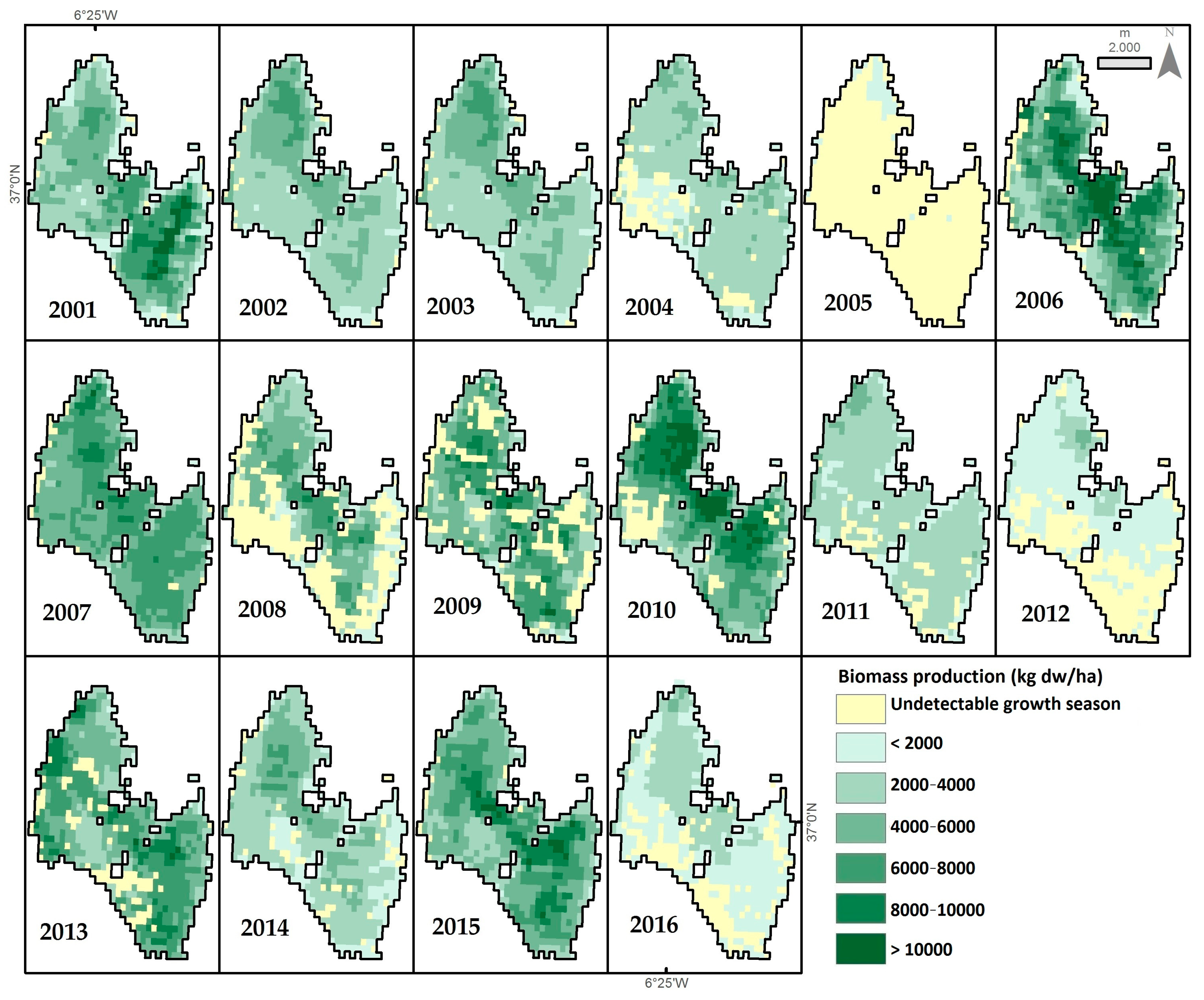
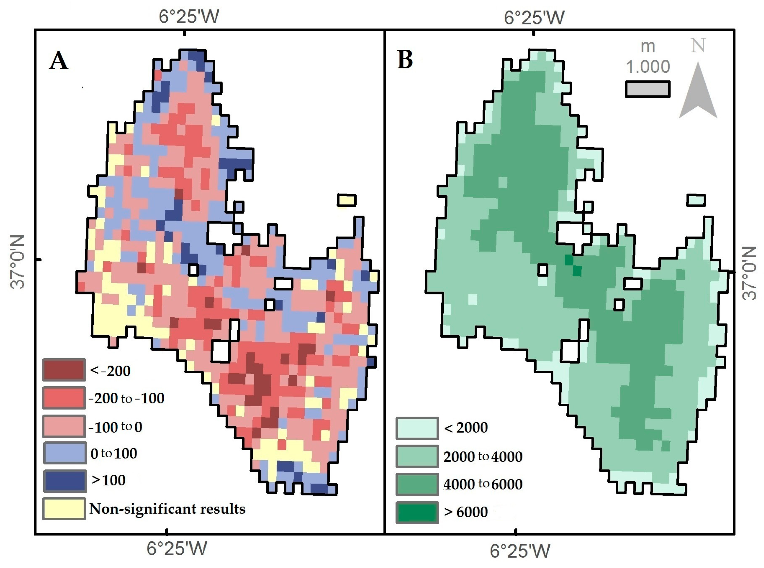
3.3. Trend Analysis
4. Discussion
5. Conclusions
Acknowledgments
Author Contributions
Conflicts of Interest
Appendix A

| Predictor | Intercept ± SE | Slope ± SE | F-Test | DF | p-Value | R2 | RMSE | %RMSE | |
|---|---|---|---|---|---|---|---|---|---|
| y = a * x + b | Maximum-NDVI | −1270 ± 783 | 7023 ± 1267 | 30.7 | 1, 73 | 4.52 × 10⁻⁷ | 0.29 | 1919 | 66.5 |
| May-NDVI | −1104 ± 718 | 7348 ± 1259 | 34.7 | 1, 73 | 1.36 × 10⁻⁷ | 0.32 | 1888 | 65.5 | |
| LSP-Maximum-NDVI | −3641 ± 629 | 12 085 ± 1110 | 118.5 | 1, 69 | < 2.2 × 10⁻¹⁶ | 0.63 | 1400 | 48.6 | |
| LSP-Accumulated-NDVI | 21 ± 327 | 1400 ± 133 | 110.7 | 1, 69 | 5.49 × 10⁻¹⁶ | 0.61 | 1430 | 49.6 | |
| ln (y) = a * ln (x) + b | Maximum-NDVI | 8.26 ± 0.18 | 1.36 ± 0.21 | 39.6 | 1, 73 | 2.09 × 10⁻⁸ | 0.35 | 1.01 | 13.5 |
| May-NDVI | 8.85 ± 0.22 | 2.11 ± 0.28 | 55.8 | 1, 73 | 1.40 × 10⁻¹⁰ | 0.43 | 0.94 | 12.7 | |
| LSP-Maximum-NDVI | 9.60 ± 0.21 | 3.31 ± 0.29 | 133.5 | 1, 68 | < 2.2 × 10⁻¹⁶ | 0.64 | 0.74 | 10.0 | |
| LSP-Accumulated-NDVI | 6.89 ± 0.11 | 1.18 ± 0.11 | 109 | 1, 69 | 7.68 × 10⁻¹⁶ | 0.61 | 0.79 | 10.6 |
References
- Cho, M.A.; Skidmore, A.; Corsi, F.; van Wieren, S.E.; Sobhan, I. Estimation of green grass/herb biomass from airborne hyperspectral imagery using spectral indices and partial least squares regression. Int. J. Appl. Earth Obs. Geoinf. 2007, 9, 414–424. [Google Scholar] [CrossRef]
- Fava, F.; Colombo, R.; Bocchi, S.; Meroni, M.; Sitzia, M.; Fois, N.; Zucca, C. Identification of hyperspectral vegetation indices for Mediterranean pasture characterization. Int. J. Appl. Earth Obs. Geoinf. 2009, 11, 233–243. [Google Scholar] [CrossRef]
- Xiaoping, W.; Ni, G.; Kai, Z.; Jing, W. Hyperspectral remote sensing estimation models of aboveground biomass in Gannan rangelands. Procedia Environ. Sci. 2011, 10, 697–702. [Google Scholar] [CrossRef]
- Moeckel, T.; Safari, H.; Reddersen, B.; Fricke, T.; Wachendorf, M. Fusion of ultrasonic and spectral sensor data for improving the estimation of biomass in grasslands with heterogeneous sward structure. Remote Sens. 2017, 9, 98. [Google Scholar] [CrossRef]
- Carmona, C.P.; Röder, A.; Azcárate, F.M.; Peco, B. Grazing management or physiography? Factors controlling vegetation recovery in Mediterranean grasslands. Ecol. Model. 2013, 251, 73–84. [Google Scholar] [CrossRef]
- Adam, E.; Mutanga, O.; Rugege, D. Multispectral and hyperspectral remote sensing for identification and mapping of wetland vegetation: A review. Wetl. Ecol. Manag. 2010, 18, 281–296. [Google Scholar] [CrossRef]
- Pettorelli, N.; Vik, J.O.; Mysterud, A.; Gaillard, J.M.; Tucker, C.J.; Stenseth, N.C. Using the satellite-derived NDVI to assess ecological responses to environmental change. Trends Ecol. Evol. 2005, 20, 503–510. [Google Scholar] [CrossRef] [PubMed]
- Tiner, R.W.; Lang, M.W.; Klemas, V.V. Remote Sensing of Wetlands: Applications and Advances; CRC Press: Abingdon, UK, 2015. [Google Scholar]
- Yan, E.; Wang, G.; Lin, H.; Xia, C.; Sun, H. Phenology-based classification of vegetation cover types in Northeast China using MODIS NDVI and EVI time series. Int. J. Remote Sens. 2015, 36, 489–512. [Google Scholar] [CrossRef]
- Meroni, M.; Verstraete, M.M.; Rembold, F.; Urbano, F.; Kayitakire, F. A phenology-based method to derive biomass production anomalies for food security monitoring in the Horn of Africa. Int. J. Remote Sens. 2014, 35, 2472–2492. [Google Scholar] [CrossRef]
- Diaz-Delgado, R.; Aragonés, D.; Ameztoy, I.; Bustamante, J. Monitoring marsh dynamics through remote sensing. In Conservation Monitoring in Freshwater Habitats: A Practical Guide and Case Studies; Springer: Berlin, Germany, 2010; pp. 1–415. [Google Scholar]
- Reed, B.C.; Schuwartz, M.D.; Xiao, X. Remote sensing phenology: Status and the way forward. In Phenology of Ecosystems Processes; Springer: Berlin, Germany, 2009; pp. 231–246. [Google Scholar]
- Engman, E.; Gurney, R. Remote Sensing in Hydrology; Springer: Berlin, Germany, 1991. [Google Scholar]
- Díaz-Delgado, R.; Aragonés, D.; Afán, I.; Bustamante, J. Long-term monitoring of the flooding regime and hydroperiod of Doñana marshes with Landsat time series (1974–2014). Remote Sens. 2016, 8, 775. [Google Scholar] [CrossRef]
- Vanderpost, C.; Ringrose, S.; Matheson, W.; Arntzen, J. Satellite based long-term assessment of rangeland condition in semi-arid areas: An example from Botswana. J. Arid Environ. 2011, 75, 383–389. [Google Scholar] [CrossRef]
- Yengoh, G.T.; Dent, D.; Olsson, L.; Tengberg, A.E.; Tucker, C.J., III. Use of the Normalized Difference Vegetation Index (NDVI) to Assess Land Degradation at Multiple Scales: Current Status, Future Trends, and Practical Considerations; Springer: Berlin, Germany, 2015. [Google Scholar]
- Santin-Janin, H.; Garel, M.; Chapuis, J.L.; Pontier, D. Assessing the performance of NDVI as a proxy for plant biomass using non-linear models: A case study on the kerguelen archipelago. Polar Biol. 2009, 32, 861–871. [Google Scholar] [CrossRef]
- Huete, A.; Didan, K.; Miura, T.; Rodriguez, E.P.; Gao, X.; Ferreira, L.G. Overview of the radiometric and biophysical performance of the MODIS vegetation indices. Remote Sens. Environ. 2002, 83, 195–213. [Google Scholar] [CrossRef]
- Lhermitte, S.; Verbesselt, J.; Verstraeten, W.W.; Coppin, P. A comparison of time series similarity measures for classification and change detection of ecosystem dynamics. Remote Sens. Environ. 2011, 115, 3129–3152. [Google Scholar] [CrossRef]
- Meroni, M.; Rembold, F.; Verstraete, M.; Gommes, R.; Schucknecht, A.; Beye, G. Investigating the relationship between the inter-annual variability of satellite-derived vegetation phenology and a proxy of biomass production in the Sahel. Remote Sens. 2014, 6, 5868–5884. [Google Scholar] [CrossRef]
- Lara, B.; Gandini, M. Assessing the performance of smoothing functions to estimate land surface phenology on temperate grassland. Int. J. Remote Sens. 2016, 37, 1801–1813. [Google Scholar] [CrossRef]
- Rojas, O.; Vrieling, A.; Rembold, F. Assessing drought probability for agricultural areas in Africa with coarse resolution remote sensing imagery. Remote Sens. Environ. 2011, 115, 343–352. [Google Scholar] [CrossRef]
- Richardson, A.D.; Black, T.A.; Ciais, P.; Delbart, N.; Friedl, M.A.; Gobron, N.; Hollinger, D.Y.; Kutsch, W.L.; Longdoz, B.; Luyssaert, S.; et al. Influence of spring and autumn phenological transitions on forest ecosystem productivity. Philos. Trans. R. Soc. B Biol. Sci. 2010, 365, 3227–3246. [Google Scholar] [CrossRef] [PubMed]
- Higgins, S.I.; Scheiter, S. Atmospheric CO2 forces abrupt vegetation shifts locally, but not globally. Nature 2012, 488, 209–212. [Google Scholar] [CrossRef] [PubMed]
- Wright, S.J.; van Schaik, C.P. Light and the phenology of tropical trees. Am. Nat. 1994, 143, 192–199. [Google Scholar] [CrossRef]
- Vanschaik, C.P.; Terborgh, J.W.; Wright, S.J. The phenology of tropical forests—Adaptive significance and consequences for primary consumers. Annu. Rev. Ecol. Syst. 1993, 24, 353–377. [Google Scholar] [CrossRef]
- Wolkovich, E.M.; Cook, B.I.; Allen, J.M.; Crimmins, T.M.; Betancourt, J.L.; Travers, S.E.; Pau, S.; Regetz, J.; Davies, T.J.; Kraft, N.J.B.; et al. Warming experiments underpredict plant phenological responses to climate change. Nature 2012, 485, 18–21. [Google Scholar] [CrossRef] [PubMed]
- Adole, T.; Dash, J.; Atkinson, P.M. A systematic review of vegetation phenology in Africa. Ecol. Inform. 2016, 34, 117–128. [Google Scholar] [CrossRef]
- Hanes, J.M. Biophysical Applications of Satellite Remote Sensing; Springer: Berlin, Germany, 2014. [Google Scholar]
- Huete, A.; Didan, K.; van Leeuwen, W.; Miura, T.; Glenn, E. MODIS vegetation indices. Remote Sens. Digit. Image Process. 2011, 11, 579–602. [Google Scholar]
- Boyd, D.S.; Almond, S.; Dash, J.; Curran, P.J.; Hill, R.A.; Hill, R.A. Phenology of vegetation in southern England from Envisat MERIS terrestrial chlorophyll index (MTCI) data. Int. J. Remote Sens. 2011, 3223, 8421–8447. [Google Scholar] [CrossRef]
- Zucca, C.; Wu, W.; Dessena, L.; Mulas, M. Assessing the effectiveness of land restoration interventions in dry lands by multitemporal remote sensing—A case study in Ouled DLIM (Marrakech, Morocco). Land Degrad. Dev. 2015, 26, 80–91. [Google Scholar] [CrossRef]
- Moulin, S.; Guérif, M. Impacts of model parameter uncertainties on crop reflectance estimates: A regional case study on wheat. Int. J. Remote Sens. 1999, 20, 213–218. [Google Scholar] [CrossRef]
- Huete, A.R. A soil-adjusted vegetation index (SAVI). Remote Sens. Environ. 1988, 25, 295–309. [Google Scholar] [CrossRef]
- Box, E.O.; Holben, B.N.; Kalb, V. Accuracy of the AVHRR vegetation index as a predictor of biomass, primary productivity and net CO2 flux. Vegetatio 1989, 80, 71–89. [Google Scholar] [CrossRef]
- Eisfelder, C.; Kuenzer, C.; Dech, S. Derivation of biomass information for semi-arid areas using remote-sensing data. Int. J. Remote Sens. 2012, 33, 2937–2984. [Google Scholar] [CrossRef]
- Mbow, C.; Fensholt, R.; Rasmussen, K.; Diop, D. Can vegetation productivity be derived from greenness in a semi-arid environment? Evidence from ground-based measurements. J. Arid Environ. 2013, 97, 56–65. [Google Scholar] [CrossRef]
- Gallant, A.L. The challenges of remote monitoring of wetlands. Remote Sens. 2015, 7, 10938–10950. [Google Scholar] [CrossRef]
- Röder, A.; Udelhoven, T.; Hill, J.; del Barrio, G.; Tsiourlis, G. Trend analysis of Landsat-TM and -ETM+ imagery to monitor grazing impact in a rangeland ecosystem in Northern Greece. Remote Sens. Environ. 2008, 112, 2863–2875. [Google Scholar] [CrossRef]
- Soriguer, R.C.; Rodriguez Sierra, A.; Domínquez Nevado, L. Análisis de la Incidencia de los Grandes Herbívoros en la Marisma y Vera del Parque Nacional de Doñana; Organismo Autónomo de Parques Nacionales: Segovia, Spain, 2001. [Google Scholar]
- Soriguer, R.C. Consideraciones sobre el efecto de los conejos y los grandes herbívoros en los pastizales de la Vera de Doñana. Doñana Acta Vertebr. 1983, 10, 155–168. [Google Scholar]
- Clemente, L.; García, L.-V.; Espinar, J.L.; Cara, J.S.; Moreno, A. Las marismas del Parque Nacional de Doñana. Investig. Cienc. 2004, 332, 72–83. [Google Scholar]
- Castroviejo, J. Memoria Mapa del Parque Nacional de Doñana; Consejo Superior de Investigaciones Científicas: Madrid, Spain, 1993. [Google Scholar]
- Figuerola, J.; Green, A.J.; Santamaría, L. Passive internal transport of aquatic organisms by waterfowl in Doñana, south-west Spain. Glob. Ecol. Biogeogr. 2003, 12, 427–436. [Google Scholar] [CrossRef]
- Aragonés, D.; Díaz-Delgado, R.; Bustamante, J. Estudio de la dinámica de inundación histórica de las marismas de Doñana a partir de una serie temporal larga de imágenes Landsat. Procceedings of XI Congreso Nacional de Teledetección, Pto. de la Cruz, Spain, 14 September 2005. [Google Scholar]
- Vuolo, F.; Mattiuzzi, M.; Klisch, A.; Atzberger, C. Data service platform for MODIS Vegetation Indices time series processing at BOKU Vienna: Current status and future perspectives. Procceedings of SPIE Remote Sensing, Edinburgh, UK, 24–27 September 2012. [Google Scholar]
- Huete, A.R.; Didan, K.; Huete, A.; Didan, K.; Van Leeuwen, W.; Jacobson, A.; Solanos, R.; Laing, T. MODIS Vegetation Index (MOD 13) Algorithm Theoretical Basis Document; Vegetation Index and Phenology Lab: Tucson, AZ, USA, 1999. [Google Scholar]
- Jonsson, P.; Eklundh, L. TIMESAT—A program for analyzing time-series of satellite sensor data. Comput. Geosci. 2004, 30, 833–845. [Google Scholar] [CrossRef]
- Eklundh, L.; Jönsson, P. TIMESAT 3.2 with Parallel Processing Software Manual; Lund University: Lund, Sweden, 2015. [Google Scholar]
- Fox, J.; Weisberg, S. An R Companion to Applied Regression; SAGE Publication: Thousand Oaks, CA, USA, 2011. [Google Scholar]
- Legendre, P. Model II Regression User's Guide, R Edition; Département de sciences biologiques, Univ. de Montreal: Quebec, QC, Canada, 2014. [Google Scholar]
- R Core Team. R: A Language and Environment for Statistical Computing; R Foundation for Statistical Computing: Vienna, Austria, 2013. [Google Scholar]
- Crawley, M.J. The R Book; John Wiley & Sons Inc.: Hoboken, NJ, USA, 2012. [Google Scholar]
- Eastman, J.R. Earth Trends Modeler in Terrset; Clark Labs: Worcester, MA, USA, 2009. [Google Scholar]
- Bustamante, J.; Aragonés, D.; Afán, I. Effect of protection level in the hydroperiod of water bodies on Doñana’s aeolian sands. Remote Sens. 2016, 8, 867. [Google Scholar] [CrossRef]
- Moreau, S.; Bosseno, R.; Gu, X.F.; Baret, F. Assessing the biomass dynamics of Andean bofedal and totora high-protein wetland grasses from NOAA/AVHRR. Remote Sens. Environ. 2003, 85, 516–529. [Google Scholar] [CrossRef]
- Kang, X.; Hao, Y.; Cui, X.; Chen, H.; Huang, S.; Du, Y.; Li, W.; Kardol, P.; Xiao, X.; Cui, L. Variability and changes in climate, phenology, and gross primary production of an alpine wetland ecosystem. Remote Sens. 2016, 8, 391. [Google Scholar] [CrossRef]
- Hird, J.N.; McDermid, G.J. Noise reduction of NDVI time series: An empirical comparison of selected techniques. Remote Sens. Environ. 2009, 113, 248–258. [Google Scholar] [CrossRef]
- Klemas, V. Remote sensing of coastal and ocean currents: An overview. J. Coast. Res. 2012, 282, 576–586. [Google Scholar] [CrossRef]
- Villa, P.; Mousivand, A.; Bresciani, M. Aquatic vegetation indices assessment through radiative transfer modeling and linear mixture simulation. Int. J. Appl. Earth Obs. Geoinf. 2014, 30, 113–127. [Google Scholar] [CrossRef]
- Stephens, P.A.; Pettorelli, N.; Barlow, J.; Whittingham, M.J.; Cadotte, M.W. Management by proxy? The use of indices in applied ecology. J. Appl. Ecol. 2015, 52, 1–6. [Google Scholar] [CrossRef]
- García-Murillo, P.; Bazo, E.; Fernández-Zamudio, R. Las plantas de la marisma del Parque Nacional de Doñana (España): Elemento clave para la conservación de un humedal europeo paradigmático. CienciaUAT 2014, 9, 60–75. [Google Scholar]
- Coe, M.J.; Cumming, D.H.; Phillipson, G. Biomass and production of large african herbivores in relation to rainfall and primary production. Oecologia 1976, 22, 341–354. [Google Scholar] [CrossRef] [PubMed]
- Li, Z.; Huffman, T.; McConkey, B.; Townley-Smith, L. Monitoring and modeling spatial and temporal patterns of grassland dynamics using time-series MODIS NDVI with climate and stocking data. Remote Sens. Environ. 2013, 138, 232–244. [Google Scholar] [CrossRef]
- Archer, E.R.M. Beyond the “climate versus grazing” impasse: Using remote sensing to investigate the effects of grazing system choice on vegetation cover in the eastern Karoo. J. Arid Environ. 2004, 57, 381–408. [Google Scholar] [CrossRef]
- Li, A.; Wu, J.; Huang, J. Distinguishing between human-induced and climate-driven vegetation changes: A critical application of RESTREND in inner Mongolia. Landsc. Ecol. 2012, 27, 969–982. [Google Scholar] [CrossRef]
- Hooke, J.; Sandercock, P. Use of vegetation to combat desertification and land degradation: Recommendations and guidelines for spatial strategies in Mediterranean lands. Landsc. Urban Plan. 2012, 107, 389–400. [Google Scholar] [CrossRef]


| Asymmetrical Gaussian | Double Logistic | Savitzky-Golay | |
|---|---|---|---|
| LSP-Maximum-NDVI | 0.60 | 0.62 | 0.63 |
| LSP-Accumulated-NDVI | 0.53 | 0.54 | 0.61 |
| Predictor | Intercept ± SE | Slope ± SE | F-Test | DF | p-Value | R2 | RMSE | %RMSE |
|---|---|---|---|---|---|---|---|---|
| Maximum-NDVI | 4.75 ± 0.39 | 4.51 ± 0.63 | 51 | 1, 73 | 5.71 × 10⁻¹⁰ | 0.41 | 0.96 | 12.9 |
| May-NDVI | 5.00 ± 0.70 | 4.46 ± 0.65 | 47.3 | 1, 73 | 1.76 × 10⁻⁹ | 0.39 | 0.97 | 13.1 |
| LSP-Maximum-NDVI | 3.77 ± 0.34 | 6.71 ± 0.59 | 128 | 1, 69 | < 2.2 × 10⁻¹⁶ | 0.65 | 0.74 | 10.1 |
| LSP-Accumulated-NDVI | 5.88 ± 0.19 | 0.75 ± 0.08 | 97 | 1, 69 | 8.1 × 10⁻¹⁵ | 0.59 | 0.81 | 11.0 |
| Predictors | Estimates ± SE | T-test | p-Values | Whole-model Parameters | ||||||
|---|---|---|---|---|---|---|---|---|---|---|
| F-test | DF | p-Value | Adj. R2 | RMSE | %RMSE | |||||
| Intercept | 3.69 ± 0.41 | 9.01 | 2.4 × 10⁻¹⁶ | 63.6 | 2, 68 | 2.7 × 10⁻¹⁶ | 0.64 | 0.75 | 10.1 | |
| LSP-Maximum-NDVI | 6.61 ± 0.63 | 10.4 | 9.9 × 10⁻¹⁶ | |||||||
| Precipitation | 2.8 ± 6.3 × 10⁻⁴ | 0.45 | 0.66 | |||||||
| Intercept | 3.73 ± 0.34 | 10.8 | 5.0 × 10⁻¹⁶ | 63.0 | 2, 63 | 9.3 × 10⁻¹⁶ | 0.66 | 0.74 | 10.0 | |
| LSP-Maximum-NDVI | 6.73 ± 0.64 | 10.5 | 1.7 × 10⁻¹⁵ | |||||||
| Hydroperiod 1 | 6.3 ± 14 × 10−4 | 0.46 | 0.65 | |||||||
| Intercept | 6.98 ± 0.45 | 15.2 | < 2.2 × 10⁻¹⁶ | 4.1 | 9, 61 | < 2.2 × 10⁻¹⁶ | 0.85 | 0.46 | 6.2 | |
| Location | DV1 | −1.59 ± 0.22 | −6.69 | 1.98 × 10⁻⁹ | ||||||
| DV2 | −0.11 ± 0.19 | −0.60 | 0.55 | |||||||
| DV3 | −2.17 ± 0.29 | −7.47 | 2.56 × 10⁻¹⁰ | |||||||
| DV4 | −0.09 ± 0.18 | −5.51 | 0.61 | |||||||
| LSP-Maximum-NDVI | 2.26 ± 0.63 | 3.61 | 5.91 × 10⁻⁴ | |||||||
© 2017 by the authors. Licensee MDPI, Basel, Switzerland. This article is an open access article distributed under the terms and conditions of the Creative Commons Attribution (CC BY) license (http://creativecommons.org/licenses/by/4.0/).
Share and Cite
Lumbierres, M.; Méndez, P.F.; Bustamante, J.; Soriguer, R.; Santamaría, L. Modeling Biomass Production in Seasonal Wetlands Using MODIS NDVI Land Surface Phenology. Remote Sens. 2017, 9, 392. https://doi.org/10.3390/rs9040392
Lumbierres M, Méndez PF, Bustamante J, Soriguer R, Santamaría L. Modeling Biomass Production in Seasonal Wetlands Using MODIS NDVI Land Surface Phenology. Remote Sensing. 2017; 9(4):392. https://doi.org/10.3390/rs9040392
Chicago/Turabian StyleLumbierres, Maria, Pablo F. Méndez, Javier Bustamante, Ramón Soriguer, and Luis Santamaría. 2017. "Modeling Biomass Production in Seasonal Wetlands Using MODIS NDVI Land Surface Phenology" Remote Sensing 9, no. 4: 392. https://doi.org/10.3390/rs9040392
APA StyleLumbierres, M., Méndez, P. F., Bustamante, J., Soriguer, R., & Santamaría, L. (2017). Modeling Biomass Production in Seasonal Wetlands Using MODIS NDVI Land Surface Phenology. Remote Sensing, 9(4), 392. https://doi.org/10.3390/rs9040392