1. Introduction
In urban planning, provision of green space (GS) in urban areas is one of the most challenging issues, whereas urban green space (UGS) provides valuable direct and indirect services to the surrounding areas [
1]. For example, Nishinomiya City in Hyogo Prefecture, Japan is promoting improvement and maintenance of its landscapes. It enacted a regulation for one residential area to the effect that newly constructed houses should have a green space ratio (proportion of vegetation to visible area: GSR) of at least 15%. The regulation specifies a simple formula for calculating the green space ratio [
2]. Local governments assess landscape quality from the perspective of aesthetics before approving new construction. The landscape index is calculated through ground surveys by local government officials. However, such surveys are time-consuming and expensive when applied over wide areas, making it difficult to apply the regulation to the entire city and consequently promote more UGS.
Automatic measures of UGS come mainly from geographic information system (GIS) data and remotely sensed data [
3]. For example, Tian et al. [
4] used high-quality digital maps with a spatial resolution of 0.5 m × 0.5 m to analyze the landscape pattern of UGS for ecological quality. Gupta et al. [
5] calculated an urban neighborhood green index to quantify homogenous greenness from multi-temporal satellite images. The periodically obtained remotely sensed imagery is suitable for updating the spatial distribution patterns of GS, but it is limited in that the three-dimensional (3D) distribution is not directly obtained.
As a tool for directly measuring 3D coordinate values, light detection and ranging (LiDAR) measures laser light reflected from the surfaces of objects. The discrete LiDAR data are used to model the 3D surfaces of objects and derive their attributes. Now, airborne and terrestrial LiDAR are of operational use. Terrestrial LiDAR is stationary or mobile by vehicle. Applications of LiDAR data to landscape analysis require the extraction of vegetation via classification and segmentation of point clouds. In the case of airborne LiDAR, vegetation returns the light in various ways—from the surface, middle and bottom—whereas buildings return the light mainly from the surface. This unique feature of multiple returns is a challenge to applying LiDAR data to vegetation extraction. It is well known that the first and last pulses of the light reflected from vegetation correspond to the top (canopies) and bottom (ground) of the vegetation, respectively, which allows the heights of the vegetation surface and ground to be estimated. Thus, we can derive the heights of vegetation by subtracting the ground height from the vegetation surface height. Over the last decade, full-waveform airborne LiDAR has been examined [
6,
7], which can provide more detailed patterns of reflected light and has the potential to estimate the structure of forests.
In a complex urban area, the automatic extraction of vegetation requires the classification of man-made and natural objects. This is another challenge to applying LiDAR data to urban vegetation. One of the most promising approaches is to process the LiDAR data on multiple scales [
8,
9,
10]. For example, Brodu and Lague [
11] presented a method to monitor the local cloud geometry behavior across several scales by changing the diameter of the sphere for representing local features. Wakita and Susaki [
12] proposed a multi-scale and shape-based method to extract vegetation in complex urban areas from terrestrial LiDAR data.
Landscape indices related to GS can be calculated from the vegetation extracted from point clouds or other sources. Susaki and Komiya [
13] proposed a method to estimate the green space ratio (GSR) in urban areas from airborne LiDAR and aerial images intended for the quantitative assessment of local landscapes. The GSR is defined as the ratio of the area occluded by vegetation to the entire visible area at a height of a person on the ground. Following Wakita and Susaki [
12], Wakita et al. [
14] developed a method to estimate GSR from terrestrial LiDAR data. Huang et al. [
15] extracted urban vegetation using point clouds and remote sensing image. Individual tree crowns were extracted using the normalized digital surface model from airborne LiDAR data and the normalized vegetation index (NDVI) from near-infrared image. Yang et al. [
16] estimated Green View index using field survey data and photographs. Yu et al. [
17] presented the Floor Green View Index, an indicator defined as the area of visible vegetation on a particular floor of a building. This index is calculated from airborne LiDAR data and aerial near-infrared photographs to calculate NDVI. Because of occlusion, more accurate extraction of vegetation can be achieved using terrestrial LiDAR data. In addition to terrestrial stationary LiDAR, mobile (or vehicle-based) LiDAR has been examined for this purpose because it is capable of rapidly measuring the data in a large area [
18]. Yang and Dong [
19] proposed a method to segment mobile LiDAR data into objects using shape information derived from the data. However, mobile LiDAR data have a wide range of point density, and thus the estimation of vegetation may tend to be unstable when there is vegetation in the far distance. Therefore, in this research, we present a method to extract vegetation in complex urban areas and estimate a GSR from mobile LiDAR data.
2. Data Used and Study Area
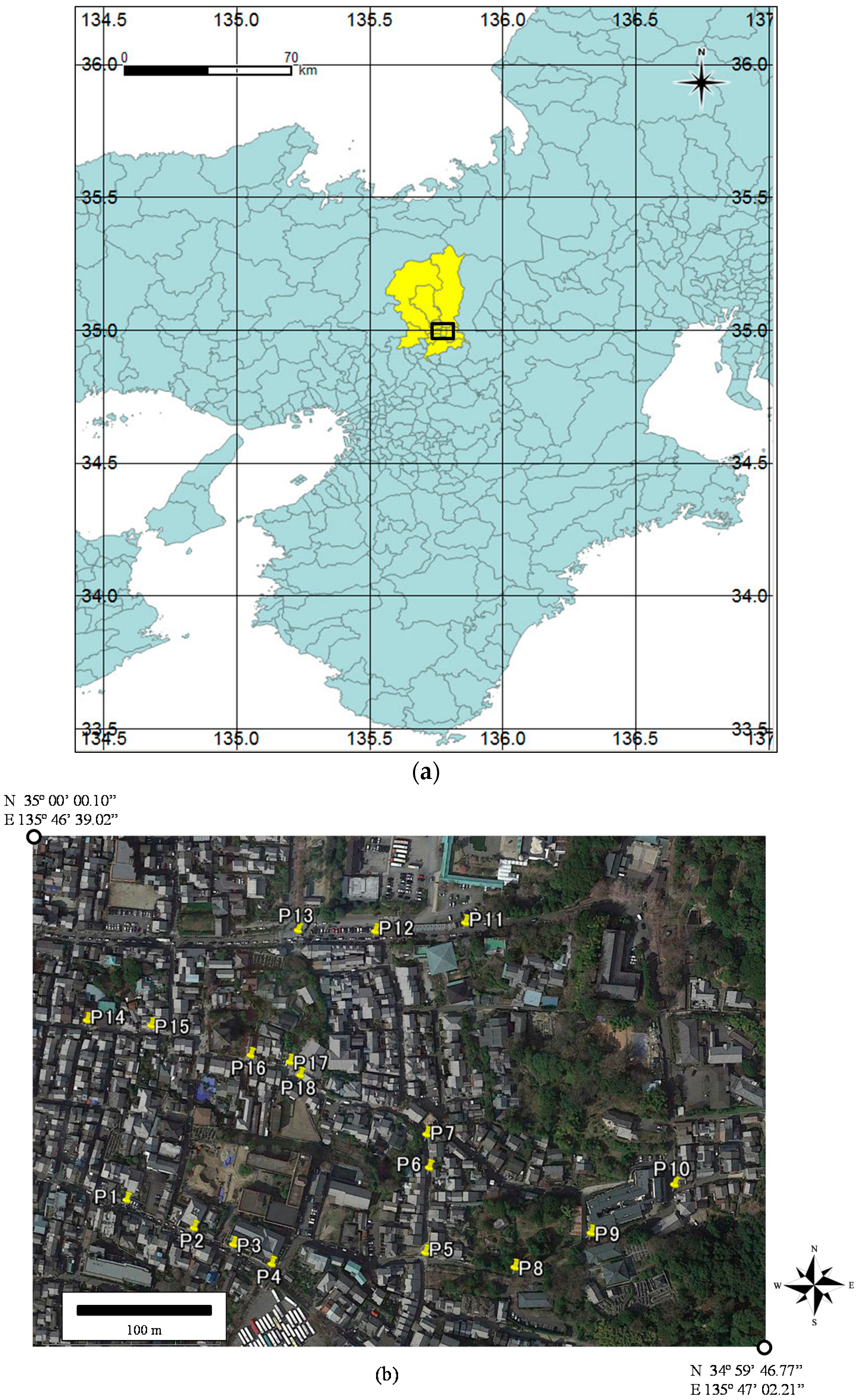
We used a mobile LiDAR system, Trimble MX5, which is a vehicle-mounted LiDAR whose angles were set to 30° for pitch rotation and 0° for heading rotation. The height of LiDAR was set to approximately 2.3 m. It measures 550,000 points per second at a maximum distance of 800 m. The system also has three cameras, which were set to −15°, 0° and 15° for heading rotation. The camera resolution was five million pixels. The measurements were carried out on 3 March 2014 in the Higashiyama Ward of Kyoto, Japan. Higashiyama contains plenty of GS around traditional temples and shrines.
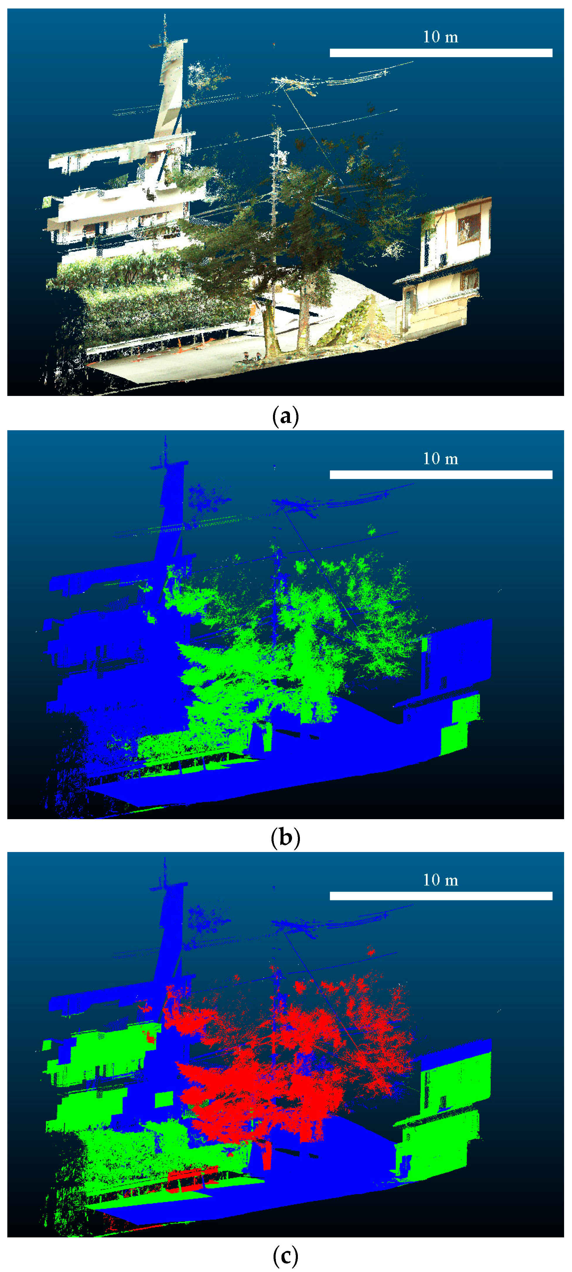
Figure 1 shows the study area.
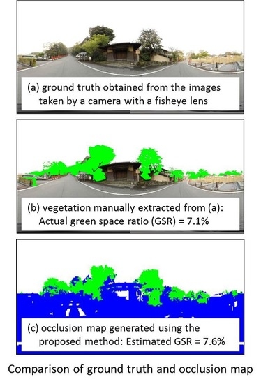
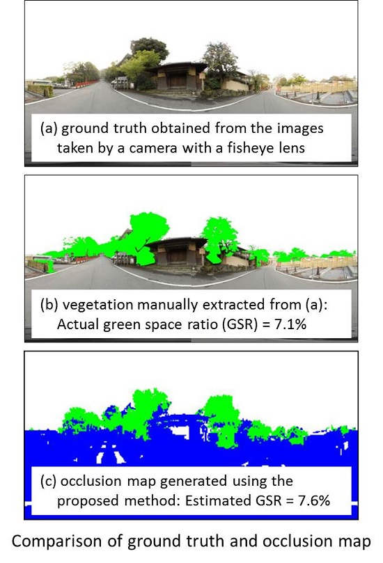
To assess the accuracy of the GSR estimated in this research, we used images taken on 11 April 2015 using a camera with a fisheye lens. Although there was almost a year between the mobile LiDAR and image data, we compared the equivalent color information in the point clouds and the camera images and concluded that the effect of the time gap was not significant. The camera used was an EOS Kiss X3 by Canon, and the fisheye lens was a 4.5-mm F2.8 EX DC Circular Fisheye by Sigma. We selected 18 points as assessment positions, labeled P1 to P18 in
Figure 1. We took two images covering the forward and backward views at each position. We manually colored the vegetation areas and converted two images into one panoramic image, from which we calculated the measured GSR. At each position, we measured actual GSR and estimated GSR from LiDAR data. The measured GSRs were used as the ground truth for validating the estimated GSR results.
3. Green Space Ratio (GSR)
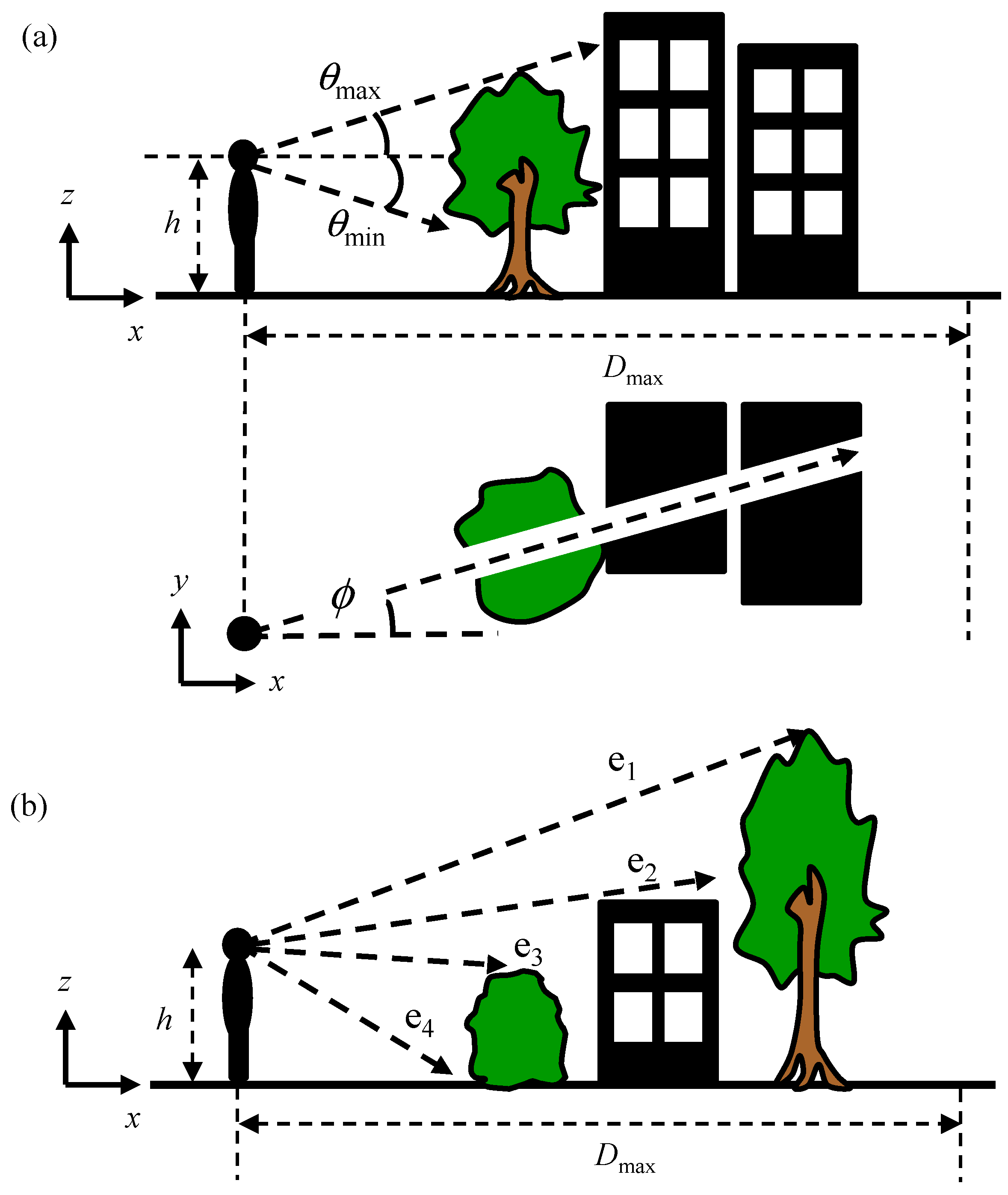
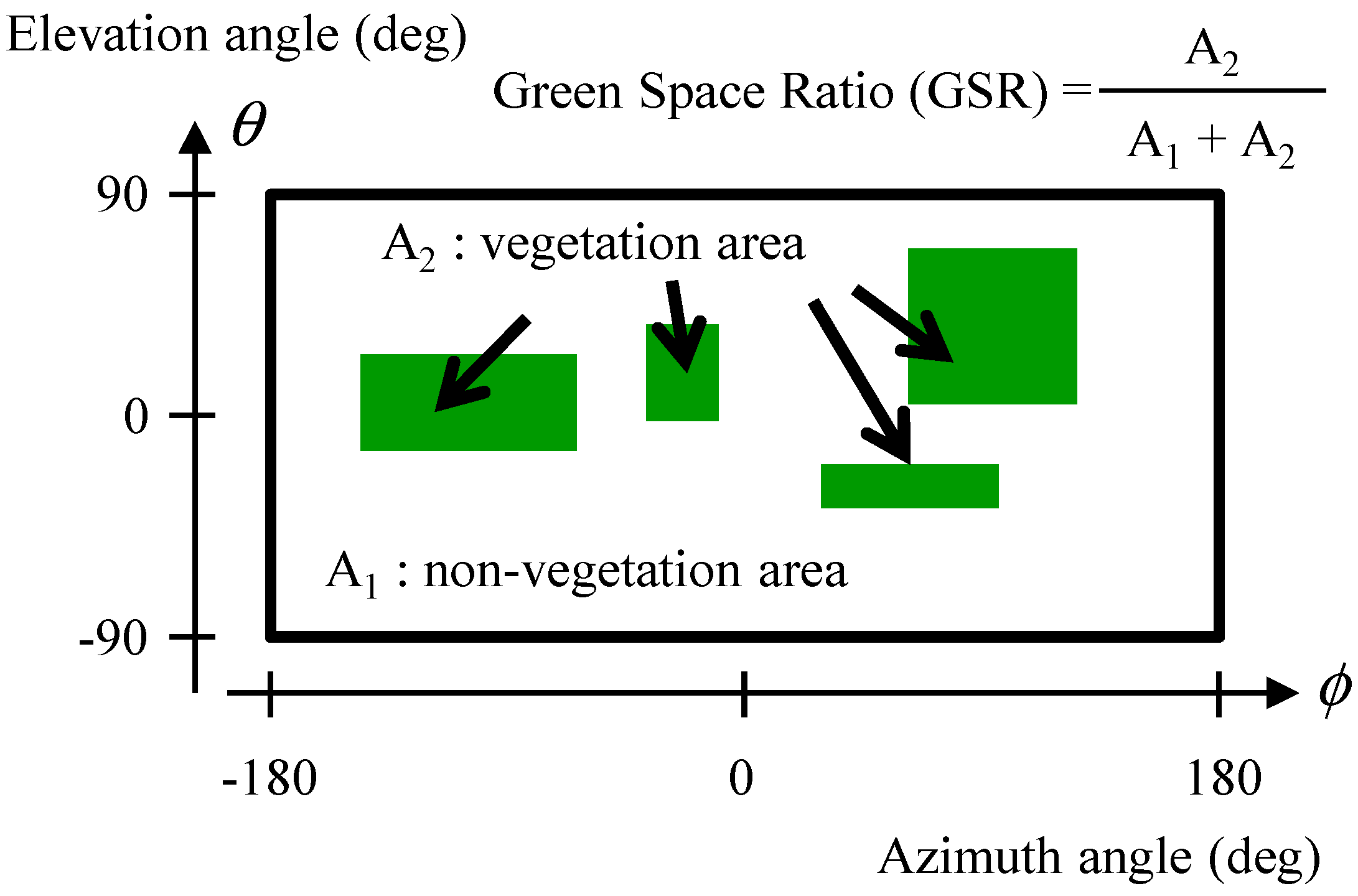
Assume that the vegetation distribution in 3D coordinates is known in advance. We vary the azimuth from 0° to 360° and determine the maximum and minimum elevation angles at which the view is occluded by vegetation.
Figure 2a) shows the viewable area from the perspective of a person facing in the direction of the azimuth
φ. We assume that
φ and the elevation angle
θ are uniformly divided into intervals ∆
φ and ∆
θ, respectively. We vary the value of
φ in steps of ∆
φ from 0° to 360°—∆
φ, and search for vegetation points along each ray at angle
φ within the maximum range
Dmax. At every vegetation point, we can calculate the values of
θ at which occlusion occurs because of vegetation and thereby determine the maximum elevation angle
θmax and the minimum elevation angle
θmin within the maximum range
Dmax (
Figure 2a). If multiple populations of vegetation exist, the maximum and minimum elevation angles occluded by each one are examined (
Figure 2b). As a result, we can generate a map similar to the one shown in
Figure 3 (referred to hereinafter as an occlusion map). The GSR in azimuth–elevation angle space is given by
where
A1 and
A2 denote the non-vegetation area and the occluded vegetation area, respectively, in azimuth–elevation angle space. According to Equation (1), the GSR can take any value between 0% and 100%.
5. Results
We conducted experiments using the data explained in
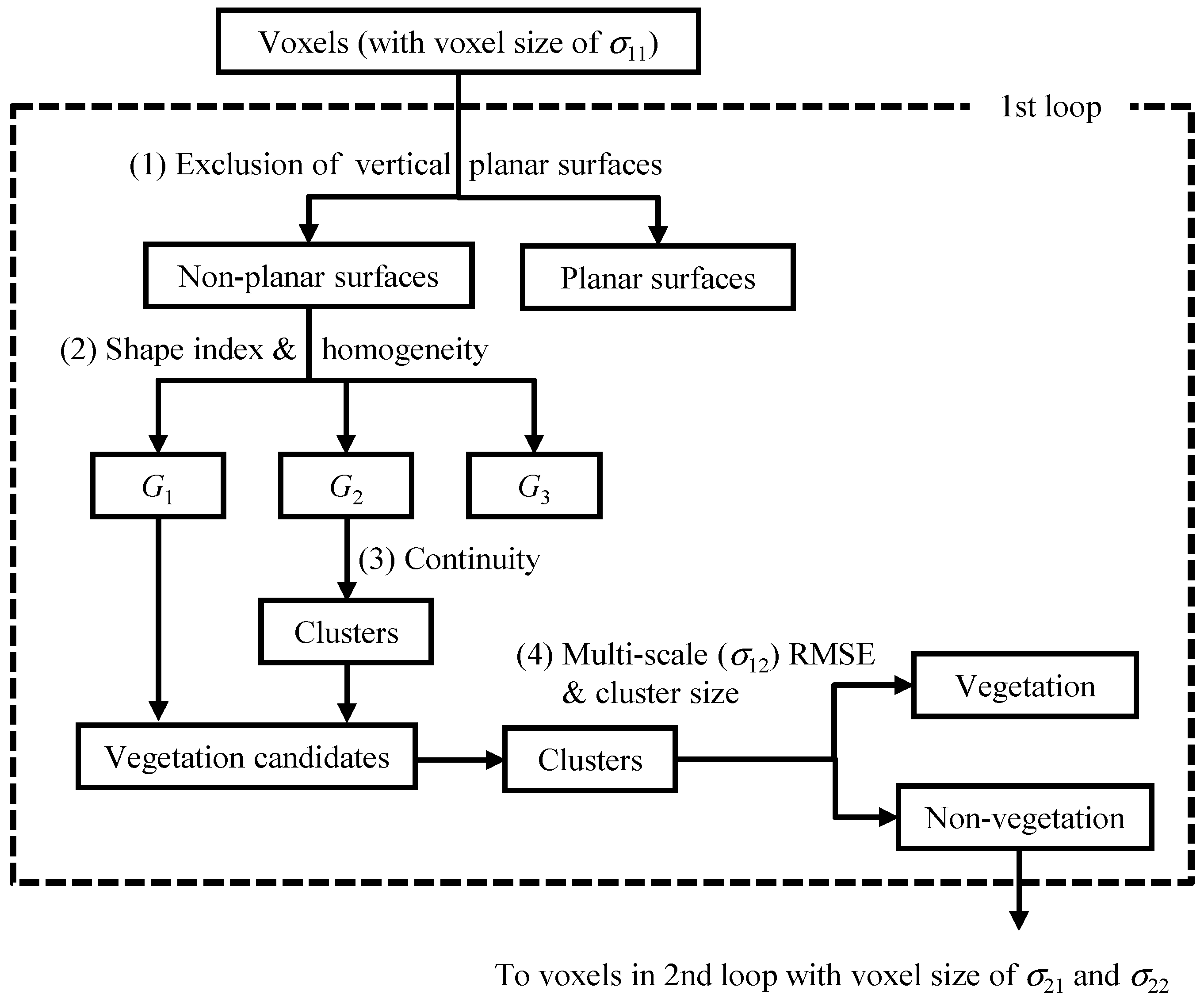
Section 2. We set parameter values required for the proposed method through experiments with sample data as follows. In vegetation extraction, the normal for labeling vertical planar surfaces was defined to have a zenith angle from 85° to 95°. Two sizes of a voxel in the first loop,
σ11 and
σ12, were set to 0.5 m and 1.0 m, respectively. In the second loop,
σ21 and
σ22 were set to 1.0 m and 2.0 m, respectively. The vegetation extraction was repeated with different thresholds. In the first loop,
a11 and
a12 were used as thresholds related to slope
a. In the second loop,
a21 and
a22 were used. We set the thresholds through the experiment with samples as follows:
a11 = 0.02,
a12 = 0.1,
a21 = 0.06, and
a22 = 0.2. The threshold for
homogeneity and
continuity was set to 0.55. Neighboring was defined as a 5 × 5 × 5 voxel space. In noise removal, the number of voxels for a cluster to be labeled as noise was 50 in the first loop and 10 in the second loop. Moreover, if
c1 was greater than 0.6 or
c3 was smaller than 0.05, the cluster was regarded as a noise cluster.
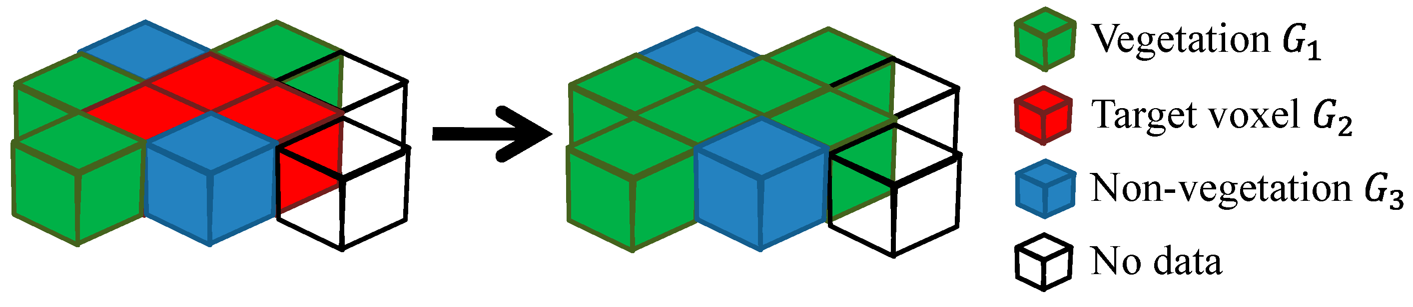
In GSR estimation, the size of a voxel was set to 0.5 m. As for dividing a point cloud into sub-regions, the grid size was 20 m and the overlap length between two adjoining grids was 3 m. The voxel size for storing labeled point clouds was set to 0.5 m. The threshold of Nall for labeling a voxel as no object was set to 2, and the threshold of rv for labeling as non-vegetation, or else as vegetation, was set to 0.5. In estimating the GSR, the height h of a person was set to 1.5 m.
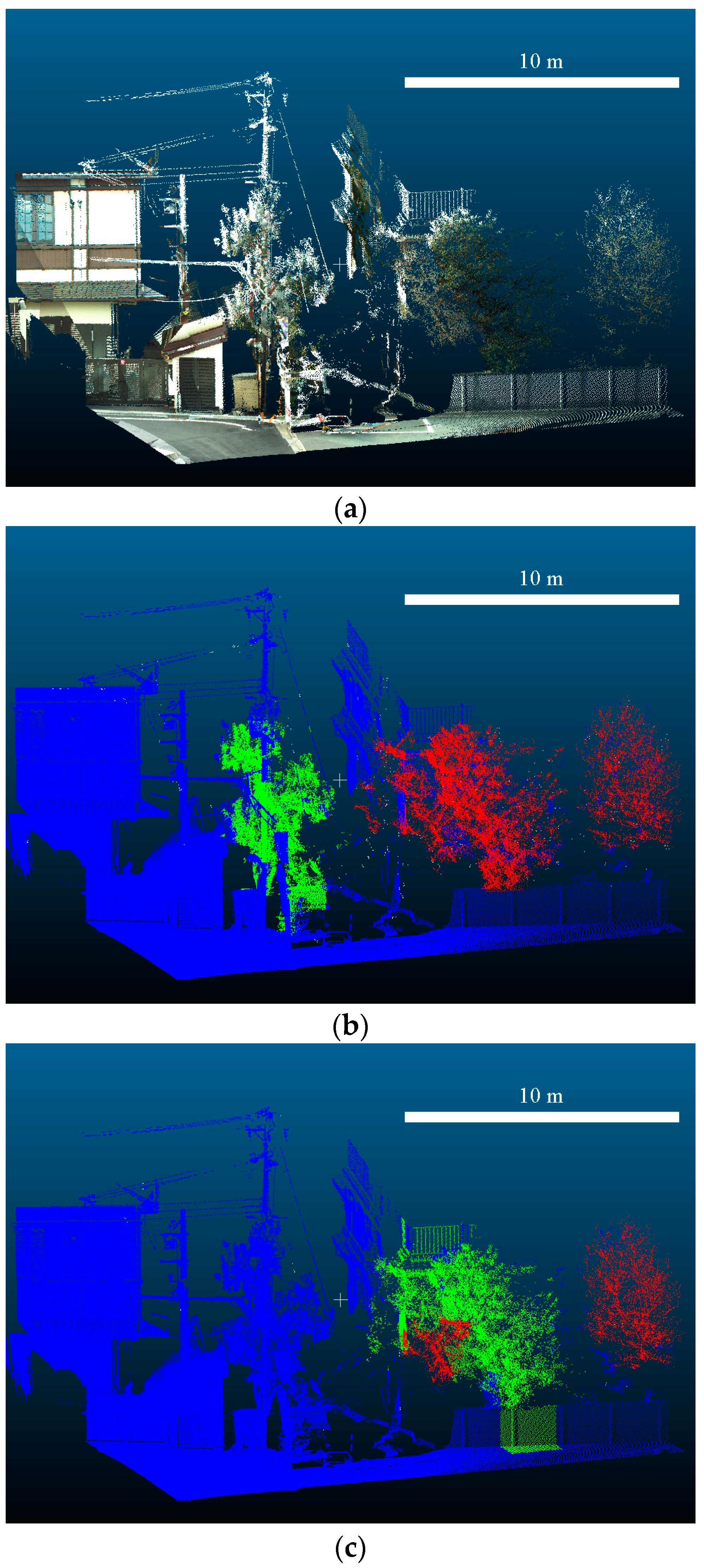
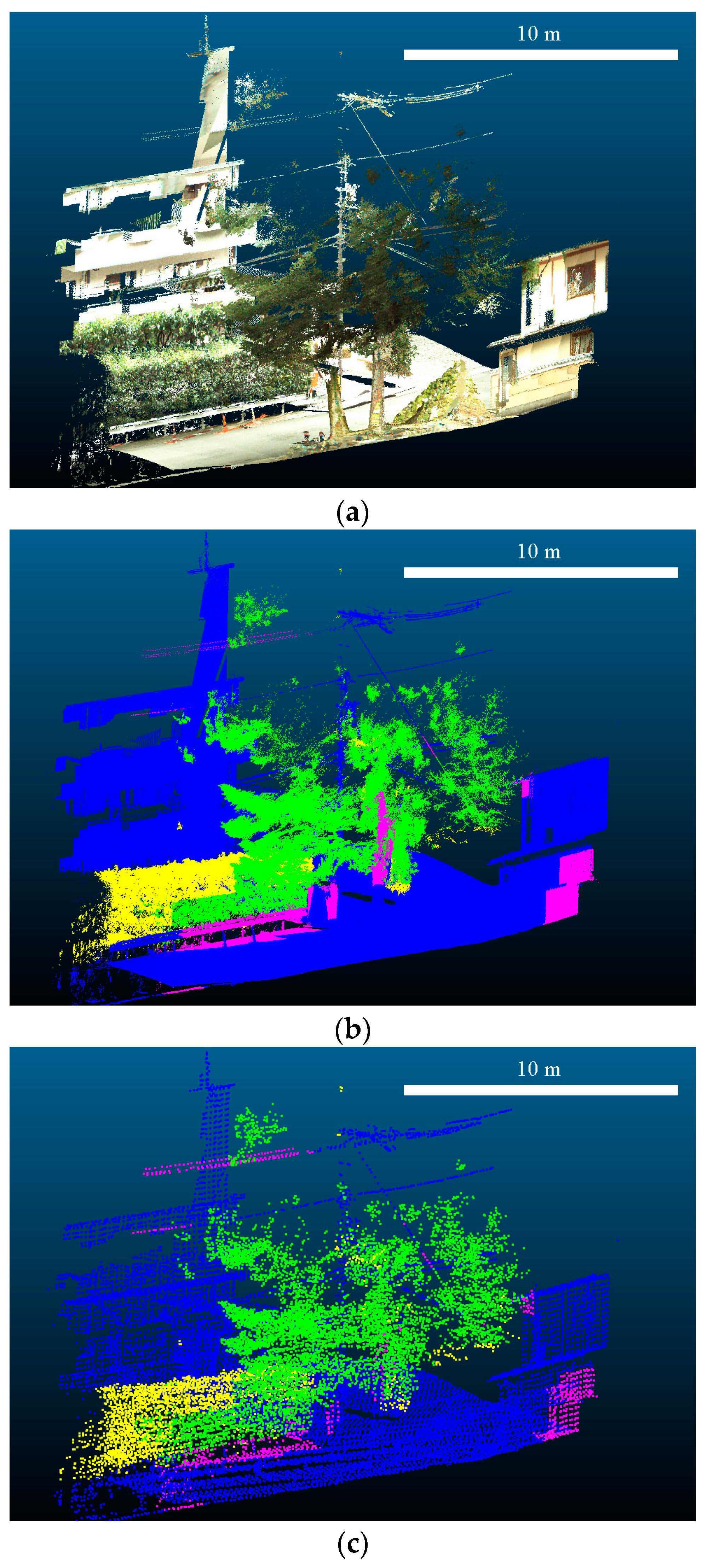
To show the performance of vegetation extraction,
Figure 8 and
Figure 9 demonstrate the improvement of extracting vegetation based on a multi-spatial-scale approach and the effect of the voxel sizes set for the experiments.
Figure 8b and
Figure 9b are the results obtained by applying the optimal parameter values.
We conducted accuracy assessments for vegetation extraction and GSR estimation. The former were assessed by F-measure, as shown in Equation (7):
where,
TP,
TN,
FP and
FN denote true positive, true negative, false positive and false negative, respectively. The results are given in
Table 1.
Figure 10 shows points of the four labels in two cases: using original point clouds and using voxels. Assessment using the original points may be biased because far fewer points were observed around vegetation. Therefore, we assessed the results by aggregating the labels of points into those of voxels.
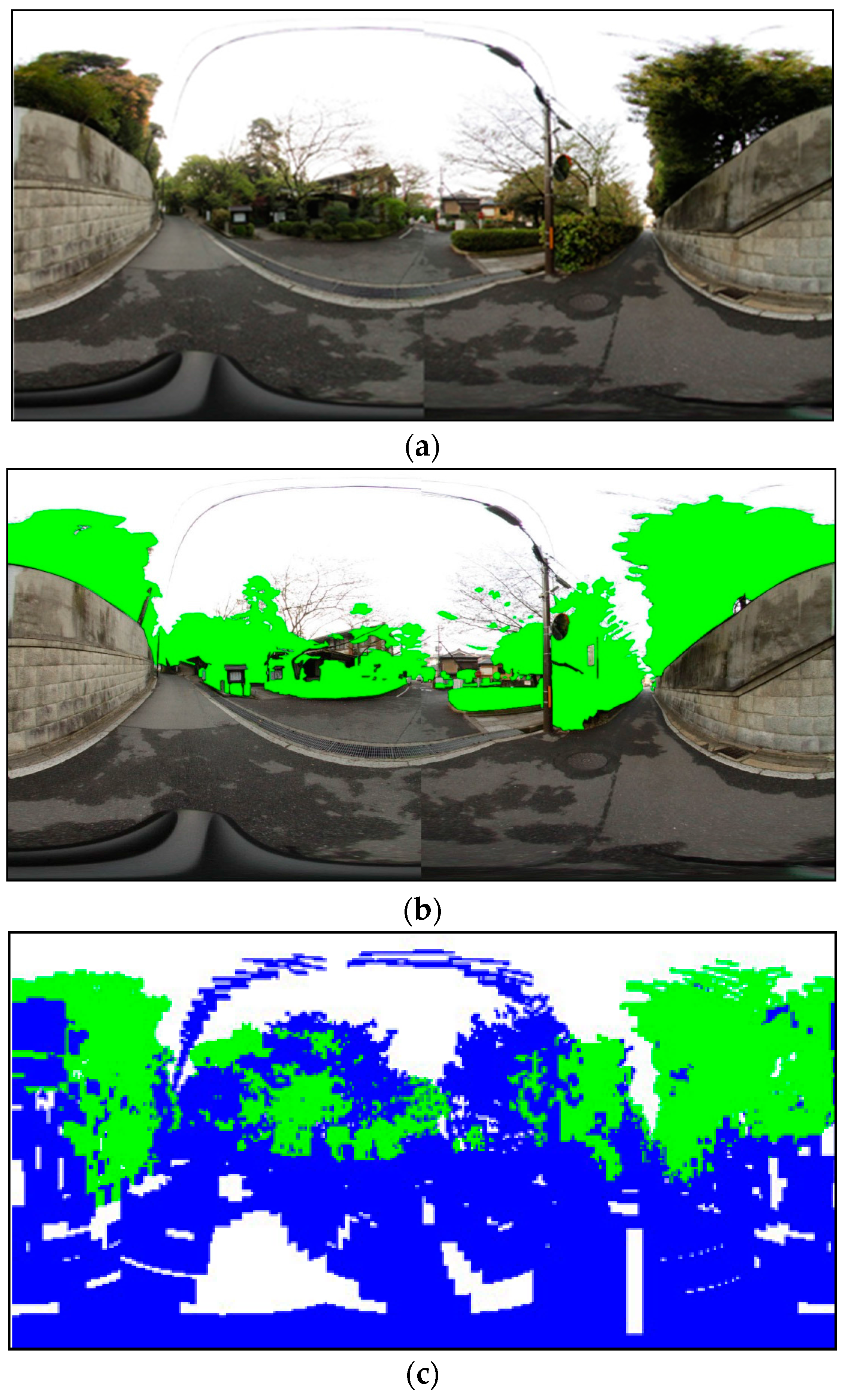
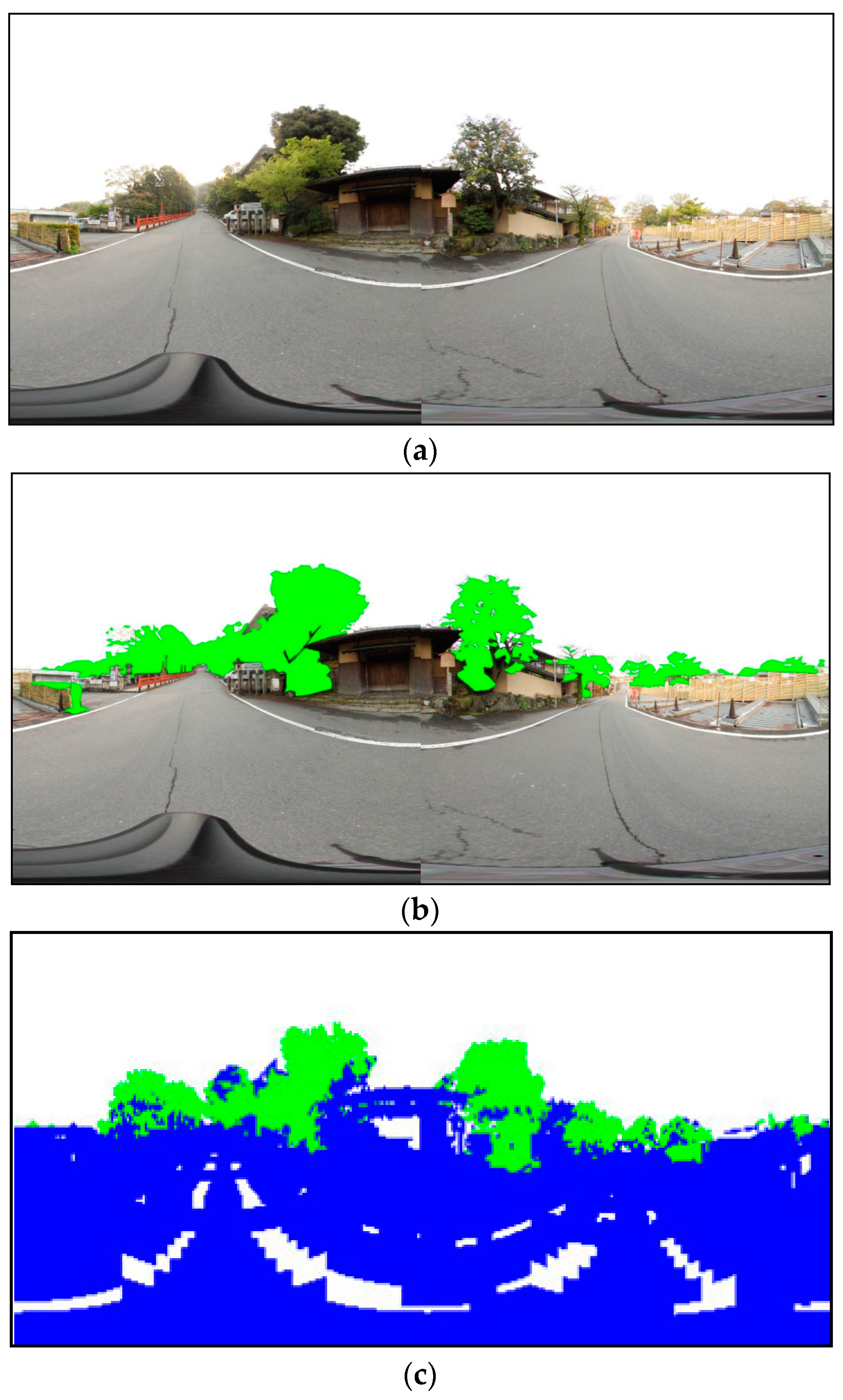
Figure 11 and
Figure 12 show comparisons of the ground truth and the occlusion map obtained by applying the proposed method.
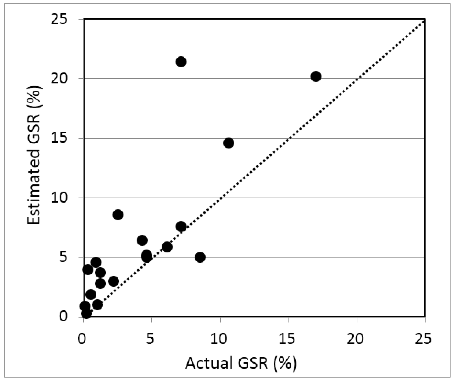
Figure 13 illustrates the comparison of the actual GSR and the estimated GSR. Finally, the RMSE of GSR estimation was found to be 4.1% for 18 points.
6. Discussion
First, we discuss the accuracy of the extracted vegetation and estimated GSR. In vegetation extraction,
Figure 10b shows that the leaves of trees were well extracted, whereas the low box-shaped hedge was not extracted, shown as false negative (FN) in yellow.
Figure 11 and
Figure 12 show the actual view and the occlusion map at P8 and P11, respectively. In the occlusion map, green, blue and white areas represent vegetation, non-vegetation and no-object areas, respectively. The vegetation area drawn in the occlusion map of
Figure 12c corresponds approximately to the area colored in green in the actual view of
Figure 12b, whereas that of
Figure 11c overestimated the vegetation compared to
Figure 11b. As a result, the accuracy of the GSR estimated by the proposed method—an RMSE of 4.1%—was found to be acceptable (
Figure 13) considering that the proposed method is designed to rapidly estimate GSR in wide areas.
The multi-spatial-scale extraction of vegetation implemented in the proposed method functions properly, as shown in
Figure 8 and
Figure 9. Vegetation has various types of 3D shape and surface roughness, and thus the optical spatial scale for extracting vegetation depends on such geometrical features. We take the approach of extracting vegetation using only geometrical information derived from point clouds, not using color information. This approach focuses on extracting geometrical information that reflects vegetation properties that differ from those of non-vegetation. Multi-spatial-scale processing is revealed to be effective for extracting vegetation. However, it falsely extracted as vegetation walls whose surfaces were not flat (
Figure 8b) and branches without leaves. The latter are difficult to extract because they have similar geometrical features to vegetation, that is, they can be regarded as randomly sampled objects.
Next, we focus on the advantage of the proposed method for extracting vegetation and estimating GSR. As explained in
Section 1, some existing approaches use point clouds and images to extract vegetation [
15,
16,
17]. The image requires light source and the brightness of vegetation of the images may depend on the species and measurement season. As a result, the performance of extracting vegetation is not always stable. The proposed approach needs only point clouds and therefore it can avoid such unstable extraction of vegetation. In addition, mobile LiDAR data are found to be effective in estimating small vegetation that airborne LiDAR may have difficulty in extracting. In terms of estimating GSR, the proposed method can estimate it at any point of the study area. Mobile LiDAR can cover much larger areas than stationary LiDAR. The GSR estimated from mobile LiDAR data can represent smaller vegetation than that from airborne LiDAR data.
Then, we address the selection of parameter values. The optimal parameter values for vegetation extraction may be difficult to determine automatically. Therefore, in this research, we repeated manual tuning by applying them to the training data sets. For example, in a previous study we found that the optimal voxel sizes for extracting vegetation from terrestrial LiDAR data were 10 cm and 20 cm [
16]. However, for mobile LiDAR data, we set them to 0.5 m and 1.0 m. We examined several different values, but finally these larger values were found to be optimal.
Figure 8 and
Figure 9 show that different parameter values for voxel size failed to extract vegetation. The optimal parameter values for mobile LiDAR data were found to be different from those for terrestrially fixed LiDAR data. Mobile LiDAR data covers much larger areas than does terrestrial LiDAR data, and accordingly, the range of point density per area of mobile LiDAR data changes much more than that of terrestrial LiDAR data.
Finally, we discuss the factors that contribute to the error in the GSR estimated by the proposed method. First, the estimated GSR tends to be an overestimate. Reconstructed objects become bigger than the actual objects because the voxel-based approach converts point clouds into 0.5 m or 1.0 m voxels. Second, the vegetation around θ = 90° may cause large errors, especially when the point of interest has tall trees and the occlusion map has some vegetation areas around θ = 90°. Voxels around 90° and −90° contribute more to the GSR estimation than does the actual contribution when the projection shown in
Figure 11c and
Figure 12c is used for the occlusion map. This contribution can be reduced using an equisolid angle projection [
21]. Finally, the error in extracting vegetation using point-cloud classification should be resolved. For example, when there is vegetation on a wall or fence, such non-vegetation objects may be falsely extracted as a part of the vegetation. Separating such non-vegetation objects is one of the most difficult challenges in LiDAR data processing. Improving vegetation extraction is a key issue for improving GSR estimation.
7. Conclusions
In this paper, we presented a method for estimating GSR in urban areas using only mobile LiDAR data. The method is composed of vegetation extraction and GSR estimation. Vegetation is extracted by considering the shape of objects on multiple spatial scales. We applied the method to a residential area in Kyoto, Japan. The obtained RMSE of approximately 4.1% was found to be acceptable for rapidly assessing local landscape in a wide area. It was confirmed that mobile LiDAR could extract vegetation along streets and roads, whereas the estimated GSR tends to be an overestimate because of the voxel-based approach. The selection of optimal parameter values depends on the study area, and thus requires manual tuning. However, the proposed method overcame the existing challenge of the automatic vegetation extraction and contributes to assessment of green space even in a complex urban area, that will enrich green landscape. Future tasks are automatic selection of optimal parameter values, and improvement of the accuracy of extracting vegetation points even when there is vegetation on non-vegetation objects.


