Article

Assimilation of Remotely-Sensed Leaf Area Index into a Dynamic Vegetation Model for Gross Primary Productivity Estimation

1
Key Laboratory of Digital Earth Science, Institute of Remote Sensing and Digital Earth, Chinese Academy of Sciences, No. 9 Dengzhuang South Road, Beijing 100094, China
2
College of Resources and Environment, University of Chinese Academy of Sciences, No. 19A Yuquan Road, Beijing 100049, China
3
Key Laboratory of Earth Observation, Sanya 572029, China
4
International Center for Climate and Environment Sciences (ICCES), Institute of Atmospheric Physics, Chinese Academy of Sciences, Beijing 100029, China
5
School of Atmospheric Sciences, Sun Yat-Sen University, Guangzhou 519082, China
6
State Key Laboratory of Earth Surface Process and Resource Ecology, Zhuhai Joint Innovative Center for Climate-Environment-Ecosystem Zhuhai Key Laboratory of Dynamics Urban Climate and Ecology, Beijing Normal University, Beijing 100875, China
7
State Key Laboratory of Remote Sensing Science, School of Geography, Beijing Normal University, Beijing 100875, China
8
Research Faculty of Agriculture, Hokkaido University, Sapporo 0608589, Japan
*
Author to whom correspondence should be addressed.
Remote Sens. 2017, 9(3), 188; https://doi.org/10.3390/rs9030188
Submission received: 19 October 2016 / Revised: 12 February 2017 / Accepted: 20 February 2017 / Published: 23 February 2017

Abstract

:
Quantitative estimation of the magnitude and variability of gross primary productivity (GPP) is required to study the carbon cycle of the terrestrial ecosystem. Using ecosystem models and remotely-sensed data is a practical method for accurately estimating GPP. This study presents a method for assimilating high-quality leaf area index (LAI) products retrieved from satellite data into a process-oriented Lund-Potsdam-Jena dynamic global vegetation model (LPJ-DGVM) to acquire accurate GPP. The assimilation methods, including the Ensemble Kalman Filter (EnKF) and a proper orthogonal decomposition (POD)-based ensemble four-dimensional (4D) variational assimilation method (PODEn4DVar), incorporate information provided by observations into the model to achieve a better agreement between the model-estimated and observed GPP. The LPJ-POD scheme performs better with a correlation coefficient of r = 0.923 and RMSD of 32.676 gC/m2/month compared with the LPJ-EnKF scheme (r = 0.887, RMSD = 38.531 gC/m2/month) and with no data assimilation (r = 0.840, RMSD = 45.410 gC/m2/month). Applying the PODEn4DVar method into LPJ-DGVM for simulating GPP in China shows that the annual amount of GPP in China varied between 5.92 PgC and 6.67 PgC during 2003–2012 with an annual mean of 6.35 PgC/yr. This study demonstrates that integrating remotely-sensed data with dynamic global vegetation models through data assimilation methods has potential in optimizing the simulation and that the LPJ-POD scheme shows better performance in improving GPP estimates, which can provide a favorable way for accurately estimating dynamics of ecosystems.

Graphical Abstract

1. Introduction

Terrestrial gross primary productivity (GPP), the integral of organic carbon fixed through photosynthesis over all of the leaves, is the beginning of the biogeochemical cycle and a primary input for vegetation carbon [1,2]. About half of GPP will be incorporated into new plant tissues (e.g., leaves, roots), and the remainder will be released back into the atmosphere [3,4]. Therefore, quantitative estimates of the magnitude and variability of GPP can enhance further comprehension about the biogeochemical dynamics and the carbon cycle of terrestrial ecosystems.
Numerous ecosystem models, such as the Lund-Potsdam-Jena Dynamic Global Vegetation Model (LPJ-DGVM) [5], have been widely used as a practical method for quantifying temporal and spatial variation of GPP at regional, continental, and global levels. However, considering the spatial-temporal heterogeneity of ecosystem processes, it might be difficult to acquire accurate input parameters of models, thus possibly resulting in low-confidence output results [2,6]. Moreover, the simulation errors caused by the uncertainties of models, both in process mechanisms and related parameters settings, can accumulate gradually and cause results deviating from the true values [7]. Satellite remote sensing data could offer broad spatial-temporal distribution information on vegetation coverage, as well as the state variables of models (e.g., biomass, leaf area index) [8]. Thus, it can be considered as a good option for integration with process-based models to reduce uncertainties in model estimates. Data assimilation (DA) is one technique widely used for combining observation data with process-based models and incorporates real-time data into models constantly to generate a better estimation [7], which can provide a favorable method for accurately analyzing dynamics of ecosystem, expending the use of observations in ecosystem studies. Through assimilation, observed variables are applied to adjust the model state variables; hence, several related variables will be optimized.
The ensemble Kalman Filter (EnKF) algorithm has gained wide attention owing to its simple conceptual formation, optimum performance, and easy implementation [9,10]. Based on the Monte Carlo method, EnKF designs an ensemble of state variables, and the average of the ensemble can be used as the optimal estimation of state variables. Many studies have adopted EnKF for integrating remote sensing data with models in meteorological and hydrological fields [11,12,13,14]. Wang et al. [15] assimilated observed soil moisture into the LPJ-DGVM by using the EnKF method to construct a data assimilation system for optimizing LPJ performance. In the field of land surface vegetation, Ju et al. [16] employed EnKF in optimizing model parameters that significantly improve the simulation of GPP, latent heat (LE), and sensible heat (SH), especially during dry periods. Quaife et al. [17] demonstrated that the assimilation of Moderate Resolution Imaging Spectroradiometer (MODIS) reflectance data into an ecosystem model performed better in improving the estimates of GPP and net ecosystem productivity (NEP).
As a sequential assimilation method, EnKF is naturally designed to deal only with sequential information; therefore, it lacks the temporal smoothness constraint included in the four-dimensional (4D) variational data assimilation (4DVar) method. Research on coupling 4DVar with EnKF has been conducted to fully utilize their respective advantages [18,19,20,21]. Recently, a hybrid method known as the proper orthogonal decomposition (POD)-based ensemble 4D variational data assimilation method (PODEn4DVar), was proposed by Tian et al. [21]. The PODEn4DVar method has the superiority that: (1) the dynamic constraint can use complete simulation equations; (2) it is capable of simultaneously assimilating observations at multiple times; (3) it can reflect the spatial structure of the 4D variables and characteristics of time evolution by using POD-transformed base vectors; and (4) this method does not require an integral adjoint model during the computational process, and it is easy to realize. The PODEn4DVar method can simplify the process of data assimilation and maintain most advantages of the traditional 4DVar method, which has shown considerable satisfactory performance within land data assimilation [22,23], Tan-Tracker joint data assimilation [24], and radar data assimilation [25]. Considering that EnKF and PODEn4DVar each have unique features, each method was applied into LPJ-DGVM separately, and their respective performances were compared in this study.
In this study, we developed a GPP assimilation system for coupling the remotely-sensed leaf area index (LAI) with the LPJ-DGVM dynamic vegetation model, which can be used to optimize the GPP simulation at a given time. The specific objectives of this study were to: (1) apply two assimilation algorithms into the process-based model combined with remotely-sensed LAI data; (2) test and evaluate the ability of different assimilation algorithms within the LPJ-DA system by using six eddy-covariance flux tower sites, and select the optimal model for spatial GPP estimation; and (3) obtain the spatial distribution and calculate the total amount of terrestrial GPP in China during the period of 2003–2012.

2. Study Area and Datasets
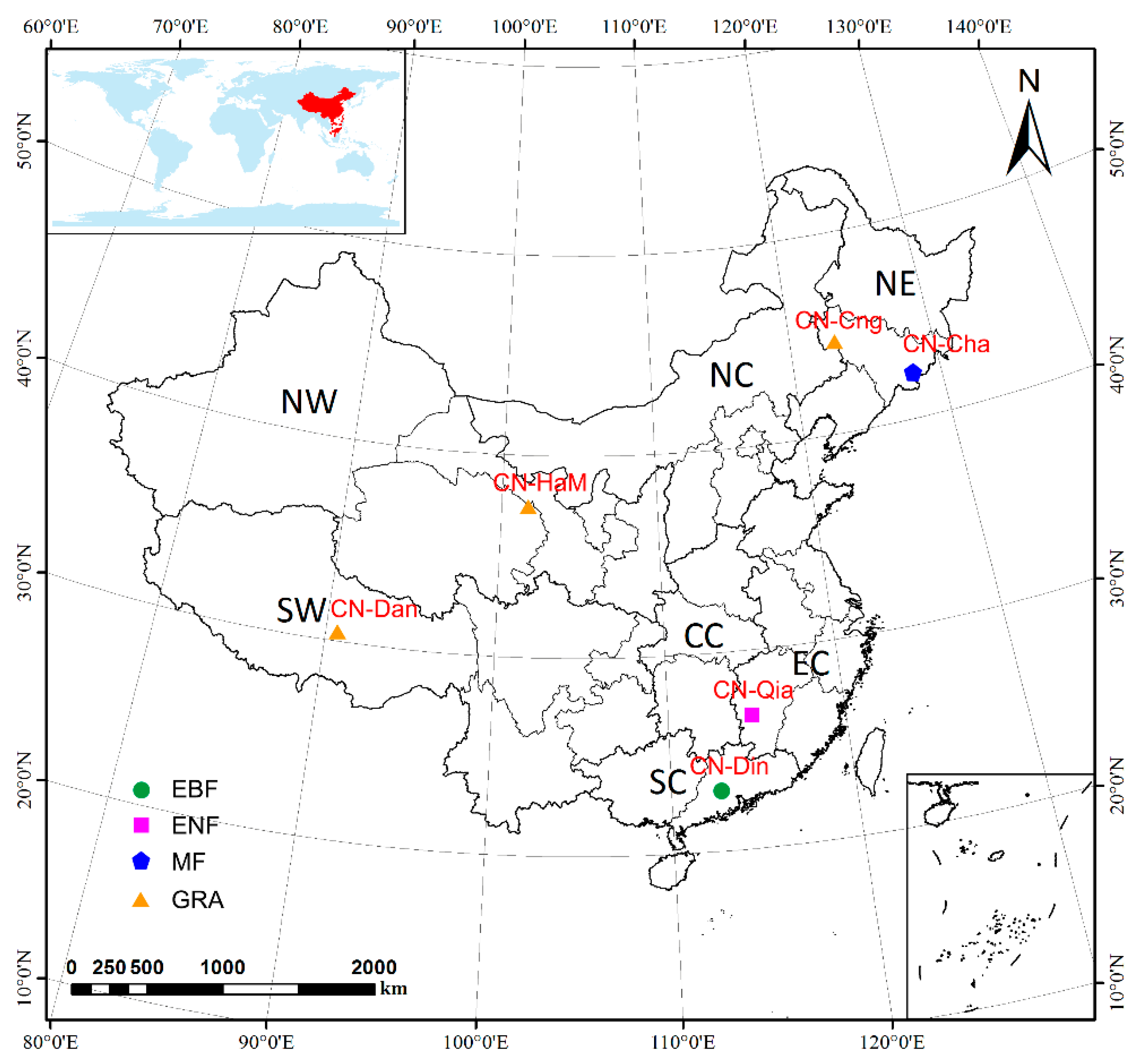
2.1. Study Area

China has a vast territory covering cold, temperate, and tropical zones. Terrains are distributed in a ladder shape, descending from west to east. Mountainous regions and plateaus occupy a large area. With a remarkable monsoon climate, it manifests high-temperature and rainy weathers in summer, and cold and rainless weathers in winter. The contrast of the East Asian summer and winter monsoons, together with the high elevation of the Tibetan Plateau result in a unique terrestrial ecosystem. Over one half of the land area is covered by forests and grasslands. Forests cover about 18.9% of total land area and are located mainly in the south Yangtze River, large and small Xing’an Mountains, and Changbai Mountain to the northeast. Grasslands account for 31.8% and are mainly distributed in most regions of Northwest and North China in addition to the Southwest.

2.2. Flux Tower Measurement

We use the measurements from the FLUXNET2015 Dataset [26] for the verification of the estimations. The six flux tower sites used in this study include four vegetation types: evergreen broadleaf forest (EBF), evergreen needleleaf forest (ENF), mixed forest (MF), and grassland (GRA). Based on previous versions of the FLUXNET Dataset releases (FLUXNET Marconi Dataset 2007 and FLUXNET LaThuile Dataset 2007), the FLUXNET2015 Dataset includes several improvements in data quality control protocols and the data processing pipeline, including close interaction with tower teams to improve data quality, new methods for uncertainty quantification, and use of reanalysis data to fill long gaps of micrometeorological variable records.
Eddy covariance systems give the direct measurement of NEE, and the measured GPP is calculated by subtracting the respiration using a community standard method [27,28]. However, uncertainties remain in the measured GPP values such as underestimation of the total ecosystem respiration (Reco) at night, uncertainties of the gap-filled algorithm, and partitioning and random errors of flux measurements [29,30,31], which may increase the mismatch between measured GPP and simulated GPP. To verify the model results, the six eddy covariance towers including 17 site-years were selected to represent four vegetation types (Figure 1; Table 1). Detailed descriptions of sites information are available at [26].

2.3. Model-Driving Datasets

The input forcing data of LPJ-DGVM was obtained from continuous series of monthly climate data covering the period 1901–2012. This data, consisting of cloud cover, temperature, precipitation, and wet day frequency on a 0.5° × 0.5° global grid [38], was provided by the Climatic Research Unit (CRU), University of East Anglia [39]. Monthly data were linearly interpolated to obtain “quasi-daily” values and were used to simulate processes within LPJ-DGVM at daily time steps. An annual dataset of historical atmospheric CO2 concentrations during 1901–2012 was obtained by combining ice-core measurements and atmospheric observations at the Mauna Loa Observatory in Hawaii [40,41]. Soil texture data was obtained from the Food and Agriculture Organization of the United Nations (FAO) soil dataset [42].

2.4. Remote Sensing Observation

Estimation of LAI from remote sensing data is the feasible method for generating LAI products at regional and, in particular, global scales. The LAI products, such as the MODIS LAI product (MOD15) and the CYCLOPES LAI product, are almost spatially incomplete and temporally discontinuous owing to cloud contamination and are not accurate for certain vegetation types [43,44]. The use of multi-temporal data could be a better strategy for addressing problem of information missing, which is a major feature of Global Land Surface Satellite (GLASS) products. The GLASS product, generated and released by the Center for Global Change Data Processing and Analysis of Beijing Normal University [45], has a temporal resolution of eight-day intervals and spans the period of 1981–2014.
In the GLASS LAI algorithm, general regression neural networks (GRNNs) are trained over the fused LAI from MODIS and CYCLOPES LAI products and pre-processed MODIS/AVHRR surface reflectance of BELMANIP sites. The LAI is retrieved from time-series reflectance data with the trained GRNNs. Direct validation and inter-comparative studies have demonstrated that GLASS LAI has significantly longer temporal ranges, higher spatio-temporal resolution, and improved accuracy compared with other products, such as MODIS LAI and CYCLOPES LAI [44,46].
The GLASS LAI product employed in this study spans the period 2003–2012 at 1 km and eight-day resolution in a sinusoidal projection system. For integrating into the data assimilation modeling framework, we processed the LAI for China and resampled it to 0.5° × 0.5° resolution for consistency with the climatic datasets applied within the LPJ model.

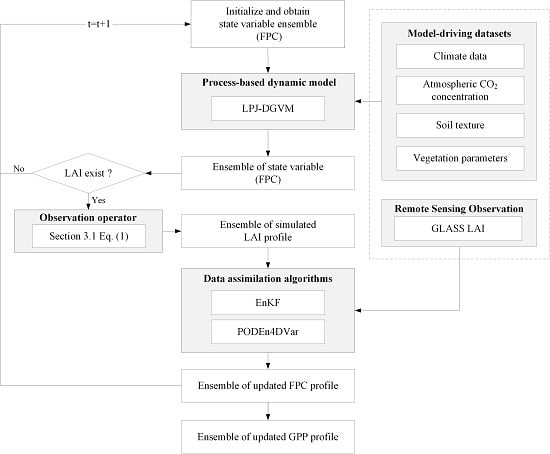
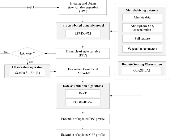
3. Data Assimilation Strategy

A data assimilation system is generally composed of a dynamic model, observation operator, assimilation algorithms, and experiment datasets, including forcing data, model parameters, and observations [7]. In this study, we developed a LPJ-DA modeling framework by using LPJ-DGVM as the model operator to simulate energy and mass exchanges between the surface vegetation and land-atmosphere. To make observations consistent with the state physical and space variables, we linked assimilation algorithms and LPJ-DGVM. We used Equation (1) as an observation operator to convert the simulated foliage projective cover (FPC) state variable into the observed LAI variable when new observations became available. We applied two different assimilation algorithms, EnKF and PODEn4DVar, as discussed in Section 3.2.1 and Section 3.2.2, respectively, to utilize the observation information of GLASS LAI [46], as discussed in Section 2.4. This measure was performed to update the FPC state variable so that the related variables (GPP in this study) can be obtained. A schematic diagram of the LPJ-DA modeling framework is shown in Figure 2.

3.1. Lund-Potsdam-Jena Dynamic Global Vegetation Model

The LPJ-DGVM [5] is a process-based model dealing with the exchange of carbon and water between terrestrial vegetation and land-atmosphere in a modular framework, and inherits many characteristics from the biome family of models [5,47,48,49]. The key features primarily involve feedback through canopy conductance between photosynthesis and water balance, and close coupling among these “fast” processes and other ecosystem processes, including resource competition and production, tissue turnover, growth, carbon cycle in soil and litter, and disturbance regime [5]. For each grid cell, ten plant functional types (PFTs) were defined clearly in terms of FPC, including eight woody and two herbaceous types, with the potential occurrence determined by the bioclimatic limits as a standard for determining whether it can survive and/or regenerate in the simulation. Daily photosynthesis is a function of several abiotic factors including Absorbed Photosynthetically Active Radiation (APAR), day length, biochemical pathway (C3 or C4), atmospheric CO2 concentration, and temperature [5,50]. For each PFT, the GPP is calculated by applying the coupled photosynthesis and water balance. The entire simulation is derived by monthly climate data, soil texture, and atmospheric CO2 concentration in every grid cell.
As an effective method for describing plant community structure, FPC is defined as the vertically-projected percentage cover of photosynthetic foliage of all strata [51], which has an essential relationship with canopy transpiration and radiation interception. Both LAI and FPC can be used to describe the leaf area, and based on the Lambert-Beer Law [52]:
F P C i n d = 1 e ( 0.5 L A I i n d ) ,
where ind represents average individual values. In a grid cell, the entire FPC is calculated by multiplying F P C i n d by the crown area (CA) and population density (P):
F P C t o t a l = C A · P · F P C i n d ,
CA is obtained by applying the stem diameter (D) based on the inversion of Reinecke’s rule [53]:
C A = k a l l o m 1 D k r p ,
where k a l l o m 1 = 100 , k r p 1.6 , and CA is prescribed below a constant C A m a x (15 m2). The daily GPP for each PFT is calculated by combining the FPC from Equation (2), the daily phenological status (have leaves or not), and climate data. The entire calculation of GPP flux is performed for the middle day of each month, and the daily values are derived by interpolation of the mid-month values. In our scheme, the state variable is FPC, and the observed variable is LAI obtained from remote sensing data (GLASS LAI). We selected Equation (1) as the observation operator for integrating the simulation and observation to update the FPC values.

3.2. Assimilation Method

3.2.1. Ensemble Kalman Filter

The EnKF [10,54,55,56], connects the ensemble forecast with the Kalman filter (KF), which makes an implicit assumption that the observations are related to the true state X t (e.g., FPC at time t) by:
Y = H X t + ε ,     ε ~ N ( 0 ,   σ 2 ) ,
where Y is the m-dimensional observation vector, ε is the observation error with average ε ¯ and covariances R = ( ε ε ¯ ) ( ε ε ¯ ) T ¯ , T refers to transposed matrix, and H is the observation operator. Assuming the availability of observation data at time t + 1, the state variable of each corresponding ensemble is updated as:
X i ,   t + 1 a = X i , t + 1 f + P t + 1 f H T ( H P t + 1 f H T + R ) 1 ( Y t + 1 H X i , t + 1 f ) ,
where the superscripts f and a refer to the prior (forecast) and posterior (analysis/updated) estimates, respectively; i represents each individual ensemble number; P t + 1 f represents the error covariance of the state variable.
Since the observation vector Y has a higher dimension (m), EnKF was found to be inefficient when we calculated the inverse matrix shown in Equation (5). To address this issue, a modified inverse calculation was proposed by Liang et al. [57] based on the Sherman-Morrison-Woodbury formula [58]:
( H P t + 1 f H T + R t ) 1 = R t 1 R t 1 Z ( I + Z T R t 1 Z T ) 1 Z T R t 1 ,
Z 1 N 1 [ H ( X 1 , t + 1 f ) H ( X ¯ t + 1 f ) ,     H ( X 2 , t + 1 f ) H ( X ¯ t + 1 f ) ,   ,     H ( X N , t + 1 f ) H ( X ¯ t + 1 f )   ] ,
that is, H P t + 1 f H T Z Z T . Since the total number of disturbing ensembles of state variable N is generally not very high, calculation of the inverse matrix of I + Z T R t 1 Z T is more efficient. As a result, this method can significantly reduce the amount of calculation and enhance the operation efficiency.

3.2.2. POD-Based Ensemble 4D Variational Assimilation Method

On the basis of POD and ensemble forecasting techniques, Tian et al. [21] proposed a hybrid method: the POD-based ensemble 4-D variational assimilation method (PODEn4DVar). This method uses linear combinations of the transformed model perturbations (MPs) and observation perturbations (OPs) to express the optimal MP and its OP, respectively. Moreover, this method can assimilate multiple-time observation data and update its background error covariance by integrating the advantages of variational methods and evolving forecast ensembles. By minimizing the incremental format of the cost function in the 4DVar algorithm, an optimal increment of initial condition can be achieved at the initial time by:
J ( x ) = 1 2 ( x ) T P b 1 ( x ) + 1 2 [ y ( x ) y o b s ] T R 1 [ y ( x ) y o b s ] ,
where x = x x b , y = y ( x ) = y ( x ) y ( x b ) , y o b s = y o b s y ( x b ) , and y = H [ M t 0 t k ( x ) ] . Here, the b represents the background field, index k stands for the observation time, P b is the background error covariance, and obs denotes observation.
Applying the POD transformation, the optimal solution can be expressed as:
x a = P x β   y a = P y β ,
The background error covariance P b can be calculated from:
P b = P x P x T N 1 ,
where N is the size of the ensemble. By substituting Equations (9) and (10) into the Equation (8), we obtain another cost function with control variables β instead of x :
J ( β ) = 1 2 ( N 1 ) β T P x T ( P x T ) 1 ( P x ) 1 P x β + 1 2 ( P y β y o b s ) T R 1 ( P y β y o b s ) ,
marking P a = [ ( N 1 ) I + P y T R 1 P y ] 1 , the incremental analysis x a is expressed by:
x a = P x P a P y T R 1 y o b s ,
therefore, the final analysis x a can be calculated as:
x a = x b + x a = x b + P x P a P y T R 1 y o b s ,
To ameliorate the spurious long-range correlations between observation locations and model variables resulting from the ensemble-based method, a localization technique is applied to the calculations process [59]. The final analysis is rewritten as:
x a = x b + C 0 ( d h d h , 0 ) · C 0 ( d v d v , 0 ) · x a ,
where d h and d v are the horizontal and vertical distances between the spatial positions of state and observed variables, respectively; and d h , 0 and d v , 0 are the horizontal and vertical covariance localization Schur radii, respectively. The filtering function C 0 is expressed as:
C 0 ( r ) = { 1 4 r 5 + 1 2 r 4 + 5 8 r 3 5 3 r 2 + 1 , 0 r 1 1 12 r 5 1 2 r 4 + 5 8 r 3 + 5 3 r 2 5 r + 4 2 3 r 1 , 1 < r 2 0 , 2 < r ,
where r is the radius of the filter.

3.3. Model Performance
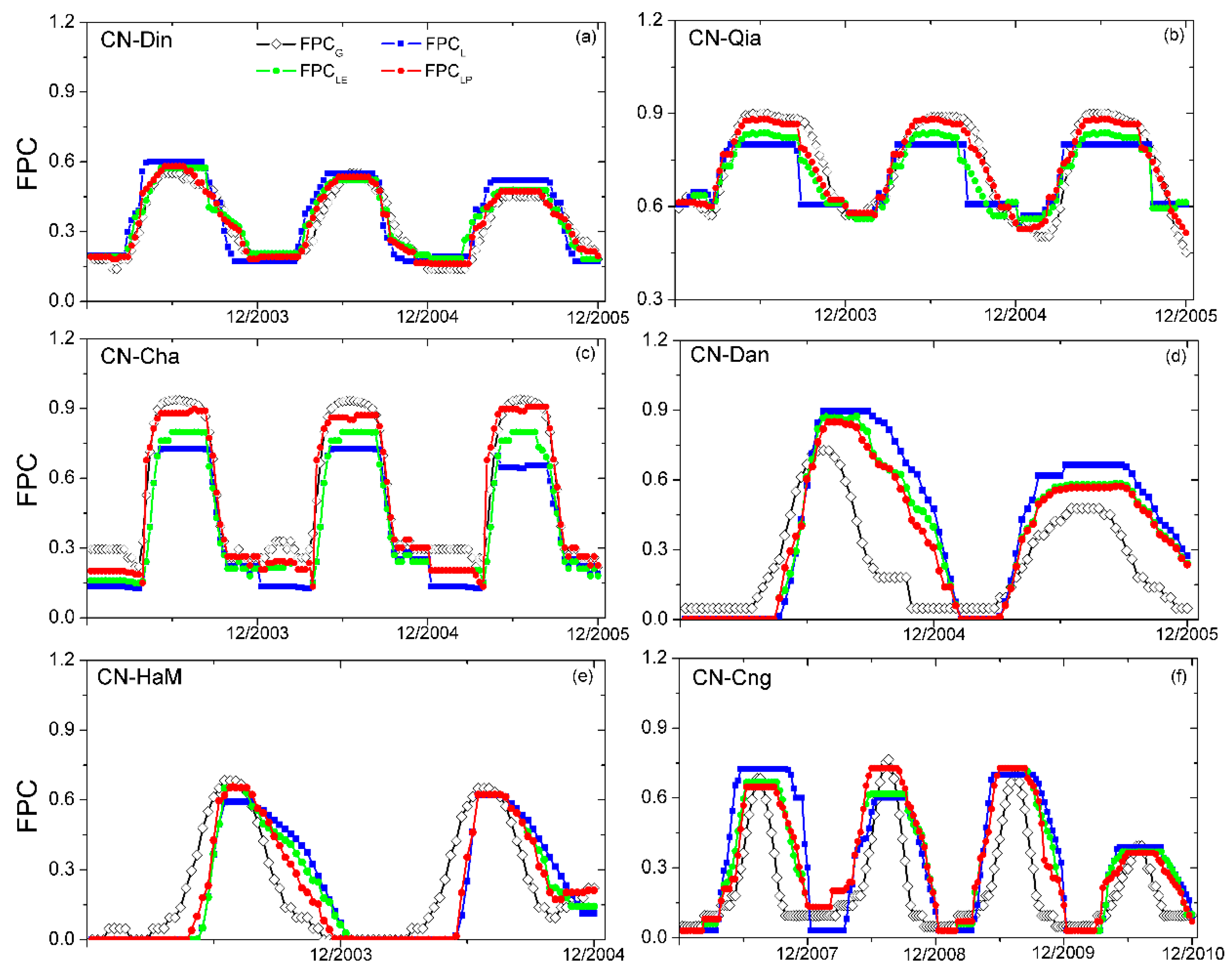
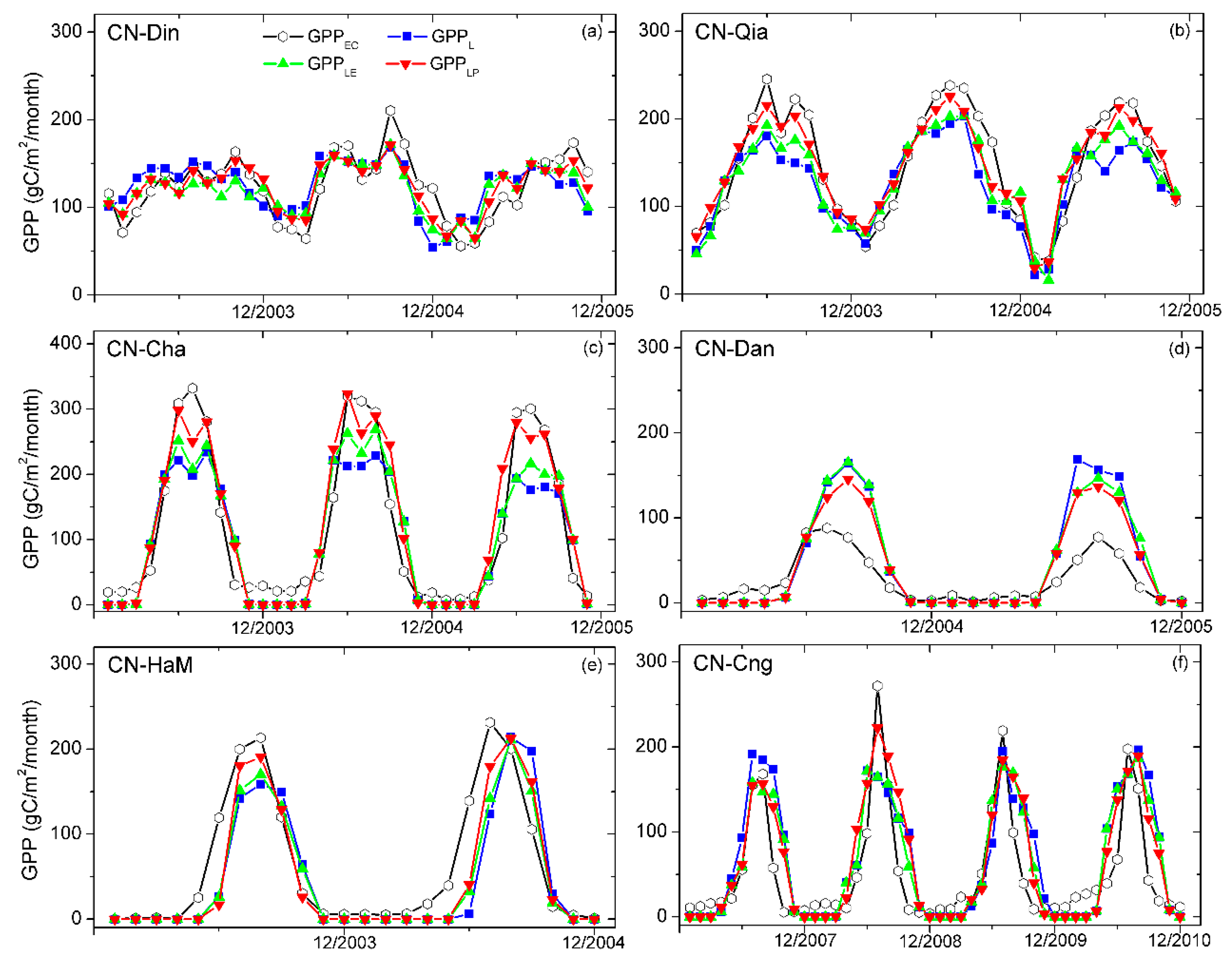
Pearson’s correlation coefficient (r), standard deviation (SD), root-mean-square difference (RMSD), and centered RMSD (CRMSD) are used to quantify model accuracy and agreement using six flux tower sites. In this study we consider the flux-derived GPP as the “ground truth”, though we acknowledge that the flux tower measurements may contain instabilities in observation caused by the contamination of atmospheric and cloud, and instrument errors.
r = i = 1 n [ ( G P P m o d e l G P P m o d e l ¯ ) · ( G P P E C G P P E C ¯ ) ] ( n · S D m o d e l · S D E C ) ,
S D = i = 1 n ( G P P G P P ¯ ) 2 n   ,
R M S D = i = 1 n ( G P P m o d e l G P P E C ) 2 n   ,
C R M S D = i = 1 n [ ( G P P m o d e l G P P m o d e l ¯ ) ( G P P E C G P P E C ¯ ) ] 2 n   ,
Here, G P P m o d e l and G P P E C represent the estimated and observed GPP values, respectively; G P P m o d e l ¯ and G P P E C ¯ are the mean values of estimated and observed GPP values, respectively; and n is the number of observations.
The Taylor diagram [60] provides a concise and graphical statistical summary of r, CRMSD, and SD of the observed and estimated patterns on 2D plots. In this paper, we normalized SD and CRMSD (NSD and NCRMSD, respectively), to display and compare the performances of all flux towers in one diagram [61].
N S D = S D m o d e l / S D E C ,
N C R M S D = C R M S D / S D E C ,
Here, r, NSD, and NCRMSD are not independent, but are related by the following formula:
N C R M S D = N S D 2 + 1 2 × S D × r ,
In the Taylor diagram, NSD is expressed as a radial distance from the origin and the correlation with tower-based data as an angle in the polar plot. The distance to the observation point is proportional to NCRMSD between the estimated and observed values. The simulated points having good agreement with observations lie nearest to the point identified as “observed” on the x-axis. This diagram is especially practical and visual in evaluating multiple aspects of various models.
In addition to the aforementioned indices, the relative RMSD (RMSDr) is calculated as a proportion of the mean estimated value [62] as:
R M S D r = ( R M S D / G P P m o d e l ¯ ) × 100 % ,

4. Results

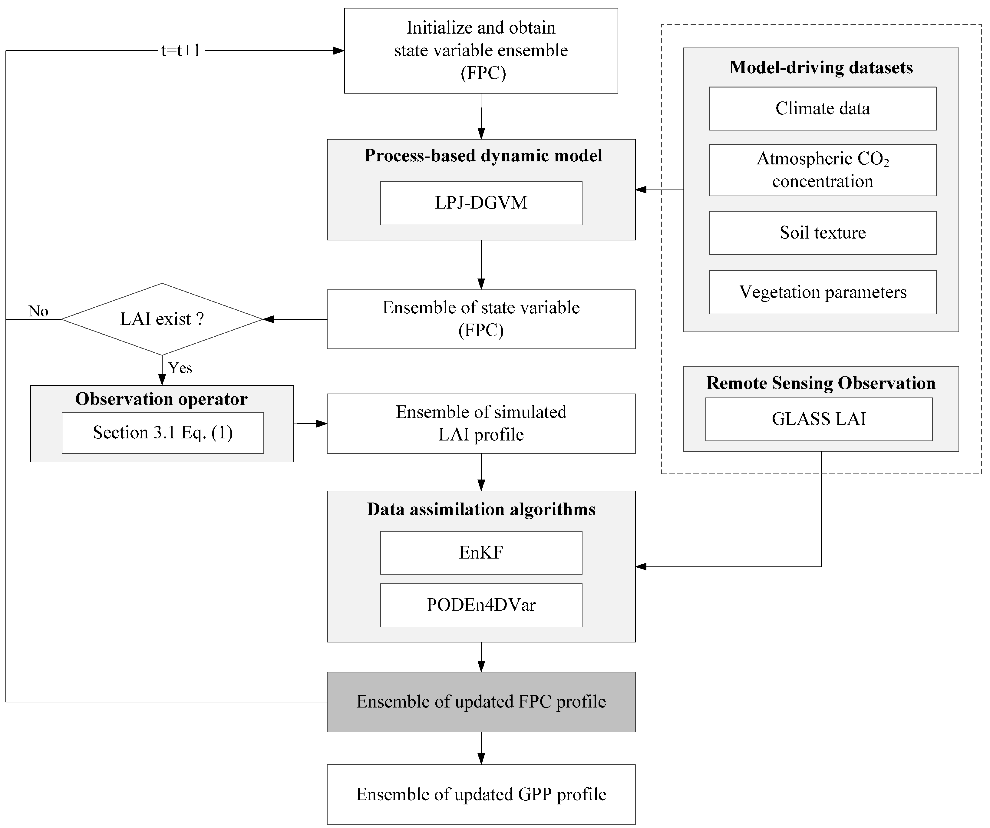
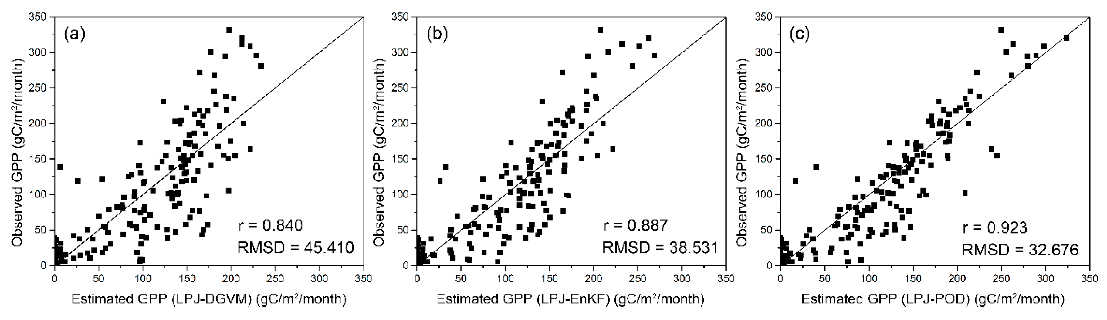
4.1. Accuracy Assessment of Simulated GPP

In this experiment, we assimilated ten years of GLASS LAI products into the LPJ-DGVM to update FPC beginning in 2003. The temporal trends of estimated and assimilated results of FPC at six sites are given in Figure 3, depicted as: FPCL (FPC simulated from LPJ-DGVM), FPCLE (FPC simulated from the assimilated LPJ-DGVM using the EnKF), and FPCLP (FPC simulated from the assimilated LPJ-DGVM using the PODEn4DVar). FPCG represented GLASS FPC (calculated from GLASS LAI products using Equation (1)).
Notably, the estimation of FPC with assimilation has great improvement in most sites. We can see that the simulated FPC with assimilation at Figure 3a obviously corrected the modelling tracks of the LPJ-DGVM, improving the original model which overestimates in peak value and slightly underestimates in winter. Figure 3b,c showed higher estimated FPC compared with FPCG, especially at the peak of the growing season, but the assimilated FPC followed GLASS FPC closer than the simulated FPC and can capture the variation of FPC exactly at these two sites. As shown in Figure 3d–f, the simulated results without assimilation clearly overestimated after the peak of the growing season, while results with assimilation significant decreased margin between estimated and remote-sensed values. It is noticeable that FPCLP performed much better than FPCL and FPCLE, and the estimated results are quite consistent with the FPCG, especially for the growing season of forests (Figure 3a–c).
The seasonal variations of estimated and observed GPP at six sites in China during 2003–2010 are given in Figure 4a–f. GPPEC, GPPL, GPPLE, and GPPLP were the abbreviations of GPP from eddy-covariance observations and Lund-Potsdam-Jena (LPJ), LPJ-Ensemble Kalman Filter (LPJ-EnKF), and LPJ-proper orthogonal decomposition (LPJ-POD) schemes. The results showed that schemes with assimilation can exactly retrieve GPPEC by integrating remote-sensed information. At the CN-Din and CN-Qia sites (Figure 4a,b), good agreement was shown for both GPPLE and GPPLP with GPPEC. Both tracked the seasonal dynamics of GPPEC well but underestimated the value when it captured the peak of the growing season in 2004. At the CN-Qia site, there was an apparently underestimation for GPPL, but was improved greatly with the PODEn4DVar method. At the CN-Cha site (Figure 4c), GPPLP was much closer to the observed values at the peak of the growing season. However, data assimilation did not show obvious advantages at the CN-Dan site (Figure 4d), with three schemes having higher GPP values than observations. This was consistent with results shown in Figure 3d, with all schemes displaying higher FPC than FPCG. The estimated GPP showed later initiation, but captured the cessation of the growing season for the CN-HaM site (Figure 4e). GPPL overestimated GPP to a large extent after August for the CN-Cng site (Figure 4f), indicating that assimilation can accurately retrieve GPP by adding remotely sensed LAI. Before and after the peak of the growing season at the CN-Cng site, all of the estimated GPP values were significantly overestimated. The GPPLE values were very close to GPPL at several site-years (e.g., CN-Dan 2004, CN-Cng 2008), which indicated that the EnKF method did not make significant improvements. However, the GPPLP for these site-years showed greater consistency with GPPEC and were significantly closer to the observed GPP.
Figure 5 quantifies the similarity between simulated and observed GPP in terms of their correlation, normalized centered RMSD, and relative amplitude of variations represented by normalized SDs by withholding 17 site-years (No. 1 to No. 17, Figure 5a) and four PFTs (A to D, Figure 5b) including EBF, ENF, MF, and GRA. Only the site-years or PFTs with p-values <0.05 were considered. An ideal model manifested as NSD of 1.0 and r of 1.0. The points between the two black dashed lines in the figure represented the site-year or PFTs with 0.7 N S D 1.3. The excluded site-years were CN-Din 2003 (No. 1, GPPL, p-value > 0.05) and CN-Dan 2005 (No. 11, NSD > 2.0). Points lying on the red solid line indicated estimated GPP having variations similar to those of the observations. The position of each point on the two plots quantified the agreement between simulated GPP and observations.
Sites with large or small NSD showed inconsistency between simulated and observed GPP. Therefore, we considered that the points between two dashed lines (with 0.7 N S D 1.3) had similar variability with the observations, and we further grouped them into three levels based on the correlation values: I (0.7 < r ≤ 0.8), II (0.8 < r ≤ 0.9), III (0.9 < r ≤ 1.0). All of these points showed better performance than other points (with NSD < 0.7 or NSD > 1.3 and r ≤ 0.7), and the higher correlation coefficient presented better consistency with the observations.
As shown in Figure 5 the GPP values with data assimilation behaved better in terms of correlation, especially for III (0.9 < r ≤ 1.0) with correlations of 7/17 (seven points meet the requirement in 17 site-years) for both of two assimilation methods. For all site-year, the total proportion within the scope of 0.7 N S D 1.3 and r > 0.7 increased by 87.5% from both GPPL (8/17) to GPPLE (15/17), and GPPLP (15/17). GPPLP performed better with higher proportion (8/17) than GPPL (4/17) and GPPLE (4/17) for II (0.8 < r ≤ 0.9). Moreover, the correlation of certain site-years (e.g., CN-Din) was substantially improved by more than 0.2 when using the PODEn4DVar method, and exhibited stronger correlations (generally r > 0.85) with the site observations than the values from LPJ and LPJ-EnKF schemes (Table 2).
For four PFTs, a similar situation is shown in Figure 5b. The results with data assimilation generally agreed well with observations, with higher correlation and NSD closer to 1. Point A (PFT: EBF), apparently, had been greatly improved by using assimilation method (improving r by 0.141 and 0.249 for GPPLE and GPPLP, respectively, and N S D getting closer to 1) (Figure 5b, Table 3). Point D (PFT: GRA, GPPL) did not exist between the two dashed lines owing to its higher NSD, which increased the distance from the red solid line, but it had been improved by PODEn4DVar method with a higher correlation and lower RMSD. Overall, GPPLP had a higher proportion and higher correlation with 0.7 N S D 1.3; all of the PFTs were present between the dashed lines. This showed obvious improvement in all statistical indices over values without assimilation, especially for evergreen needleleaf forest and mixed forest, with r > 0.94 (Table 3). In general, the PODEn4DVar method performed slighter better with r = 0.923 and RMSD = 32.676 gC/m2/month than LPJ-DGVM (r = 0.840, RMSD = 45.410 gC/m2/month) and LPJ-EnKF (r = 0.887, RMSD = 38.531 gC/m2/month) schemes (Figure 6). It can be concluded that PODEn4DVar had the best advantage for improving model estimations when integrated in dynamic vegetation models.

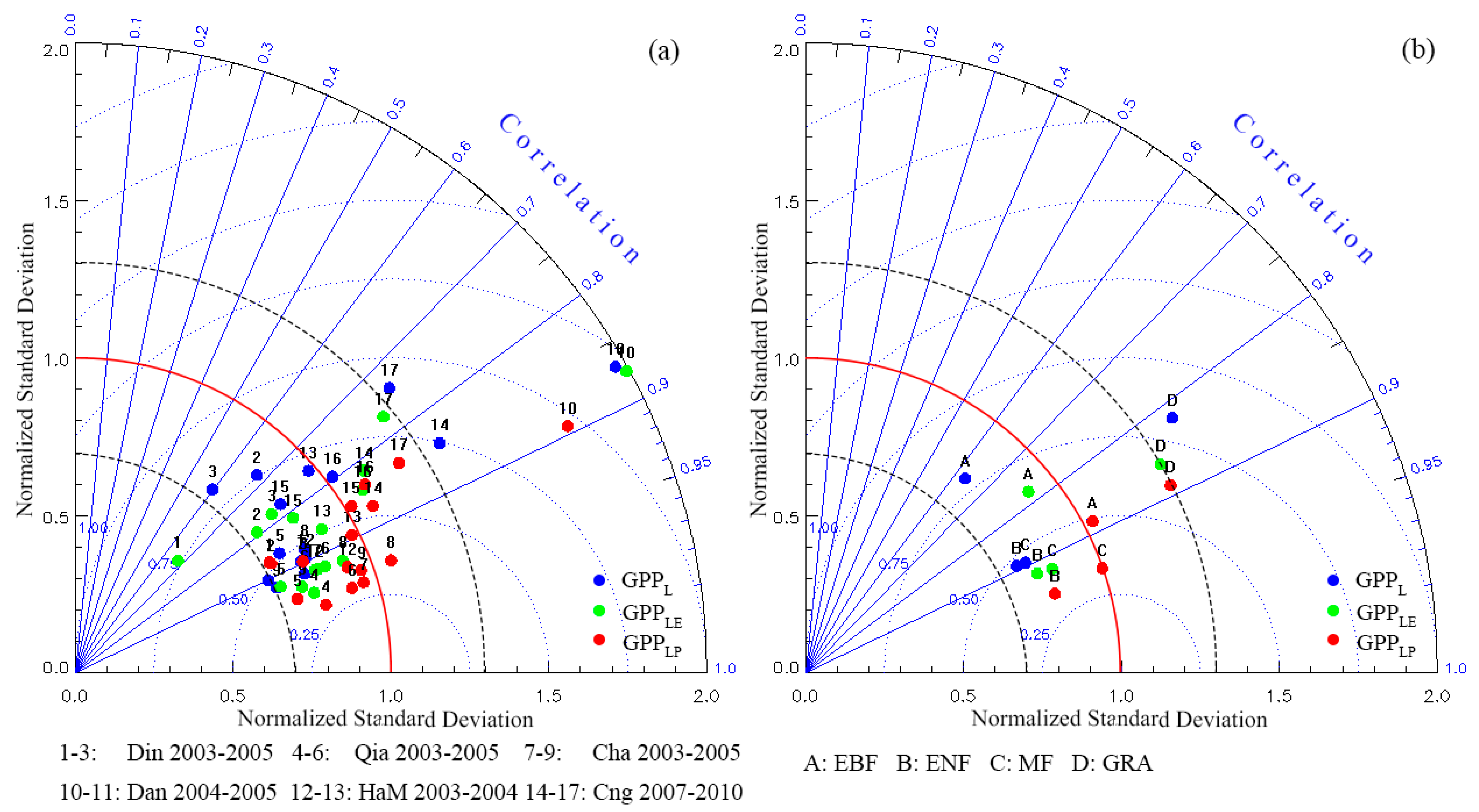
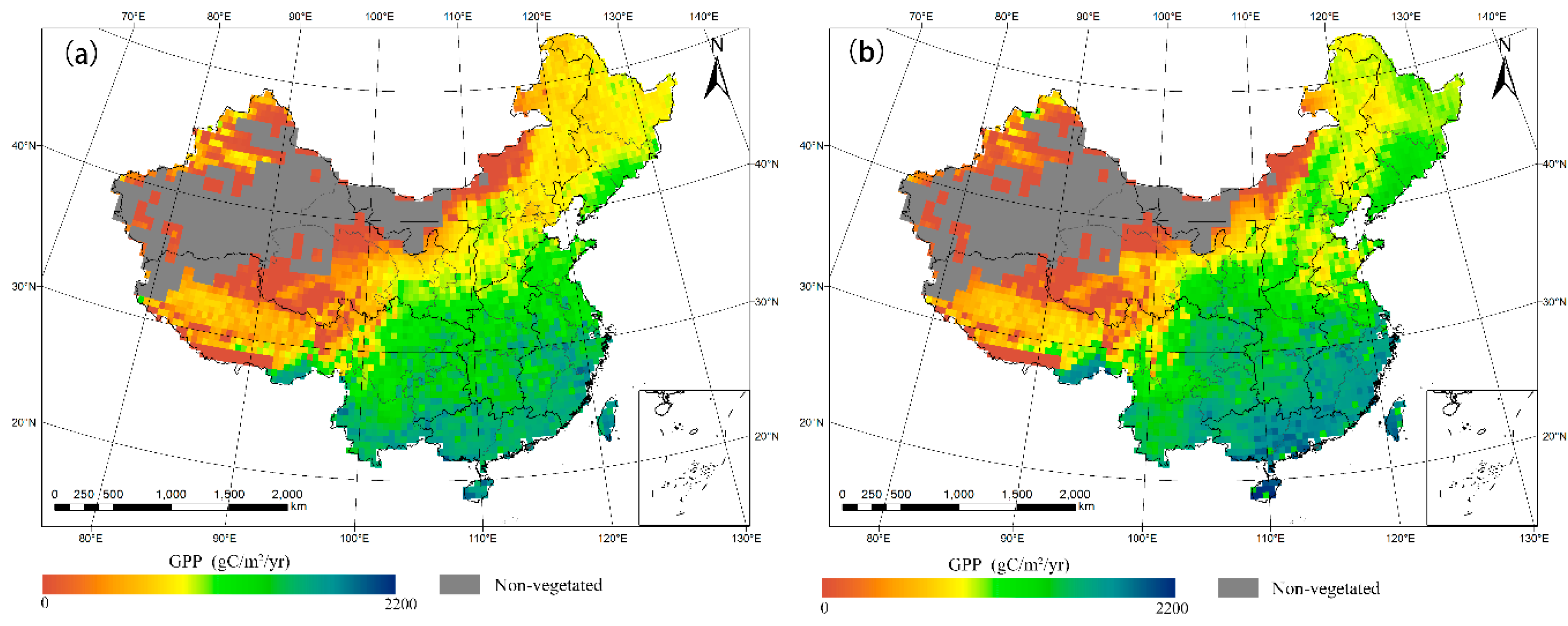
4.2. China’s Terrestrial GPP

The spatial distributions of terrestrial GPP in China over the period 2003–2012 were generated from our LPJ-POD data assimilation system, and their averages are given in Figure 7a (pixel size 0.5° × 0.5°). Similar distribution trends were found from 2003 to 2012, with a decreasing gradient from the southeast toward the northwest regions, as suggested in previous studies [63,64]. The highest GPP estimate (>2000 gC/m2/yr) appeared in the Yunnan province, Southeastern Tibet, south of East and South China, mainly with a distribution of evergreen and mixed forests. Warm temperature, plentiful precipitation, and sufficient radiation in these regions provided an advantageous environment for vegetation growth. The lowest GPP (<700 gC/m2/yr) was concentrated in large portions of Tibet and Northwest China and in central regions of Inner Mongolia province, which is partially covered by ice, bare soil, and rock in a relatively cold climate with scarce precipitation [65].
The SD was applied to indicate inter-annual variability of the GPP during the period 2003–2012 (Figure 7b). Relatively high SD appeared in most of North China, the northeast area of Northwest China, north of East China, and south of Southwest China, indicating greater volatility in these areas.
The LPJ-POD scheme determined that the average annual GPP in China from 2003 to 2012 was about 6.35 PgC/yr, with estimates ranging from 5.92 PgC/yr in 2003 (Figure 8a) to 6.67 PgC/yr in 2012 (Figure 8b). The GPP in 2003, 2006, and 2007 showed relatively low values, at 5.92 PgC/yr, 6.15 PgC/yr, and 6.18 PgC/yr, respectively. Drought conditions occurred frequently and became a major limitation to plant growth and development, especially the drought stress that occurred during the summer of the three years [66,67,68]. In spring 2003, a rainfall shortage caused droughts on a large scale in the northeast. Sustained high temperature and diminished rainfall caused a severe drought in South China during the summer and autumn periods of 2003, and a wide range of regional drought severely affected the photosynthetic activities of plants, thus affecting ecosystem productivity [66]. Compared with the drought years of China, 2012 was a year with less meteorological drought, although the northern regions of Central China and East China experienced moderate or severe droughts during May and June [69].

5. Discussion

Ecosystem models can provide a description of the complex vegetation dynamics of the ecosystem, but only by a simplified presentation of the actual situation. There are many approximations, assumptions, and uncertainties that will increase the uncertainties in the terrestrial GPP estimates. Data assimilation methods have been used to improve the performance of the processed model and reduce errors in model simulation [15,16,17,70,71,72]. Most studies regarding assimilating observation data into the ecosystem models mainly focused on the evaluation of the EnKF approach for ecological forecasting. Though EnKF can give an optimum estimate of GPP at the next moment of model simulations, it does not provide an analytical solution of overall balance. Other assimilation algorithms, like 4DVar, may be adopted so that the entire model trajectory will be affected by the observations and an analytical solution of overall balance will be obtained [18]. To make productivity estimates more precise, a combination of different assimilation approaches should be considered. The PODEn4DVar adopted by this paper complements the advantages and disadvantages of EnKF and 4DVar well, which can simultaneously assimilate multi-time and multi-source observations, providing the overall balance analysis solution and the error estimates with flow-dependence [21]. The results of statistical analysis indicate that the simulated GPP from the LPJ-POD scheme has been improved significantly compared with the LPJ and LPJ-EnKF schemes. This study is generally encouraging for the further application of the PODEn4DVar method integrating with dynamic vegetation models, to reduce uncertainty of terrestrial carbon flux estimates at different scales.
The performance of data assimilation schemes may also be affected by the quality of observation data. Currently, most studies have investigated the capability of assimilating MODIS LAI product into the process-based models [72,73,74]. However, the MODIS LAI product lacks adequate stable profiles, especially for the growing seasons [44]. Zhao et al. [72] have adopted a Savizky-Golay filter to resolve the discontinuous performance of MODIS LAI arising from snow cover, cloud, and sensor errors during the crop growth stages, but the filter has brought new errors which will decrease the higher LAI and create abnormal lower values when involving the universal low LAI values. Xiao et al. [44] proposed a method for retrieving a long time series GLASS LAI product from multi-temporal data. The retrieval algorithm used annual observations to generate the LAI annual profile, which can remove abrupt spikes and dips effectively and produce temporally continuous LAI product. Therefore, we assimilated high-quality GLASS LAI sequentially into the LPJ model to renew the FPC that is related to photosynthesis. The better performance for GLASS LAI than the MODIS LAI were validated through the quantitative comparison at site of different biomes [44].
Though our LPJ-POD scheme successfully improved the modeling accuracy, and explicitly described the spatial distributions of GPP in China during the period 2003–2012, there were still some uncertainties. For six selected sites, overestimated and underestimated GPP remained at a few site-years. This discrepancy also raised the inaccuracy of the temporal and spatial features of the simulated GPP at the regional scale. The uncertainty was partly owing to the model structure. First, one limitation is that many critical parameters provided as default values in LPJ will induce uncertainty in simulating ecosystem carbon fluxes [75,76,77]. For each grid cell, the LPJ-DGVM simulated potential vegetation distribution according to several bioclimatic limits [5], which would bring deviations if simulated vegetation compositions are different from actual composition of the PFTs in the cell. For example, the potential vegetation types simulated by the LPJ-DGVM of the CN-Dan (FPT: GRA) are C3 perennial grass and boreal broadleaved summergreen tree. The simulated GPP of CN-Dan showed sizable higher values due to a large percentage of C3 perennial grass was simulated as summergreen tree. Moreover, it is indicated that default leaf longevity may cause significant differences of terrestrial carbon flux estimation, and other parameters, such as turnover times of the leaf, sapwood, and fine root, also need to be revised to reduce uncertainties [75]. Second, previous research has found that plant photosynthesis and runoff are particularly sensitive to air temperature, which will be affected by the interpolation of monthly temperature to “quasi-daily” values [78,79]. Third, empirical or simplified algorithms were adopted in the LPJ model to simulate the ecosystem carbon cycle, which also induced uncertainties in model outputs [5]. Considering the poor performances of the LPJ model in calculating the water cycle process, it is necessary to assimilate soil moisture into the model to constrain some model parameters such as sensible and latent heat fluxes [15] and, hence, decrease the mismatch between simulation results and observations.
Our GPP estimates also have other sources of uncertainty. Though GLASS LAI is widely used for modeling research, it cannot be the same as the ground-measured LAI. Moreover, the LPJ model is usually influenced by uncertainty of several crucial parameters, such as soil texture and atmospheric driving data, including temperature, precipitation, and cloud cover [7]. These errors could propagate to the final GPP values and eventually cause deviation of the model estimates from the observed data. To optimize the model outputs, incorporating the remote sensing model into the LPJ-POD scheme by calibrating sensitive parameters of the LPJ model [71,80] will be also considered in further work.
In this study, GPP simulated by the optimal scheme (LPJ-POD) in China was comparable to previous studies. At the national scale, the GPP estimates exhibited strong discrepancies from various ecosystem models (Table 4; [63,64,81,82,83,84]). A higher terrestrial annual productivity estimate of 12.26 PgC in China was obtained from a remote sensing model [83], which is almost the equivalent of twice the GPP estimates of this study and Li et al. [63]. Liu et al. [82] constructed a daily driving Terrestrial Ecosystem Production process model (TEPC) and gave a relative higher vegetation production of 7.356 PgC/yr in China based on the Boreal Ecosystem Productivity Simulator (BEPS) and the bio-geochemical model (Biome-BGC). Based on the analysis of published terrestrial productivity in China, lower productivity focused mostly on Carnegie-Ames-Stanford Approach (CASA), BIOME-BGC and BEPS, and the results revealed that the averaged GPP in China was 5.656 Pg/yr according to the 16 studies on terrestrial productivity of China [85], which is 10% lower than GPP estimates in our study. Different model performance of GPP estimates in China owing to different definition of vegetation dynamic, parameter settings, and simulation algorithms. Our developed LPJ-POD system provides an effective way to constrain parameter values and makes model outputs closer to the observation data, which can be a comparative method when estimating China’s annual GPP.

6. Conclusions

In this study, we developed a GPP assimilation system based on EnKF and PODEn4DVar algorithms. Eddy covariance flux datasets of six sites provided by FLUXNET2015 were adopted for validating the performances of GPP values estimated by two assimilation methods (GPPLE, GPPLP) and no assimilation method (GPPL). The optimal method was applied to assess the spatial distribution of GPP values in China during the period 2003–2012. Results showed that the EnKF and PODEn4DVar methods were reasonable for application to the LPJ model, showing better correlation and smaller RMSD. The LPJ-POD scheme performed better, with an r of 0.923 and RMSD of 32.676 gC/m2/month compared with the LPJ-EnKF scheme values of r = 0.887, 38.531 gC/m2/month and the LPJ scheme with r = 0.840, 45.410 gC/m2/month. According to the results of the optimal method, the LPJ-POD scheme, the annual GPP values in China from 2003 to 2012 varied between 5.92 PgC/yr (2003) and 6.67 PgC/yr (2012) with a mean of 6.35 PgC/yr.
This study demonstrated that integrating remotely-sensed data with dynamic global vegetation models through data assimilation methods has potential for simulation optimization and that the LPJ-POD scheme showed better performance in improving GPP estimations. However, our developed LPJ-POD scheme still has uncertainties both in the magnitude and spatial distribution of the GPP at the national scale. To improve process-based models and obtain better simulated results, integrating with a remote sensing model, such as CASA, to calibrate ecophysiological parameters of the LPJ model is a further step for future study.

Acknowledgments

This study was supported by the National Natural Science Foundation of China (NSFC) (Grant No. 41271372), the Innovation Team Program of Hainan Natural Science Foundation (Grant No. 2016CXTD015), and the Major Programs of High–Resolution Earth Observation System (Grant No. 32-Y2-0A17-9001-15/17). The work used eddy covariance data acquired and shared by the FLUXNET community, including ChinaFlux and USCCC networks. The authors would also like to thank to the Center for Global Change Data Processing and Analysis of Beijing Normal University for providing the GLASS LAI products. The authors appreciate the constructive comments on the manuscript offered by anonymous reviewers and editors.

Author Contributions

Rui Ma conducted the experiments, processed the data, analyzed the results, and wrote the majority of the manuscript. Li Zhang designed the main concept of the study, supervised and provided instructions for the research work, and contributed to the manuscript structure and discussions. Xiangjun Tian developed the PODEn4DVar method and helped with discussions and modification of the manuscript. Jiancai Zhang contributed to the experiments and helped with discussions. Wenping Yuan, Yi Zheng and Tomomichi Kato helped with discussions and revisions. Xiang Zhao provided and processed the GLASS LAI products for the experiments.

Conflicts of Interest

The authors declare no conflict of interest.

References

  1. Ichii, K.; Kondo, M.; Okabe, Y.; Ueyama, M.; Kobayashi, H.; Lee, S.; Saigusa, N.; Zhu, Z.C.; Myneni, R.B. Recent Changes in Terrestrial Gross Primary Productivity in Asia from 1982 to 2011. Remote Sens. 2013, 5, 6043–6062. [Google Scholar] [CrossRef]
  2. Yuan, W.P.; Liu, S.G.; Yu, G.R.; Bonnefond, J.; Chen, J.Q.; Davis, K.; Desai, A.R.; Goldstein, A.H.; Gianelle, D.; Rossi, F.; et al. Global estimates of evapotranspiration and gross primary production based on MODIS and global meteorology data. Remote Sens. Environ. 2010, 114, 1416–1431. [Google Scholar] [CrossRef]
  3. Gebremichael, M.; Barros, A.P. Evaluation of MODIS Gross Primary Productivity (GPP) in tropical monsoon regions. Remote Sens. Environ. 2006, 100, 150–166. [Google Scholar] [CrossRef]
  4. Kotchenova, S.Y.; Song, X.D.; Shabanov, N.V.; Potter, C.S.; Knyazikhin, Y.; Myneni, R.B. Lidar remote sensing for modeling gross primary production of deciduous forests. Remote Sens. Environ. 2004, 92, 158–172. [Google Scholar] [CrossRef]
  5. Sitch, S.; Smith, B.; Prentice, I.C.; Arneth, A.; Bondeau, A.; Cramer, W.; Kaplan, J.O.; Levis, S.; Lucht, W.; Sykes, M.T.; et al. Evaluation of ecosystem dynamics, plant geography and terrestrial carbon cycling in the LPJ dynamic global vegetation model. Glob. Chang. Biol. 2003, 9, 161–185. [Google Scholar] [CrossRef]
  6. Cramer, W.; Kicklighter, D.W.; Bondeau, A.; Moore, B.; Churkina, C.; Nemry, B.; Ruimy, A.; Schloss, A.L. Comparing global models of terrestrial net primary productivity (NPP): Overview and key results. Glob. Chang. Biol. 1999, 5, 1–15. [Google Scholar] [CrossRef]
  7. Huang, C.L.; Li, X.; Lu, L.; Gu, J. Experiments of one-dimensional soil moisture assimilation system based on ensemble Kalman filter. Remote Sens. Environ. 2008, 112, 888–900. [Google Scholar] [CrossRef]
  8. Dente, L.; Satalino, G.; Mattia, F.; Rinaldi, M. Assimilation of leaf area index derived from ASAR and MERIS data into CERES-Wheat model to map wheat yield. Remote Sens. Environ. 2008, 112, 1395–1407. [Google Scholar] [CrossRef]
  9. Ines, A.V.M.; Das, N.N.; Hansen, J.W.; Njoku, E.G. Assimilation of remotely sensed soil moisture and vegetation with a crop simulation model for maize yield prediction. Remote Sens. Environ. 2013, 138, 149–164. [Google Scholar] [CrossRef]
  10. Evensen, G. The Ensemble Kalman Filter: Theoretical formulation and practical implementation. Ocean Dyn. 2003, 53, 343–367. [Google Scholar] [CrossRef]
  11. Das, N.N.; Mohanty, B.P. Root Zone Soil Moisture Assessment Using Remote Sensing and Vadose Zone Modeling. Vadose Zone J. 2006, 5, 296–307. [Google Scholar] [CrossRef]
  12. Li, X.; Koike, T.; Pathmathevan, M. A very fast simulated re-annealing (VFSA) approach for land data assimilation. Comput. Geosci. 2004, 30, 239–248. [Google Scholar] [CrossRef]
  13. Pathmathevan, M.; Koike, T.; Li, X. A New Satellite-Based Data Assimilation Algorithm to Determine Spatial and Temporal Variations of Soil Moisture and Temperature Profiles. J. Meteorol. Soc. Jpn. 2003, 81, 1111–1135. [Google Scholar] [CrossRef]
  14. Walker, J.P.; Willgoose, G.R.; Kalma, J.D. One-dimensional soil moisture profile retrieval by assimilation of near-surface observations: A comparison of retrieval algorithms. Adv. Water Rescour. 2001, 24, 631–650. [Google Scholar] [CrossRef]
  15. Wang, X.F.; Ma, M.G.; Han, X.J.; Song, Y. Assimilation of soil moisture in LPJ-DGVM. Proc. SPIE 2009, 7472. [Google Scholar] [CrossRef]
  16. Ju, W.; Wang, S.; Yu, G.; Zhou, Y.; Wang, H. Modeling the impact of drought on canopy carbon and water fluxes through parameter optimization using an ensemble Kalman filter. Biogeosci. Discuss. 2009, 6, 8297–8309. [Google Scholar] [CrossRef]
  17. Quaife, T.; Lewis, P.; Kauwe, M.D.; Williams, M.; Law, B.E.; Disney, M.; Bowyer, P. Assimilating canopy reflectance data into an ecosystem model with an Ensemble Kalman Filter. Remote Sens. Environ. 2008, 112, 1347–1364. [Google Scholar] [CrossRef]
  18. Cheng, H.Y.; Jardak, M.; Alexe, M.; Sandu, A. A hybrid approach to estimating error covariances in variational data assimilation. Tellus 2010, 62, 288–297. [Google Scholar] [CrossRef]
  19. Lorenc, A.C. The potential of the ensemble Kalman filter for NWP—A comparison with 4D-Var. Q. J. R. Meteorol. Soc. 2003, 129, 3183–3203. [Google Scholar] [CrossRef]
  20. Zhang, F.Q.; Zhang, M.; Hansen, J.A. Coupling ensemble Kalman filter with four-dimensional variational data assimilation. Adv. Atmos. Sci. 2009, 26, 1–8. [Google Scholar] [CrossRef]
  21. Tian, X.J.; Xie, Z.H.; Sun, Q. A POD-based ensemble four-dimensional variational assimilation method. Tellus 2011, 63, 805–816. [Google Scholar] [CrossRef]
  22. Tian, X.J.; Xie, Z.H.; Dai, A.G.; Shi, C.X.; Jia, B.H.; Chen, F.; Yang, K. A dual-pass variational data assimilation framework for estimating soil moisture profiles from AMSR-E microwave brightness temperature. J. Geophys. Res. 2009, 114, 1063–1079. [Google Scholar] [CrossRef]
  23. Tian, X.J.; Xie, Z.H.; Dai, A.G.; Jia, B.H.; Shi, C.X. A microwave land data assimilation system: Scheme and preliminary evaluation over China. J. Geophys. Res. 2010, 115. [Google Scholar] [CrossRef]
  24. Tian, X.J.; Xie, Z.H.; Liu, Y.; Cai, Z.; Fu, Y.; Zhang, H.; Feng, L. A joint data assimilation system (Tan-Tracker) to simultaneously estimate surface CO2 fluxes and 3-D atmospheric concentrations from observations. Atmos. Chem. Phys. 2014, 14, 13281–13293. [Google Scholar] [CrossRef]
  25. Zhang, B.; Tian, X.J.; Sun, J.H.; Chen, F.; Zhang, Y.C.; Zhang, L.F.; Fu, S.M. PODEn4DVar-based radar data assimilation scheme: Formulation and preliminary results from real-data experiments with advanced research WRF (ARW). Tellus 2015, 67, 26045. [Google Scholar] [CrossRef]
  26. The Data Portal serving the FLUXNET community. Available online: http://fluxnet.fluxdata.org/ (accessed on 11 June 2016).
  27. Verma, M.; Friedl, M.A.; Richardson, A.D.; Kiely, G.; Cescatti, A.; Law, B.E.; Wohlfahrt, G.; Gielen, B.; Roupsard, O.; Moors, E.J.; et al. Remote sensing of annual terrestrial gross primary productivity from MODIS: An assessment using the FLUXNET La Thuile dataset. Biogeosciences 2013, 10, 11627–11669. [Google Scholar] [CrossRef]
  28. Reichstein, M.; Falge, E.; Baldocchi, D.; Papale, D.; Aubinet, M.; Berbigier, P.; Bernhofer, C.; Buchmann, N.; Gilmanov, T.; Granier, A.; et al. On the separation of net ecosystem exchange into assimilation and ecosystem respiration: Review and improved algorithm. Glob. Chang. Biol. 2005, 11, 1424–1439. [Google Scholar] [CrossRef]
  29. Chen, J.; Zhang, H.F.; Liu, Z.R.; Che, M.L.; Chen, B.Z. Evaluating Parameter Adjustment in the MODIS Gross Primary Production Algorithm Based on Eddy Covariance Tower Measurements. Remote Sens. 2014, 6, 3321–3348. [Google Scholar] [CrossRef]
  30. Schaefer, K.; Schwalm, C.R.; Williams, C.; Arain, M.A.; Barr, A.; Chen, J.M.; Davis, K.J.; Dimitrov, D.; Hilton, T.W.; Hollinger, D.Y.; et al. A model-data comparison of gross primary productivity: Results from the North American Carbon Program site synthesis. J. Geophys. Res. 2012, 117. [Google Scholar] [CrossRef] [Green Version]
  31. Wu, C.Y.; Munger, J.W.; Niu, Z.; Kuang, D. Comparison of multiple models for estimating gross primary production using MODIS and eddy covariance data in Harvard Forest. Remote Sens. Environ. 2010, 114, 2925–2939. [Google Scholar] [CrossRef]
  32. Zhou, G.Y.; Wei, X.H.; Wu, Y.P.; Liu, S.G.; Huang, Y.H.; Yan, J.H.; Zhang, D.Q.; Zhang, Q.M.; Liu, J.X.; Meng, Z.; et al. Quantifying the hydrological responses to climate change in an intact forested small watershed in Southern China. Glob. Chang. Biol. 2011, 17, 3736–3746. [Google Scholar] [CrossRef]
  33. Huang, K.; Wang, S.Q.; Zhou, L.; Wang, H.M.; Liu, Y.F.; Yang, F.T. Effects of drought and ice rain on potential productivity of a subtropical coniferous plantation from 2003 to 2010 based on eddy covariance flux observation. Environ. Res. Lett. 2013, 8, 1345–1346. [Google Scholar] [CrossRef]
  34. Zhang, J.H.; Hu, Y.L.; Xiao, X.M.; Chen, P.S.; Han, S.J.; Song, G.Z.; Yu, G.R. Satellite-based estimation of evapotranspiration of an old-growth temperate mixed forest. Agric. For. Meteorol. 2009, 149, 976–984. [Google Scholar] [CrossRef]
  35. Shi, P.L.; Sun, X.M.; Xu, L.L.; Zhang, X.Z.; He, Y.T.; Zhang, D.Q.; Yu, G.R. Net ecosystem CO2 exchange and controlling factors in a steppe—Kobresia meadow on the Tibetan Plateau. Sci. China Ser. D Earth Sci. 2006, 49, 207–218. [Google Scholar] [CrossRef]
  36. Kato, T.; Tang, Y.H.; Gu, S.; Hirota, M.; Du, M.Y.; Li, Y.N.; Zhao, X.Q. Temperature and biomass influences on interannual changes in CO2 exchange in an alpine meadow on the Qinghai-Tibetan Plateau. Glob. Chang. Biol. 2006, 12, 1285–1298. [Google Scholar] [CrossRef]
  37. Dong, G.; Guo, J.X.; Chen, J.Q.; Sun, G.; Gao, S.; Hu, L.J.; Wang, Y.L. Effects of spring drought on carbon sequestration, evapotranspiration and water use efficiency in the Songnen Meadow Steppe in Northeast China. Ecohydrology 2011, 4, 211–224. [Google Scholar] [CrossRef]
  38. Mitchell, T.D.; Jones, P.D. An improved method of constructing a database of monthly climate observations and associated high-resolution grids. Int. J. Climatol. 2005, 25, 693–712. [Google Scholar] [CrossRef]
  39. New, M.; Hulme, M.; Jones, P. Representing Twentieth–Century Space–Time Climate Variability. Part II: Development of a 1901–1996 Mean Monthly Terrestrial Climatology. J. Clim. 2000, 13, 2217–2238. [Google Scholar] [CrossRef]
  40. Etheridge, D.M.; Steele, L.P.; Langenfelds, R.L. Natural and anthropogenic changes in atmospheric CO2 over the last 1000 years from air in Antarctic ice and firn. J. Geophys. Res. 1996, 101, 4115–4128. [Google Scholar] [CrossRef]
  41. Keeling, C.D.; Whorf, T.P.; Walhlen, M. Interannual extremes in the rate of rise of atmospheric carbon dioxide since 1980. Nature 1995, 375, 666–670. [Google Scholar] [CrossRef]
  42. Zobler, L. A World Soil File for Global Climate Modelling; NASA Technical Memorandum 87802; NASA Goddard Space Flight Center, Institute for Space Studies: Washington, DC, USA, 1986.
  43. Xiao, Z.Q.; Liang, S.L.; Wang, J.H.; Chen, P.; Yin, X.J.; Zhang, L.Q.; Song, J.L. Use of general regression neural networks for generating the GLASS leaf area index product from time-series MODIS surface reflectance. IEEE Trans. Geosci. Remote Sens. 2014, 52, 209–223. [Google Scholar] [CrossRef]
  44. Xiao, Z.Q.; Liang, S.L.; Wang, J.H.; Zhao, X. Long-time-series global land surface satellite leaf area index product derived from MODIS and AVHRR surface reflectance. IEEE Trans. Geosci. Remote Sens. 2016, 54, 5301–5318. [Google Scholar] [CrossRef]
  45. Generation & Applications of Global Products of Essential Land Variables. Available online: http://glass-product.bnu.edu.cn/ (accessed on 11 June 2016).
  46. Liang, S.L.; Zhao, X.; Liu, S.H.; Yuan, W.P.; Cheng, X.; Xiao, Z.Q.; Zhang, X.T.; Liu, Q.; Cheng, J.; Tang, H.R.; et al. A long-term Global LAnd Surface Satellite (GLASS) data-set for environmental studies. Int. J. Digit. Earth 2013, 6, 5–33. [Google Scholar] [CrossRef]
  47. Haxeltine, A.; Prentice, I.C. BIOME3: An equilibrium terrestrial biosphere model based on ecophysiological constraints, resource availability, and competition among plant functional types. Glob. Biogeochem. Cycles 1996, 10, 693–709. [Google Scholar] [CrossRef]
  48. Haxeltine, A.; Prentice, I.C. A general model for the light-use efficiency of primary production. Funct. Ecol. 1996, 10, 551–561. [Google Scholar] [CrossRef]
  49. Prentice, I.C.; Cramer, W.; Harrison, S.P.; Leemans, R.; Monserud, R.A.; Solomon, A.M. A global biome model based on plant physiology and dominance, soil properties and climate. J. Biogeogr. 1992, 19, 117–134. [Google Scholar] [CrossRef]
  50. Venevsky, S.; Maksyutov, S. SEVER: A modification of the LPJ global dynamic vegetation model for daily time step and parallel computation. Environ. Model. Softw. 2007, 22, 104–109. [Google Scholar] [CrossRef]
  51. Armston, J.D.; Denham, R.J.; Danaher, T.J.; Scarth, P.F.; Moffiet, T.N. Prediction and validation of foliage projective cover from Landsat-5 TM and Landsat-7 ETM+ imagery. J. Appl. Remote Sens. 2009, 3. [Google Scholar] [CrossRef]
  52. Monsi, M.; Saeki, T. Über den Lichtfaktor in den Pflanzengesellschaften und seine Bedeutung für die Stoffproduktion. Jpn. J. Bot. 1953, 14, 22–52. [Google Scholar]
  53. Zeide, B. Primary unit of the tree crown. Ecology 1993, 74, 1598–1602. [Google Scholar] [CrossRef]
  54. Evensen, G. Sequential data assimilation with a nonlinear quasi-geostrophic model using Monte-Carlo methods to forecast error statistics. J. Geophys. Res. 1994, 99, 10143–10162. [Google Scholar] [CrossRef]
  55. Houtekamer, P.L.; Mitchell, H.L. Data assimilation using an ensemble Kalman filter technique. Mon. Weather Rev. 1998, 126, 796–811. [Google Scholar] [CrossRef]
  56. Burgers, G.; Leeuwen, P.J.V.; Evensen, G. Analysis scheme in the ensemble Kalman filter. Mon. Weather Rev. 1998, 126, 1719–1724. [Google Scholar] [CrossRef]
  57. Liang, S.L.; Li, X.; Xie, X.H. Land Surface Observation, Modeling and Data Assimilation; The Higher Education Press: Beijing, China, 2013; pp. 143–144. [Google Scholar]
  58. Sherman, J.; Morrison, W.J. Adjustment of an inverse matrix corresponding to a change in one element of a given matrix. Ann. Math. Stat. 1950, 21, 124–127. [Google Scholar] [CrossRef]
  59. Tian, X.J.; Xie, Z.H. Implementations of a square-root ensemble analysis and a hybrid localisation into the POD-based ensemble 4DVar. Tellus 2012, 64, 18375. [Google Scholar] [CrossRef]
  60. Taylor, K.E. Summarizing multiple aspects of model performance in a single diagram. J. Geophys. Res. 2001, 106, 7182–7192. [Google Scholar] [CrossRef]
  61. Li, D.Y.; Zhao, T.J.; Shi, J.C.; Bindlish, R.; Jackson, T.J.; Peng, B.; An, M.; Han, B. First evaluation of aquarius soil moisture products using In Situ observations and GLDAS model simulations. IEEE J. Sel. Top. Appl. Earth Obs. Remote Sens. 2015, 8, 1–15. [Google Scholar] [CrossRef]
  62. Mäkelä, H.; Pekkarinen, A. Estimation of forest stand volumes by Landsat TM imagery and stand-level field-inventory data. For. Ecol. Manag. 2004, 196, 245–255. [Google Scholar] [CrossRef]
  63. Li, X.L.; Liang, S.L.; Yu, G.R.; Yuan, W.P.; Cheng, X.; Xia, J.Z.; Zhan, T.B.; Feng, J.M.; Ma, Z.G.; Ma, M.G.; et al. Estimation of gross primary production over the terrestrial ecosystems in China. Ecol. Model. 2013, 261–262, 80–92. [Google Scholar] [CrossRef]
  64. Liu, Y.B.; Ju, W.M.; He, H.L.; Wang, S.Q.; Sun, R.; Zhang, Y.D. Changes of net primary productivity in China during recent 11 years deteccted using an ecological model driven by MODIS data. Front. Earth Sci. 2013, 7, 112–127. [Google Scholar] [CrossRef]
  65. Feng, X.; Liu, G.; Chen, J.M.; Liu, J.; Ju, W.M.; Sun, R.; Zhou, W. Net primary productivity of China’s terrestrial ecosystems from a process model driven by remote sensing. J. Environ. Manag. 2007, 85, 562–573. [Google Scholar] [CrossRef] [PubMed]
  66. Wang, L. Features of Weather and Climate in China 2003. Meteorol. Mon. 2004, 30, 29–32. [Google Scholar]
  67. Wang, L.; Ye, D.X.; Sun, J.M. Climatic Characteristics in China in 2006. Meteorol. Mon. 2007, 33, 112–117. [Google Scholar]
  68. Zou, X.K.; Chen, Y.; Liu, Q.F.; Sun, J.M. Overview of the Climate in China in 2007. Meteorol. Mon. 2008, 34, 118–123. [Google Scholar]
  69. Wang, Y.M.; Ye, D.X.; Ai, W.X.; Wang, L. Climatic Characteristics over China in 2012. Meteorol. Mon. 2013, 39, 500–507. [Google Scholar]
  70. Pipunic, R.C.; Walker, J.P.; Western, A. Assimilation of remotely sensed data for improved latent and sensible heat flux prediction: A comparative synthetic study. Remote Sens. Environ. 2008, 112, 1295–1305. [Google Scholar] [CrossRef]
  71. Yan, M.; Tian, X.; Li, Z.Y.; Chen, E.X.; Wang, X.F.; Han, Z.T.; Sun, H. Simulation of forest carbon fluxes using model incorporation and data assimilation. Remote Sens. 2016, 8, 567. [Google Scholar] [CrossRef]
  72. Zhao, Y.X.; Chen, S.N.; Shen, S.H. Assimilating remote sensing information with crop model using Ensemble Kalman Filter for improving LAI monitoring and yield estimation. Ecol. Model. 2013, 270, 30–42. [Google Scholar] [CrossRef]
  73. Zhang, T.L.; Sun, R.; Peng, C.H.; Zhou, G.Y.; Wang, C.L.; Zhu, Q.A.; Yang, Y.Z. Integrating a model with remote sensing observations by a data assimilation approach to improve the model simulation accuracy of carbon flux and evapotranspiration at two flux sites. Sci. China Earth Sci. 2016, 59, 337–348. [Google Scholar] [CrossRef]
  74. Demarty, J.; Chevallier, F.; Friend, A.D.; Viovy, N.; Piao, S.L.; Ciais, P. Assimilation of global MODIS leaf area index retrievals within a terrestrial biosphere model. Geophys. Res. Lett. 2007, 34, L15402. [Google Scholar] [CrossRef]
  75. Zhang, H.C.; Liu, D.; Dong, W.J.; Cai, W.W.; Yuan, W.P. Accurate representation of leaf longevity is important for simulating ecosystem carbon cycle. Basic Appl. Ecol. 2016, 5, 396–407. [Google Scholar] [CrossRef]
  76. Zaehle, S.; Sitch, S.; Smith, B.; Hatterman, F. Effects of parameter uncertainties on the modeling of terrestrial biosphere dynamics. Glob. Biogeochem. Cycles 2005, 19, 2307–2327. [Google Scholar] [CrossRef]
  77. Wramneby, A.; Smith, B.; Zaehle, S.; Sykes, M.T. Parameter unvertainties in the modeling of vegetation dynamics-effects on tree community structure and ecosystem functioning in European forest biomes. Ecol. Model. 2008, 216, 277–290. [Google Scholar] [CrossRef]
  78. Tang, G.P.; Beckage, B.; Smith, B.; Miller, P.A. Estimating potential forest NPP, biomass and their climatic sensitivity in New England using a dynamic ecosystem model. Ecosphere 2010, 1, 1560–1572. [Google Scholar] [CrossRef]
  79. Gerten, D.; Schaphoff, S.; Haberlandt, U.; Lucht, W.; Sitch, S. Terrestrial vegetation and water balance—hydrological evaluation of a dynamic global vegetation model. J. Hydrol. 2004, 286, 249–270. [Google Scholar] [CrossRef]
  80. Chiesi, M.; Maselli, F.; Moriondo, M.; Fibbi, L.; Running, S.W. Application of BIOME-BGC to simulate Mediterranean forest processes. Ecol. Model. 2007, 206, 179–190. [Google Scholar] [CrossRef]
  81. Gao, Z.Q.; Liu, J.Y. Simulation study of China's net primary production. Chin. Sci. Bull. 2008, 293, 434–443. [Google Scholar] [CrossRef]
  82. Liu, M.L. Land Use/Cover Change and Terrestrial Ecosystem Phytomass Carbon Pool and Production in China. Ph.D. Thesis, Institute of Remote Sensing Application, CAS, Beijing, China, 2001. [Google Scholar]
  83. Chen, L.J.; Liu, G.H.; Feng, X.F. Estimation of net primary productivity of terrestrial vegetation in China by remote sensing. Acta Bot. Sin. 2001, 43, 1191–1198. [Google Scholar]
  84. Chen, J.Q.; Yan, H.M.; Wang, S.Q.; Gao, Y.N.; Huang, M.; Wang, J.B.; Xian, X.M. Estimation of gross primary productivity in Chinese terrestrial ecosystems by using VPM model. Quat. Sci. 2014, 34, 732–742. [Google Scholar]
  85. Gao, Y.N.; Yu, G.R.; Zhang, L.; Liu, M.; Huang, M.; Wang, Q.F. The changes of net primary productivity in Chinese terrestrial ecosystem: Based on process and parameter models. Prog. Geogr. 2012, 31, 109–117. [Google Scholar]
Figure 1. Locations of six flux tower sites used in this study. EBF: evergreen broadleaf forest; ENF: evergreen needleleaf forest; MF: mixed forest; GRA: grassland. The seven geographic regions are: Northwest China (NW), North China (NC), Northeast China (NE), Southwest China (SW), Central China (CC), East China (EC), and South China (SC).
Remotesensing 09 00188 g001
Figure 2. Schematic diagram of the Lund-Potsdam-Jena-data assimilation (LPJ-DA) modeling framework.
Remotesensing 09 00188 g002
Figure 3. (af) Comparison of simulated eight-day FPC (FPCL, FPCLE, and FPCLP) and GLASS FPC (FPCG, calculated from GLASS LAI). FPCL represents FPC simulated from LPJ-DGVM, FPCLE and FPCLP represent FPC obtained from the assimilated LPJ-DGVM using the EnKF and PODEn4DVar, respectively, and FPCG represents GLASS FPC.
Remotesensing 09 00188 g003
Figure 4. (af) Seasonal dynamic of tower-based and estimated gross primary productivity (GPP) from Lund-Potsdam-Jena (LPJ), LPJ-Ensemble Kalman Filter (LPJ-EnKF), and LPJ-proper orthogonal decomposition (LPJ-POD) for each site during the study period.
Remotesensing 09 00188 g004
Figure 5. Statistics of three models (LPJ-DGVM, LPJ-EnKF and LPJ-POD) for the six selected tower sites (Table 1) by withholding the (a) site-year and (b) plant functional type (PFT).
Remotesensing 09 00188 g005
Figure 6. (ac) Scatterplot of observed versus estimated monthly gross primary productivity (GPP) at the six sites listed in Table 1.
Remotesensing 09 00188 g006
Figure 7. Spatial distributions of (a) annual averaged gross primary productivity (GPP); and (b) standard deviation (SD) of GPP during 2003–2012 in China.
Remotesensing 09 00188 g007
Figure 8. Spatial distribution of gross primary productivity (GPP) in China for year: (a) 2003; and (b) 2012.
Remotesensing 09 00188 g008
Table 1. Description of flux tower sites used for gross primary productivity (GPP) validation in this study.
No.Site CodeSite NameLatitude (°N)Longitude (°E)IGBP aYears UsedReference
1CN-DinDinghushan23.1733112.5361EBF2003–2005Zhou et al. (2011) [32]
2CN-QiaQianyanzhou26.7414115.0581ENF2003–2005Huang et al. (2013) [33]
3CN-ChaChangbaishan42.4025128.0958MF2003–2005Zhang et al. (2009) [34]
4CN-DanDangxiong30.497891.0664GRA2004–2005Shi et al. (2006) [35]
5CN-HaMHaibei Alpine Tibet site37.3700101.1800GRA2003–2004Kato et al. (2006) [36]
6CN-CngChangling44.5934123.5092GRA2007–2010Dong et al. (2011) [37]
a IGBP: vegetation type at site. EBF: evergreen broadleaf forest; ENF: evergreen needleleaf forest; MF: mixed forest; GRA: grassland.
Table 2. Accuracy of model-estimated gross primary productivity (GPP) from three models by withholding site-year.
rRMSD (gC/m2/Month)RMSDr (%)
GPPLGPPLEGPPLPGPPLGPPLEGPPLPGPPLGPPLEGPPLP
Din2003-0.677 0.86921.610 18.933 12.32316.7 16.0 9.7
20040.677 0.791 0.87332.740 26.829 22.30326.0 21.3 17.5
20050.600 0.778 0.89831.032 24.056 17.28927.5 21.3 15.1
Qia20030.902 0.948 0.96538.613 31.383 17.76331.6 25.2 12.2
20040.863 0.922 0.94938.027 29.908 24.40028.0 20.6 16.2
20050.918 0.920 0.95632.228 26.974 19.79127.7 21.4 14.3
Cha20030.896 0.919 0.95456.923 50.171 35.96155.9 47.9 31.5
20040.879 0.922 0.94258.590 46.209 43.41054.3 39.5 33.7
20050.921 0.935 0.94156.983 47.964 39.62467.9 52.7 35.0
Dan20040.870 0.877 0.89440.668 41.343 32.21187.4 87.0 75.3
20050.958 0.958 0.96550.924 41.976 37.071103.4 91.9 88.0
HaM20030.895 0.919 0.93238.294 34.898 31.87385.0 77.6 70.5
20040.756 0.864 0.89557.797 44.210 38.521121.5 95.4 75.0
Cng20070.846 0.819 0.87246.552 36.920 30.61869.9 68.2 57.8
20080.773 0.815 0.85650.716 45.76247.182 75.1 70.3 59.8
20090.795 0.8430.838 41.552 37.90838.517 69.4 62.965.4
20100.741 0.769 0.83956.017 49.835 39.92974.9 70.0 61.3
Bold numbers represent the optimal results among GPPL, GPPLE and GPPLP.
Table 3. Accuracy of model-estimated gross primary productivity (GPP) from three models by withholding plant functional type (PFT).
rRMSD (gC/m2/Month)RMSDr (%)
GPPLGPPLEGPPLPGPPLGPPLEGPPLPGPPLGPPLEGPPLP
EBF0.635 0.776 0.88428.878 23.501 17.7790.235 0.197 0.145
ENF0.892 0.919 0.95336.403 29.478 20.8370.292 0.224 0.144
MF0.894 0.921 0.94357.504 48.142 39.7810.587 0.462 0.335
GRA0.821 0.862 0.88948.036 41.478 36.5270.917 0.817 0.723
Bold numbers represent the optimal results among GPPL, GPPLE and GPPLP.
Table 4. Estimation of total gross primary productivity (GPP) values in China with different terrestrial models.
ModelGPP (PgC/yr)PeriodReference
CASA5.14–5.921982–2003Gao et al. (2008) [81]
GLOPEM5.52–6.621981–2000Gao et al. (2008) [81]
TEPC7.3561993–1999Liu et al. (2001) [82]
RSM12.261990Chen et al. (2001) [83]
EC-LUE5.63–6.392000–2009Li et al. (2013) [63]
VPM4.87–5.162006–2008Chen et al. (2014) [84]
BEPS5.26–5.682000–2010Liu et al. (2013) [64]
LPJ-POD5.92–6.672003–2012this study

