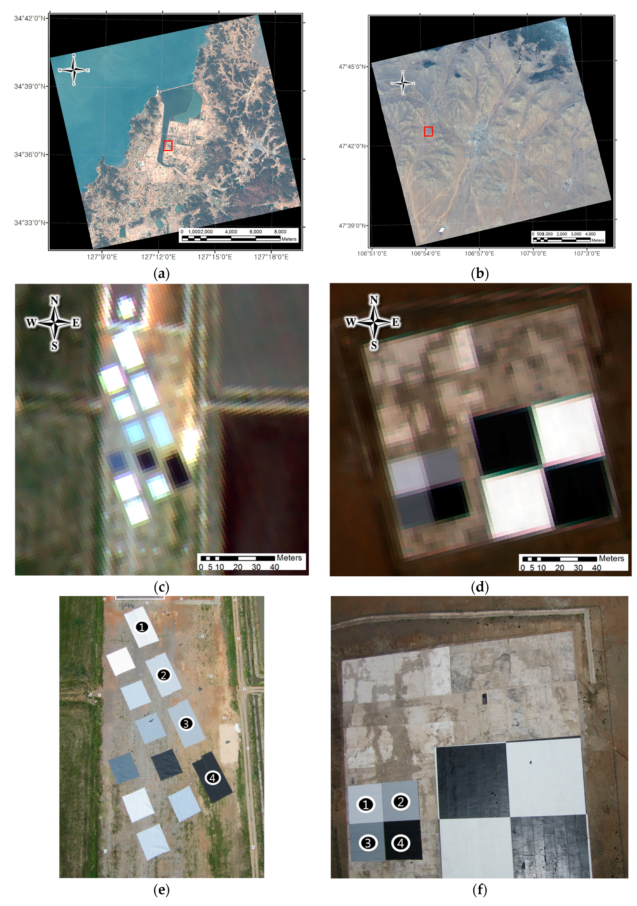
In this study, we selected two field campaign sites, Goheung (GH) County, South Korea (34.60°N, 127.20°E), and Zuunmod, Mongolia (MG) (47.721°N, 107.064°E). The locations of the field campaigns are shown in
Figure 1a,b. In the first field campaign at Goheung (
Figure 1a), we obtained cropped images of the tarp areas from the KOMPSAT-3A MS, and their corresponding unmanned aerial vehicle (UAV) images. These images are shown in
Figure 1c,e, respectively. We used the 10 × 20 m tarps numbered from one to four, shown to the right of
Figure 1e. We chose these over the smaller 10 × 10 m tarps to mitigate the PSF effects caused by the CCD camera [
18]. These can be reduced by increasing the spatial extent of the target. The 10 × 20 m tarps shown in
Figure 1c were represented by 5 × 10 pixel regions in the images. The edges, which were clearly influenced by the surrounding reflectance, are semitransparent. By visually inspecting these tarp areas, we can see that they are represented by areas of 3 × 8 pixels. Only pixels that were clearly part of the tarp area were used to determine the ground reference values for the KOMPSAT-3A DN. According to [
19], in order to obtain reasonable vicarious radiometric calibration results, the radiometric tarp must occupy an area of 5 × 5 pixels or more when observed from the satellite. The authors of that study used 20 × 20 m tarps to vicariously calibrate IKONOS satellites. The spatial resolution of the IKONOS satellites was 4 m. As the KOMPSAT-3A satellites have an MS channel spatial resolution of 2.2 m, areas represented by 5 × 5 pixels, which correspond to areas of 11 × 11 m or larger, can be used for vicarious calibration. The tarps used in the Goheung field observations were sufficiently large in the vertical direction, but 1 m too small in the horizontal direction. This made environmental effects more pronounced. In the second field campaign over Zuunmod (
Figure 1b,d,f), we used larger radiometric tarps with dimensions of 20 × 20 m, as shown in
Figure 1d,f. In
Figure 1d, we can see that the areas which are clearly tarps, occupy a minimum of 8 × 8 pixels in the KOMPSAT-3A MS images. Hence, for vicarious calibration, it is better to use larger radiometric tarps, like those used in the second field campaign. The observations of these tarps were less affected by the environment.
2.1. Schema of Vicarious Calibration Algorithm for KOMPSAT-3A Using 6S Radiative Transfer Model
In this study, we adopted the 6S radiative transfer model to simulate the physical radiance received by the KOMPSAT-3A MS sensor by retrieving the essential model input parameters. The 6S code, which is the improved version of 5S, includes a more accurate calculation of highly asymmetric aerosol scattering phase functions, arbitrary variation in the vertical aerosol profile, the ability to change the number of calculation angles and layers, and an increased number of node wavelengths from 10 to 20. The 6S radiative transfer model was validated by Kotchenova et al. [
21] and found to be consistent to within 1%, when compared with other RTMs [
22]. The model has been extensively validated, and its accuracy is stated to be within 1% [
23]. Therefore, securing accurate input parameters allows an exact atmospheric parameterization calculation, and it is imperative that such input parameters be considered and retained in order to estimate accurate DN-to-radiance coefficients. In this study, we improved the accuracy of the vicarious radiometric calibration algorithm by both improving the existing input data calculation method, and introducing a new method that was not used in the previous radiometric calibration study [
17].
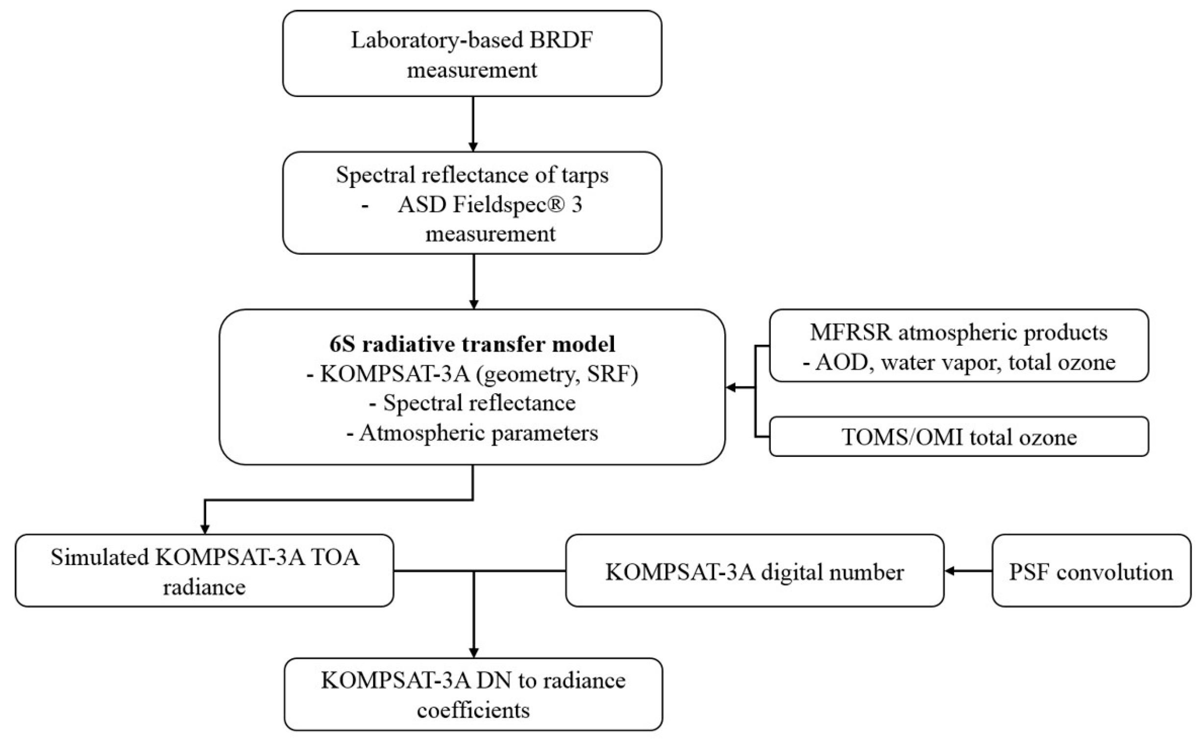
Figure 2 presents a flowchart of the vicarious radiometric calibration of KOMPSAT-3A using the 6S radiative transfer model and related input parameters. The main input parameter processes, such as the hyperspectral reflectance of tarps from ASD FieldSpec
® 3, laboratory-based BRDF measurements, precise atmospheric measurements from MFRSR, and PSF correction, were carefully applied to accurately calculate the amount of sensor-received radiance.
In addition, ancillary input parameters, such as geometric conditions, the spectral response function (SRF) for KOMPSAT-3A MS bands, and environmental surface reflectance, were also considered. To consider the background surface reflectance, we introduced an environmental function that models adjacency effects. This function takes into account the scattering effects induced by the difference in reflectance between the tarp and the surrounding area. We assumed that the surface reflectance was not uniform, as is the case with a circular target. In the 6S model, the adjacency effects were calculated based on the target reflectance, the target radius, and the environmental reflectance. We used surface spectral libraries from the Korean Institute of Geoscience and Mineral Resources (KIGAM) to determine the environmental reflectance. For more information, see the 6S radiative transfer model manual [
24].
Table 2 shows the KOMPSAT-3A geometric conditions for the vicarious radiometric calibration during the two field campaigns. Until we had acquired a useful KOMPSAT-3A calibration dataset, satisfying the clear-sky weather conditions and reliable geometric conditions with a viewing angle of less than 10 degrees, we had to command new observation orders for KOMPSAT-3A more than 10 times. During the IOT period, we finally acquired two calibratable KOMPSAT-3A images, with a viewing zenith angle of less than 10 degrees under clear-sky conditions. The first one was acquired on 27 May 2015 at 04:43 coordinated universal time (UTC), over Goheung, and the second was acquired on 18 June 2015 at 05:47 UTC, over Zuunmod (
Table 2).
Based on the size of the tarps at each location, we expected to observe reduced adjacency effects in the Zuunmod tarps, due to their ability to secure more purely reflected spectral reflectances compared to the first field campaign. Furthermore, the viewing zenith angle of KOMPSAT-3A during the Zuunmod field campaign was less than that of the first field campaign (see
Table 2), indicating that reduced effects of BRDF surface tarps and atmospheric loads could be expected.
2.2. ASD FieldSpec® 3 Measurements of the Hyperspectral Reflectance of Tarps
As mentioned previously, we deployed radiometric tarps before the expected KOMPSAT-3A pass time, as shown in
Figure 1e,f. To estimate the high-spectra resolution of the reference targets, we utilized an ASD FieldSpec
® 3 (ASD Inc., Boulder, CO, USA). This is a high-resolution spectroradiometer with a spectral resolution of 3 nm in the 350–1000 nm spectral range, and 10 nm in the 1000–2500 nm spectral range. The full spectral range of the spectroradiometer covers the KOMPSAT-3A MS bands (450–950 nm). Thus, the spectra of the radiometric tarps can be used as surface reference data. When performing ASD FieldSpec
® 3 measurements, it is important to use appropriate observation geometries and measurement times. To normalize the reflectance and reduce the BRDFs caused by the differences in the ASD FieldSpec
® 3 geometry and the changeable KOMPSAT-3A geometry [
25], we fixed the ASD observation geometry in the direction of the nadir. Then, we carefully measured the spectra of the radiometric tarps using the ASD FieldSpec
® 3. To reduce temporal observation discrepancies and the effects of changes in the solar zenith angle on the BRDF, we took these measurements in the hour before the KOMPSAT-3A passed over the tarps. When measuring the hyperspectral reflectance of the tarps using the ASD FieldSpec
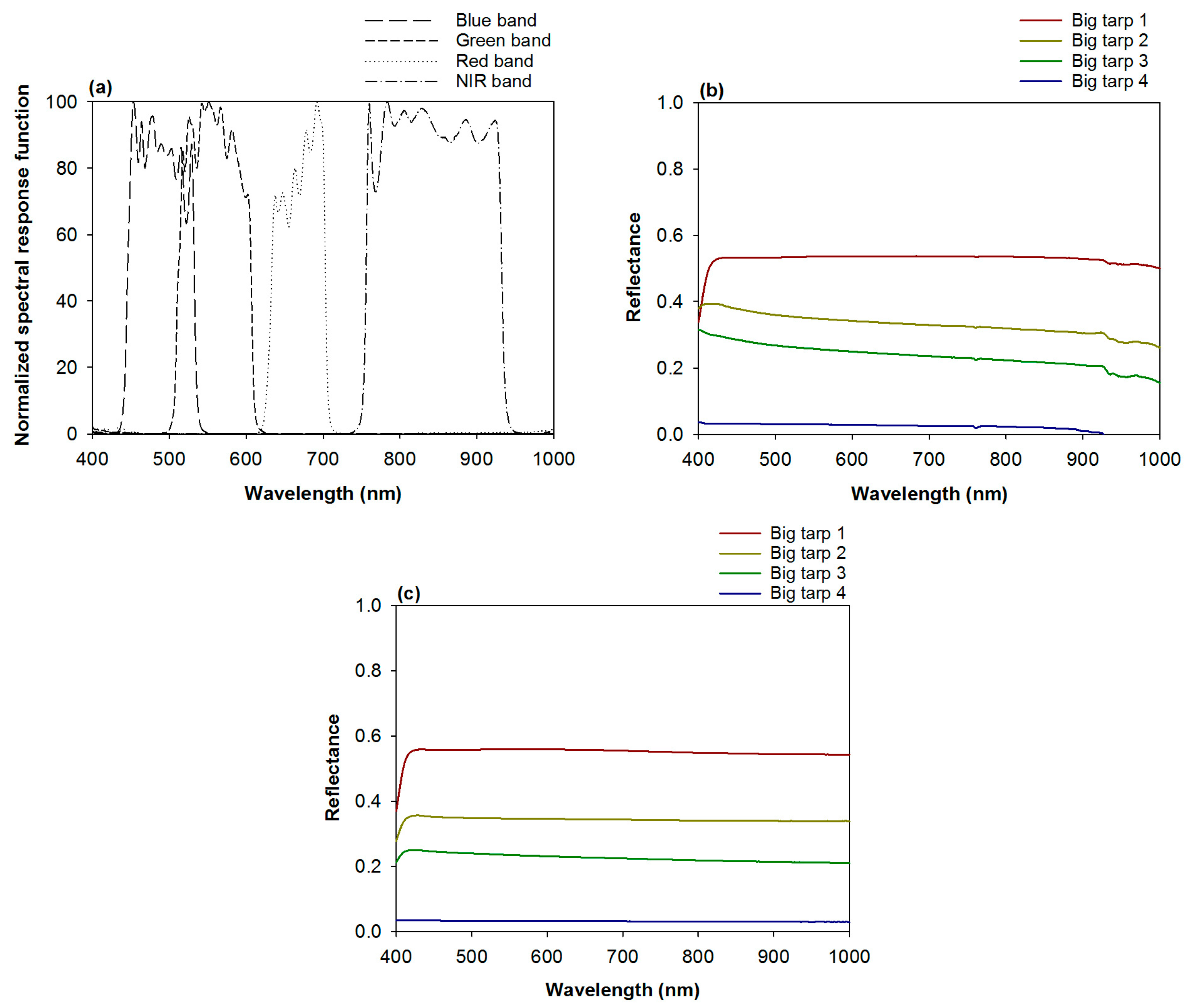
® 3, we ensured that the results reflected the spatial radiometric characteristics of the targets, by measuring points on each tarp at least 20 times, with 10 repetitions per measurement. The mean value of these measurements was used in simulations of the 6S model. The reflectance differed by less than 1% between any two points in each tarp. As shown in
Figure 3, all of the spectral reflectance curves of the four large tarps produced a spectrally flat pattern, with the exception of the starting points. As shown on the spectral curve, the reflectance of the radiometric tarps used in the second field campaign was constant over the spectral wavelength band. This indicates that the reflectances of the tarps measured at a resolution of 1 nm, could be used as reference surface values in simulations of the 6S radiative transfer model.
2.3. Laboratory-Based BRDF Measurements of Radiometric Tarps
The BRDF measurement is generally used to infer reflectance at a given viewing geometry and to compute a hemispheric albedo from a reflectance measurement made from a specific direction [
26]. The accuracy of such tarp-based field calibrations depends on an accurate knowledge of the tarps’ laboratory-measured BRDF at a variety of source illuminations and detector scatter angles [
27], as the BRDF effect is considered an unknown amount of error in the reflectance values [
28]. We performed laboratory-based BRDF measurements of the radiometric tarps to compensate for the observation discrepancy between nadir-direction ASD FieldSpec
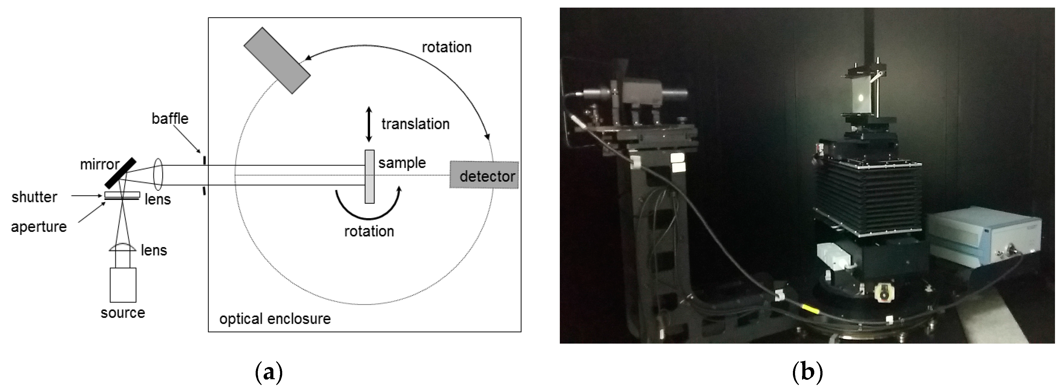
® 3 measurements, and solar target sensor-dependent KOMPSAT-3A geometry. First, we cut edge sections (30 cm × 30 cm) from each of the deployed radiometric tarps to measure BRDF in the laboratory. The radiometric tarp samples were made from chemically-treated canvas. We measured the BRDF characteristics of the deployed tarps according to the angle of incidence and reflection, using a hyperspectral gonioreflectometer designed to measure two-dimensional BRDFs for the principal plane. The hyperspectral gonioreflectometer consists of a source system and a goniometric detection system, as shown in
Figure 4 [
29]. The source system has dual sources: a Xe lamp emitting wavelengths in the 380–780 nm range, and a super-continuum laser emitting wavelengths in the 450–1000 nm range. As its wavelength range covered the spectral bands of the KOMPSAT-3A AEISS-A sensors, the super-continuum laser source was used for the BRDF measurements. The beam was adjusted with two lenses and an aperture, and then directed toward the sample. The goniometric detection system had a central axis with two-rotational stages, one for the sample and one for the detection system. We used a three-axis translational stage to adjust the position of the sample and the sample plane to the central axis. The detection system had an aperture that was used to define the solid angle of detection in the reflected radiance measurements, and a fiber-optic probe connected to a CCD-based spectroradiometer with a bandwidth of 3 nm. The instrument used an absolute method to measure the BRDF: the incident irradiance was measured with the sample translated away from the beam path, and the detection system positioned along the beam path. To measure the reflected radiance, the sample was positioned in the beam path, and the detection system was positioned at the angle of reflection.
Based on the laboratory BRDF measurements, anisotropy factors (ANIFs) of each radiometric tarp were estimated using the following equation [
28]:
where
is the BRDF for illumination radiance that comes from elevation (
) directions, which is reflected to elevation directions (
) at wavelength
in the principal plane. Basically,
was intended for the BRDF measurement of KOMPSAT-3A geometry for the Goheung and Zuunmod field campaigns.
BRDFN(
φi,
θi;
φr,
θN;
λ), which corresponds to the nadir-direction-measured ASD FieldSpec
® 3 result, is measured in the nadir direction (
= 0°). The ANIF is an intuitive reflectance anisotropy measure that varies in theory between 0 and
[
30].
The values for each of the field campaign geometries are estimated to normalize the MS reflectance of KOMPSAT-3A to the nadir direction, corresponding to the ASD FieldSpec
® 3 observation based on following equation:
where
is the normalized MS reflectance of KOMPSAT-3A in the nadir direction, and
is the original reflectance of KOMPSAT-3A for the instantaneous geometry conditions in
Table 2. In previous studies [
17], laboratory-based BRDF measurements have been made and directional uncertainties for radiometric tarps were calculated, but no corrections were made for actual KOMPSAT-3 images. In the previous study, the solar zenith angle and the viewing zenith angle were measured at 10 degree intervals. Due to errors in the process used to interpolate between the intervals, only the uncertainty due to measurements of the tarp was shown. In this study, we used actual KOMPSAT-3A geometric conditions, shown in
Table 2, to correct for the fact that we were using satellite images.
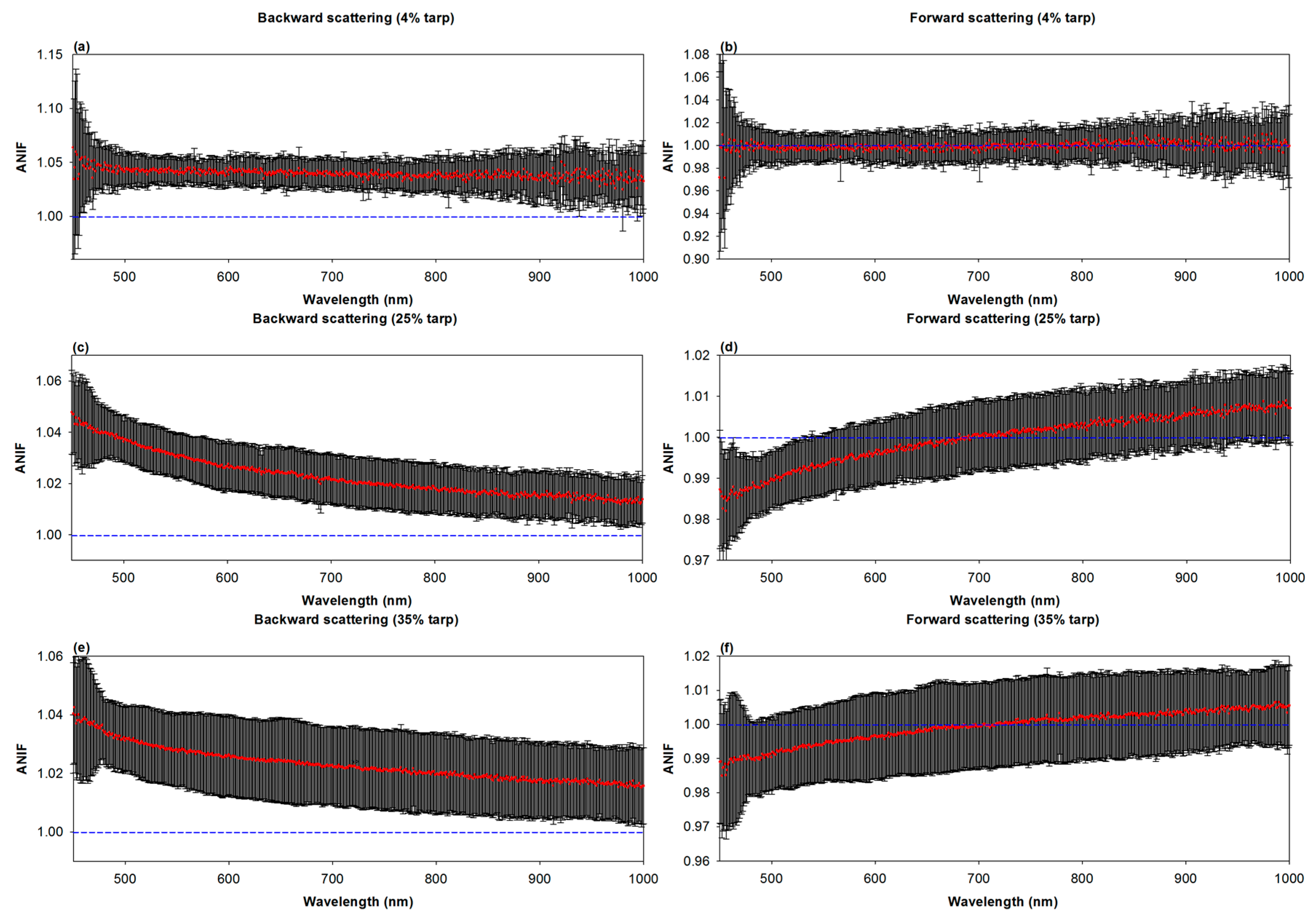
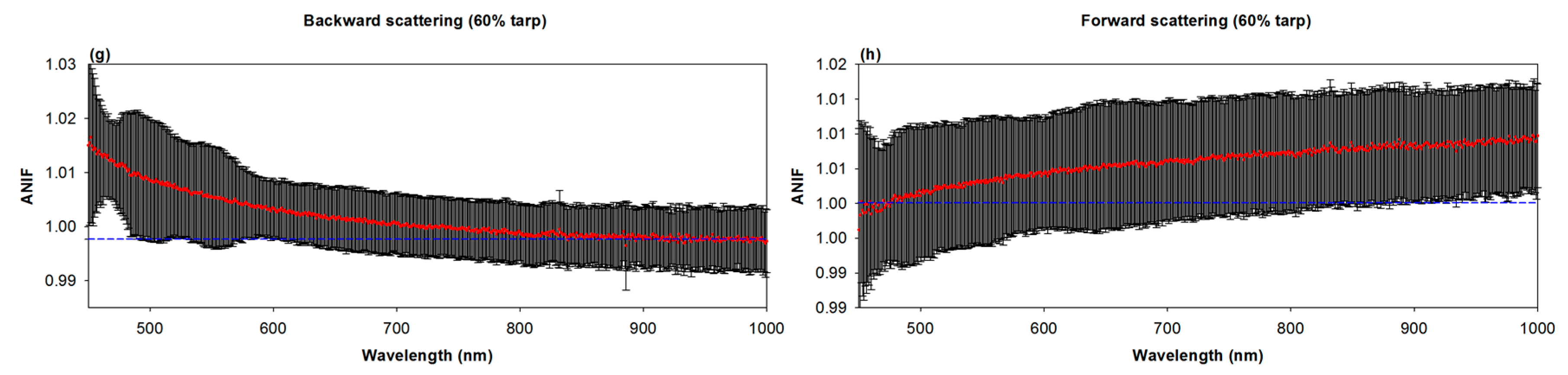
Figure 5 and
Figure 6 show the estimated ANIF values according to each radiometric tarp (from 4% to 60% reflectance), obtained by reflecting the geometries of the Goheung and Zuunmod field campaigns, respectively. For example, in
Figure 5, for estimating ANIF, the laboratory-based BRDF measurement geometry condition is 21.3° incidence with ±9.9° detection (negative is backward scattering and positive is forward scattering), which is the same as the satellite observation geometry for the Goheung field campaign. In
Figure 6, the experiment geometry condition is 26.6° incidence with ±2.9° detection, the same as the Zuunmod field campaign. As shown in
Figure 5, we found slightly inverse symmetrical patterns of ANIF values for all radiometric tarps, except for the 4% tarp, indicating two important facts. The first is that the changeable sun–tarp–sensor geometry should be considered, in order to determine which scattering phases would be reflected by checking geometrical conditions. The second is that radiometric tarps would be expected to have effects on BRDF values in the azimuth direction. We inferred that the inverse symmetry of BRDF values between backward and forward scattering originated from the dependence of the tarps’ weft and warp thread orientations on the diffuse reflectance [
27]. Under backward scattering conditions, the ANIF values, and even the uncertainties, deviated from 1, except for the 60% tarp, which approached 1 as the wavelength increased (
Figure 5a,c,e,g). This means that the effects of the radiometric tarps on BRDF are more effective for shortwave ranges, such as the blue and green bands. In the case of forward scattering, not only were ANIF values near 1, but an ANIF value of 1 was included in the uncertainty range over most of the measurement wavelengths (
Figure 5b,d,f,h). For the Goheung field campaign site (
Table 2), the ANIF value for backward scattering was applied, in order to normalize the satellite reflectance, because the relative azimuth angle between satellites and the sun is 25.4°.
In the case of the Zuunmod field campaign, because the site has a decreased viewing zenith angle (detection angle) compared to the Goheung site, weaker BRDF effects, which are sensitive to the extent of off-nadir direction, would be expected. Therefore, inevitably, the ANIF values and the uncertainties were near 1, indicating that the radiometric tarps of the Zuunmod field campaign with a +2.9° viewing zenith angle, have weak effects on the BRDF.
We only applied ANIF-based correction for the Goheung site, based on the laboratory BRDF measurements using Equation (2).
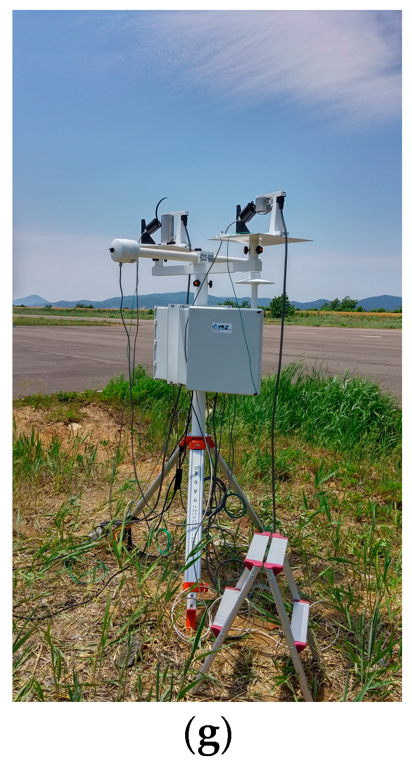
2.4. Atmospheric Conditions Using MFRSR for AOD and Column Water Vapor
In this study, we used MFRSR observation equipment to obtain accurate atmospheric data. In our previous study, we used less accurate MODIS equipment, so the uncertainty in our measurements was higher [
17]. The MFRSR has been used to measure atmospheric parameters, such as AOD and water vapor [
31,
32]. For the atmospheric parameterization, MFRSR-measured AOD and column water vapor were used as input parameters to derive sensor-level radiance.
In the case of AOD estimation with MFRSR, we first measured the total, direct, and diffuse irradiances at the Goheung and Zuunmod field campaign sites. In general, the well-known Langley regression method is widely used to estimate AOD by retrieving the TOA irradiance (I
0), by securing at least two months of continuous measurements that are long enough to reduce the statistical variability to less than 1% per day [
33]. However, it is difficult to acquire long-term continuous observations during vicarious calibration field campaign periods. In this study, to overcome this limitation of the Langley regression method, the modified Langley correction method, using the maximum value composite (MVC) of the largest irradiance values at a given air mass, was applied. Lee et al. [
34] proved that the suggested MVC-based Langley method (hereafter, Langley
MVC) showed reasonable statistical results for nearly impossible-to-find days that meet the requirements for performing traditional Langley analyses.
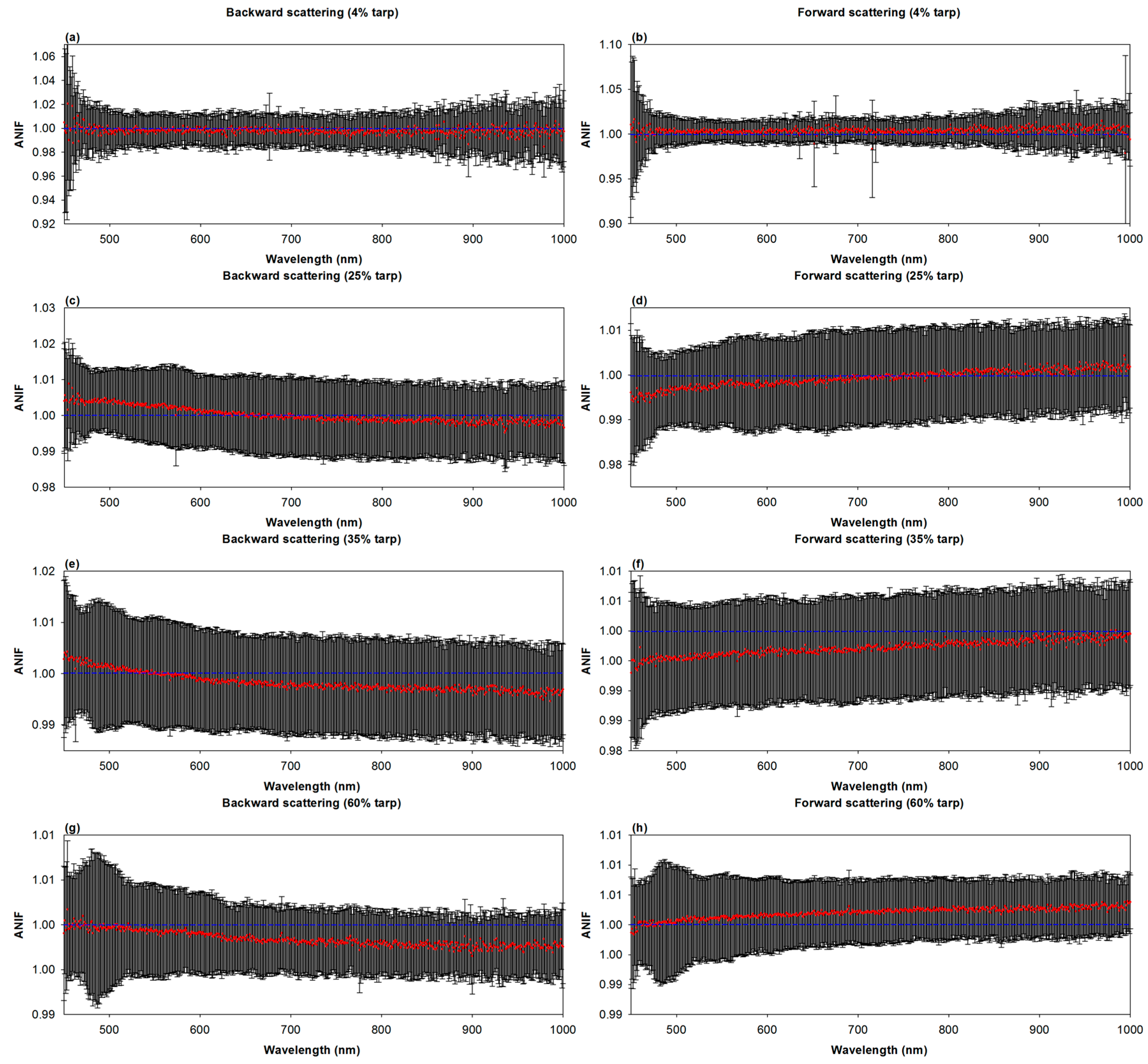
Figure 7 shows an example of the Langley plots of the MFRSR 496 nm channel irradiance data as functions of air mass, for Goheung and Zuunmod. The Langley
MVC cannot deal with temporal changes in I
0 during a given composite period; therefore, the smoothing and removal of outliers using a filtering technique were employed from one composite period to another [
35]. The correlation coefficients for Goheung and Zuunmod were 0.996 and 0.982, respectively, indicating that the I
0 from Langley
MVC would be useful for deriving the total optical depth (TOD) during the field campaigns.
Based on the
determined from Langley
MVC, TOD (
) was estimated using the following equation:
where
is the instantaneous direct solar irradiance from the MVC method and m is the air mass. The TOD during any time of the day consisted of the Rayleigh optical depth (ROD,
), AOD (
), and gas absorption optical depth (GAOD,
), as follows:
Therefore, AOD can be derived by subtracting ROD and GAOD, from TOD. ROD can be calculated as a function of wavelength (
) [
36], as follows:
Although gas absorption is effectively zero for many regions of the solar spectrum, ozone absorption at the 496, 615, and 670 nm wavelengths, and NO
2 absorption at the 415, 496, and 615 nm MFRSR wavelength channels, are sensitive [
33,
37], and must be taken into account. Therefore, the optical depths of ozone absorption and NO
2 absorption were estimated using the corresponding ozone absorption coefficients [
38] and NO
2 absorption cross-sections [
39], following Equations (6) and (7), respectively:
where
in cm
−1 is the ozone absorption coefficient and
DO3 is the total column ozone in Dobson units (DU) from the Total Ozone Mapping Spectrometer (TOMS) instrument and the Ozone Monitoring Instrument (OMI). Similarly, total column NO
2 (
) from the OMI was used to derive NO
2 absorption (
). In this study, we used the TOMS OMI total ozone as the input parameter for the 6S model to simulate ozone absorption.
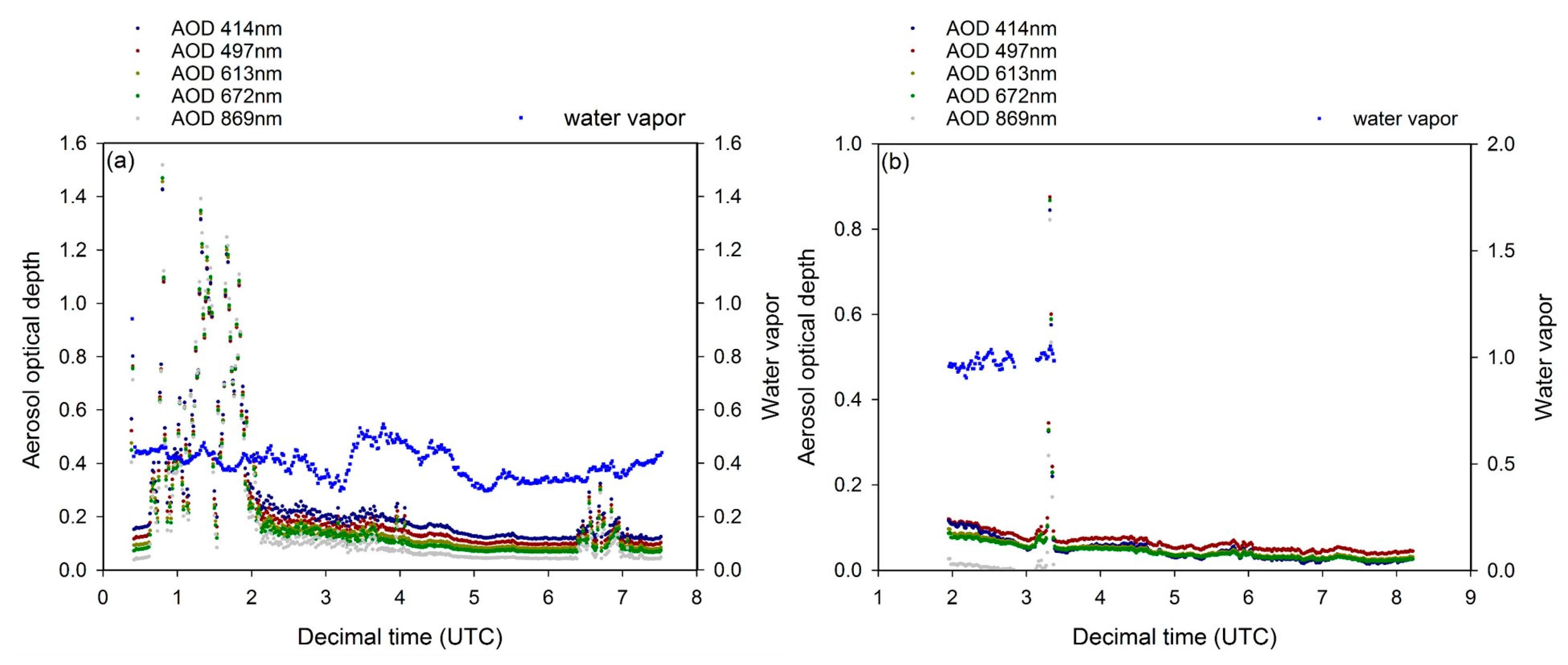
Figure 8 shows the final results of MFRSR AOD over Goheung and Zuunmod. The scattered patterns of Goheung in the morning were caused by passing clouds, according to visual inspection of Geostationary Ocean Color Imager (GOCI) RGB images. Afterwards, all spectral channels showed stable AOD curves. The Zuunmod field campaign site showed more stable AOD curves and longer periods of clear skies. For both sites, the estimated AODs could be used as an input parameter of the 6S radiative transfer model.
Among the seven MFRSR channels, the 937 nm channel is used to derive the water vapor optical depth (WVOD,
). In the derivation of WVOD, Equation (3) is expressed as Equation (8), because other gaseous absorptions are negligible and water vapor absorption is strong at this wavelength:
WVOD can be expressed as Equation (9), denoting the column water vapor and including the optical pass length by water vapor (
), and constants a and b [
32]:
In the case of the Zuunmod field campaign, a discontinuous pattern was found after 3:00 UTC, because unrealistic TOD values were recorded. According to the MFRSR measurements of Zuunmod, stable clear skies were detected, indicating that we can select the value for water vapor at the time closest to the KOMPSAT-3A passing time, by assuming that the variation in column water vapor is insignificant.
Table 3 shows selected values for AOD, water vapor, and ozone at satellite overpass times, for the Goheung and Zuunmod sites.
2.5. Retrieval of PSF with KOMPSAT-3A MS Bands by Observing Stars
The PSF, which is the electronic response of a sensor system to a point radiator, is an important criterion of image quality [
40]. How well the PSF is defined is also important, as the PSF of the CCD camera can seriously affect the accuracy of radiometric calibration and measurement [
41]. In addition, the impact of the PSF on the optical sensor results in considerable uncertainties in derived MODIS land cover products [
42]. Therefore, we also newly considered the effects of the PSF by observing images of a point source, such as a bright star, to characterize the AEISS-A sensor response to the point source [
43,
44]. We observed stars using KOMPSAT-3A MS to measure the PSF of the AEISS-A sensor during the IOT periods. The satellite attitude control system can be used to observe stars by rotating KOMPSAT-3A during Eclipse orbits. To select an effective bright star source, we first eliminated background noise, and then applied a threshold value by considering a high signal-to-noise ratio (SNR) and an unsaturated DN value. To select stars with radiances within the detection range of AEISS-A, we referred to the Gunn & Stryker Stellar spectrophotometric atlas, which contains information on the visible spectra of 175 stars [
45].
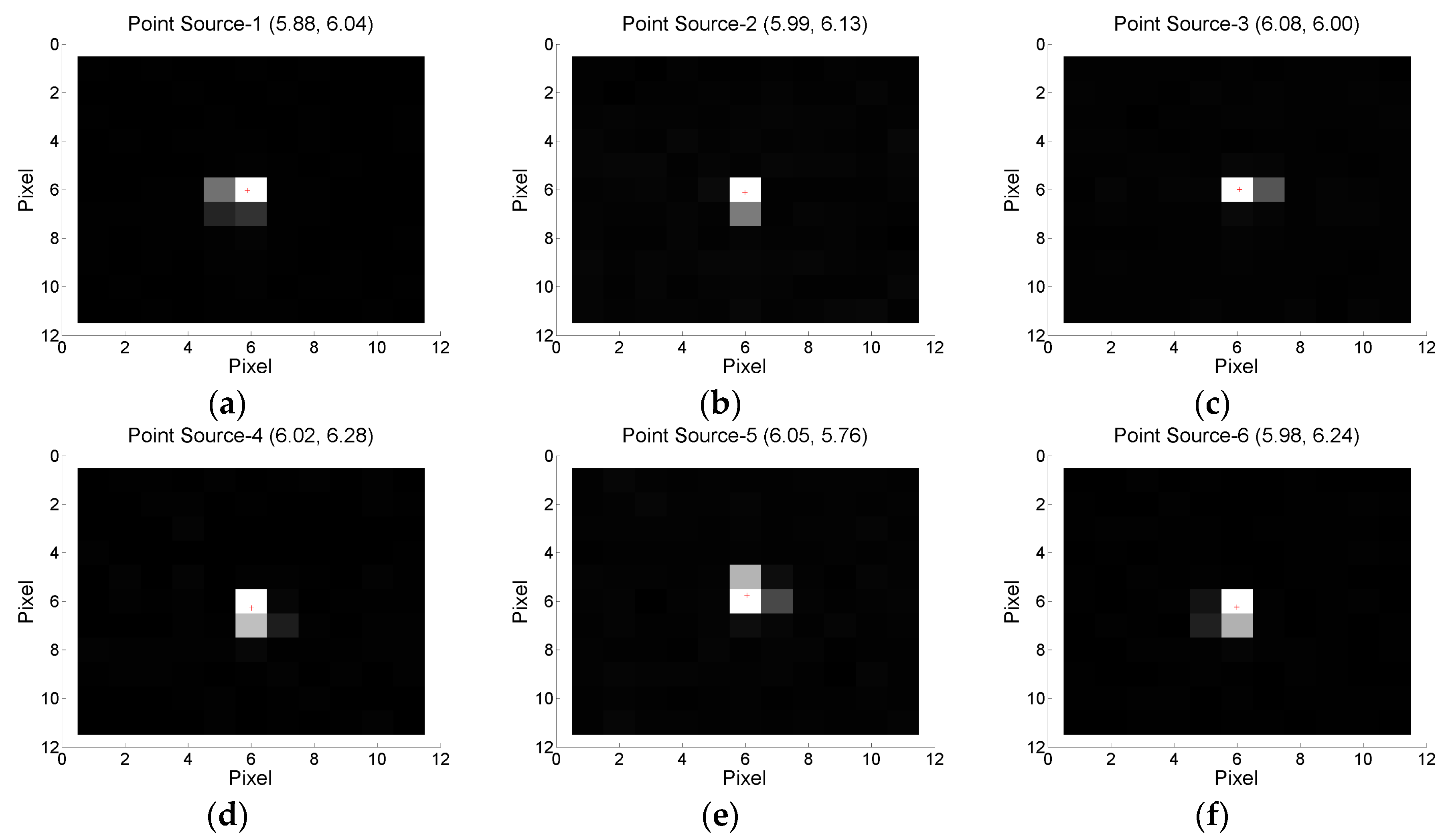
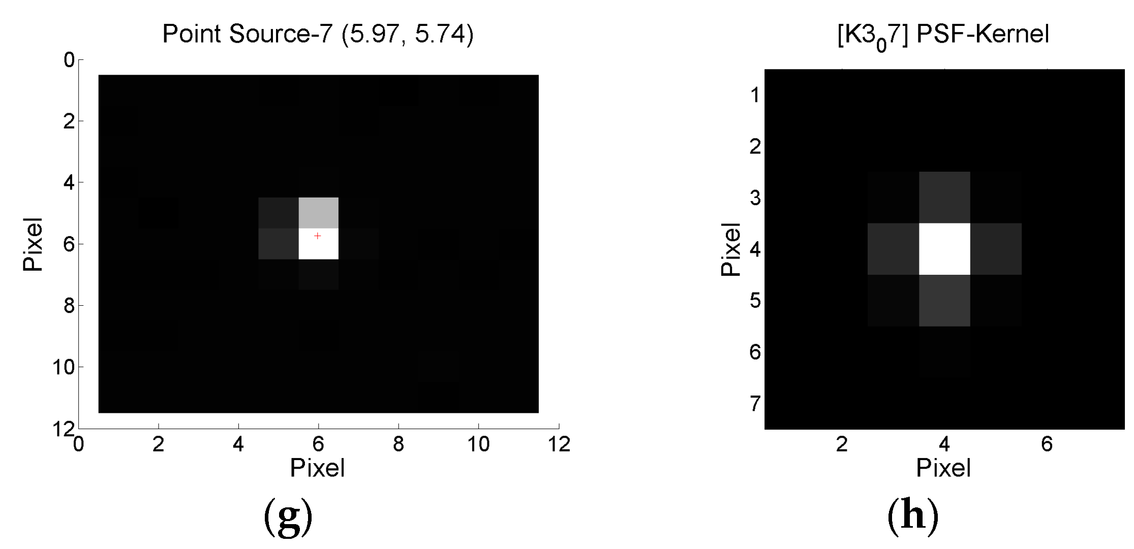
Figure 9 shows measured star images from the KOMPSAT-3A-combined MS bands.
Figure 9h shows the overlaid KOMPSAT-3A MS images of selected stars, and the highest points of the images are the locations of the stars. Based on
Figure 9h, 3 × 3 pixels were the sensitive area for PSF effects, indicating that the adjacency effects can be reduced and PSF compensated for, by using tarps that are large enough, such as those occupying 5 × 5 pixels (11 × 11 m in the nadir direction in the KOMPSAT-3A MS images) or more.
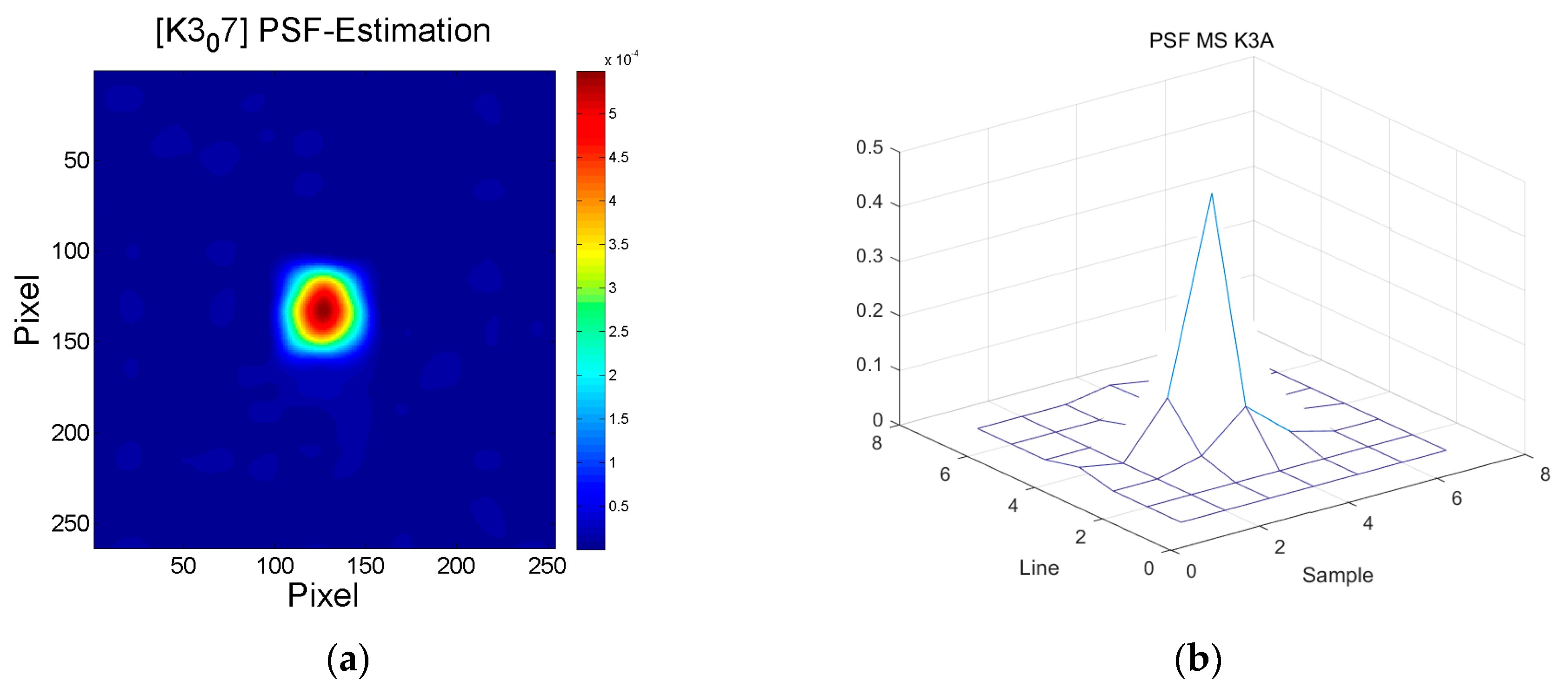
To reduce the diffraction effects by AEISS-A CCD sensor characteristics, the PSF of the KOMPSAT-3A MS was generated from the star image data acquired by the MS bands of KOMPSAT-3A.
Figure 10a shows the observed PSF of KOMPSAT-3A AEISS-A, as a function of radius at 25% full width and half maximum (FWHM). Although not a circle, the shape of the PSF is similar to a circularly symmetric Gaussian-like shape. Then, converting the matrix of the PSF based on star observations, the optical transfer function (OTF) of the system was simulated by Fourier transformation of the simulated PSF in
Figure 10b. The MTF of KOMPSAT-3A MS was determined by the magnitude of calculated OTF.
Finally, by dividing the Fourier-transformed KOMPSAT-3A MS image in the frequency domain by the determined MTF, we calculated the satellite image data compensating for the PSF effect. The focusing system of the AEISS-A mainly depended on the temperature of the sensor focal lens, as we did not consider that the PSF change caused the temperature of the sensor focal lens, because its variation is nonlinear.


