
Validation of Spaceborne and Modelled Surface Soil Moisture Products with Cosmic-Ray Neutron Probes

 ,
,  ,
, 
Abstract
:
1. Introduction
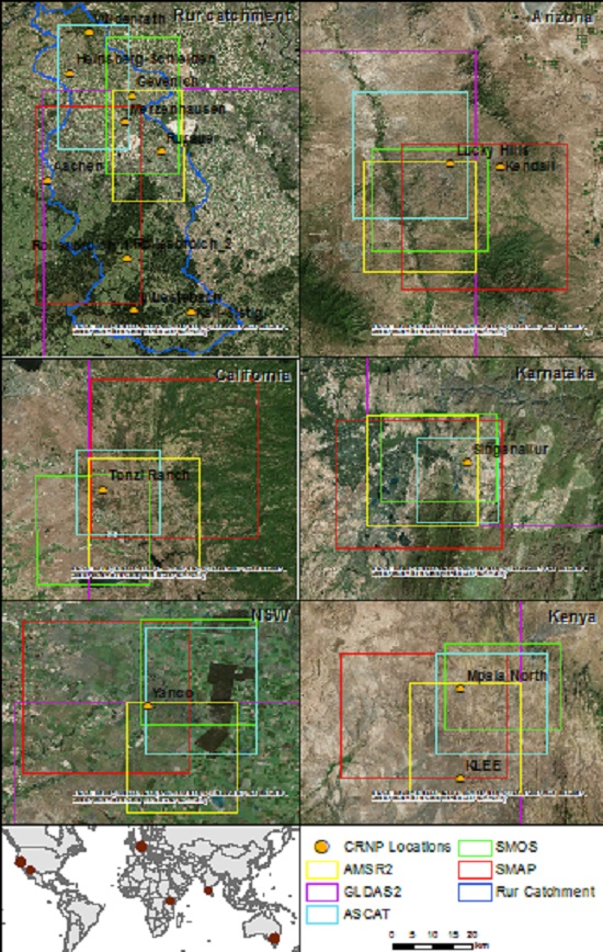
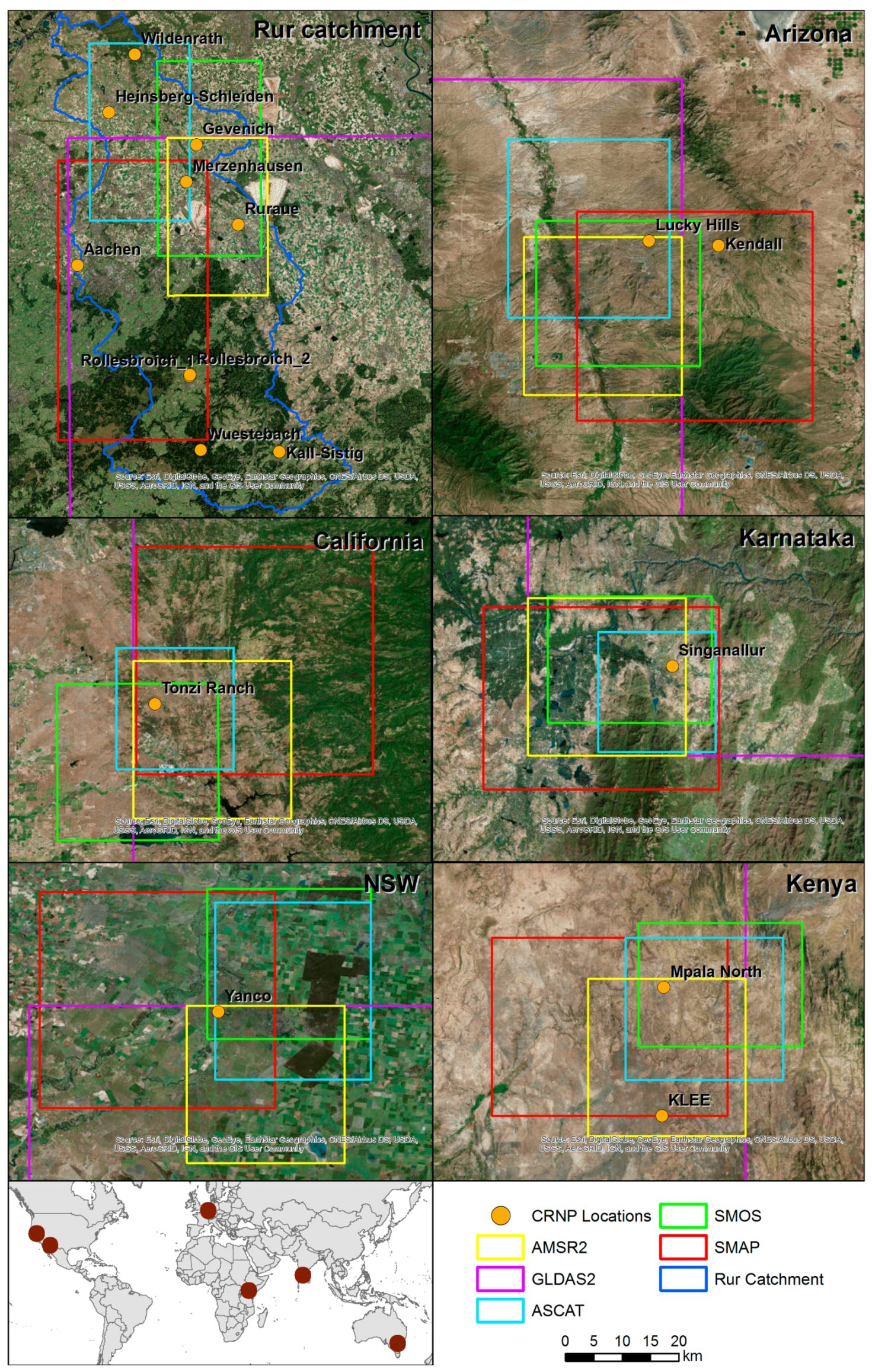
2. Test Regions
2.1. TERENO Site Rur Catchment
2.2. Walnut Gulch, Arizona, USA
2.3. Tonzi Ranch, California, USA
2.4. CosmOz Site New South Wales, Australia
2.5. COSMOS Sites Kenya
2.6. Karnataka, India
3. Soil Moisture Data Sets
3.1. AMSR-2
3.2. ASCAT
3.3. SMAP
3.4. SMOS
3.5. GLDAS2-NOAH
3.6. Cosmic-Ray Neutron Probes
4. Description of the Metrics Used for Validation
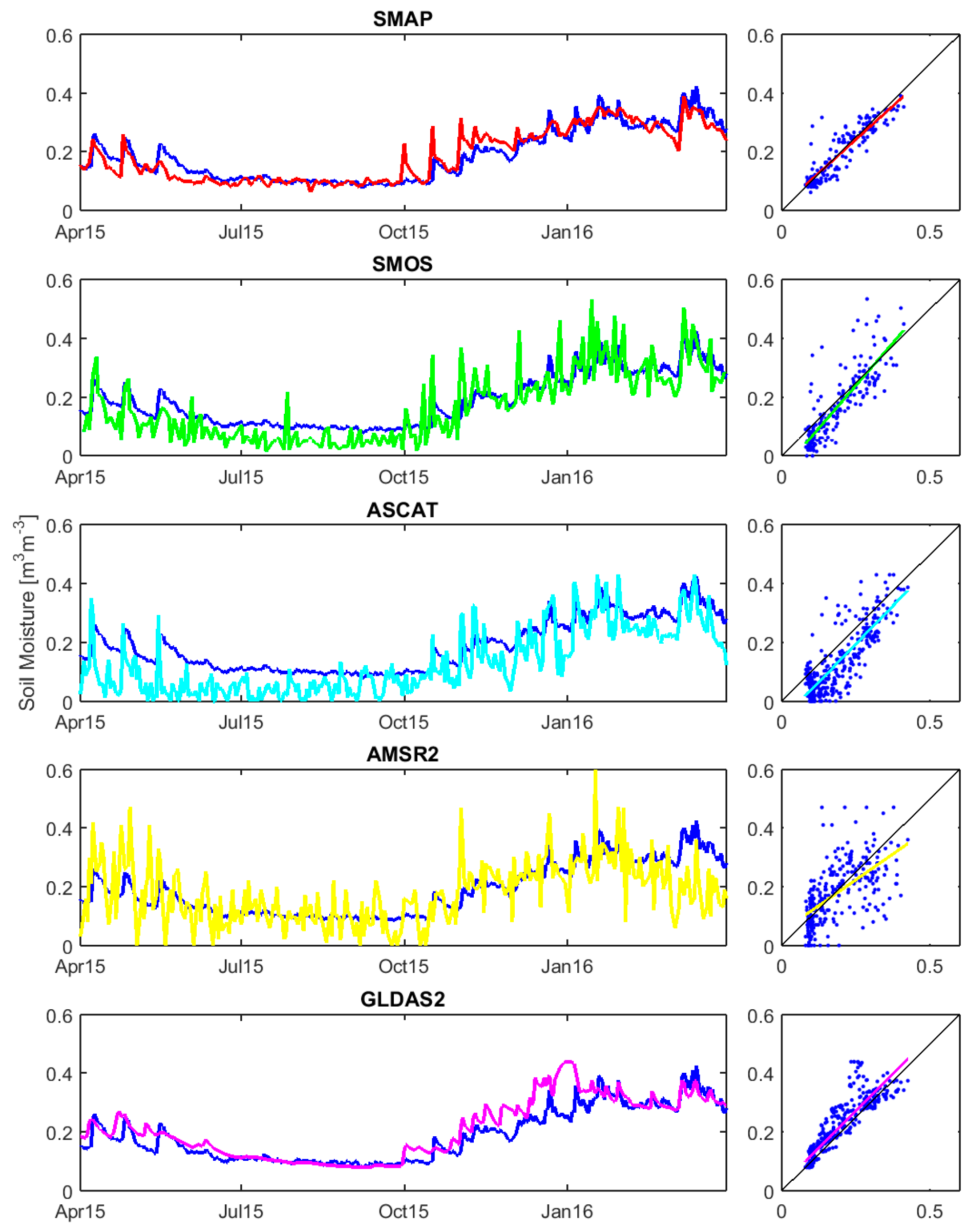
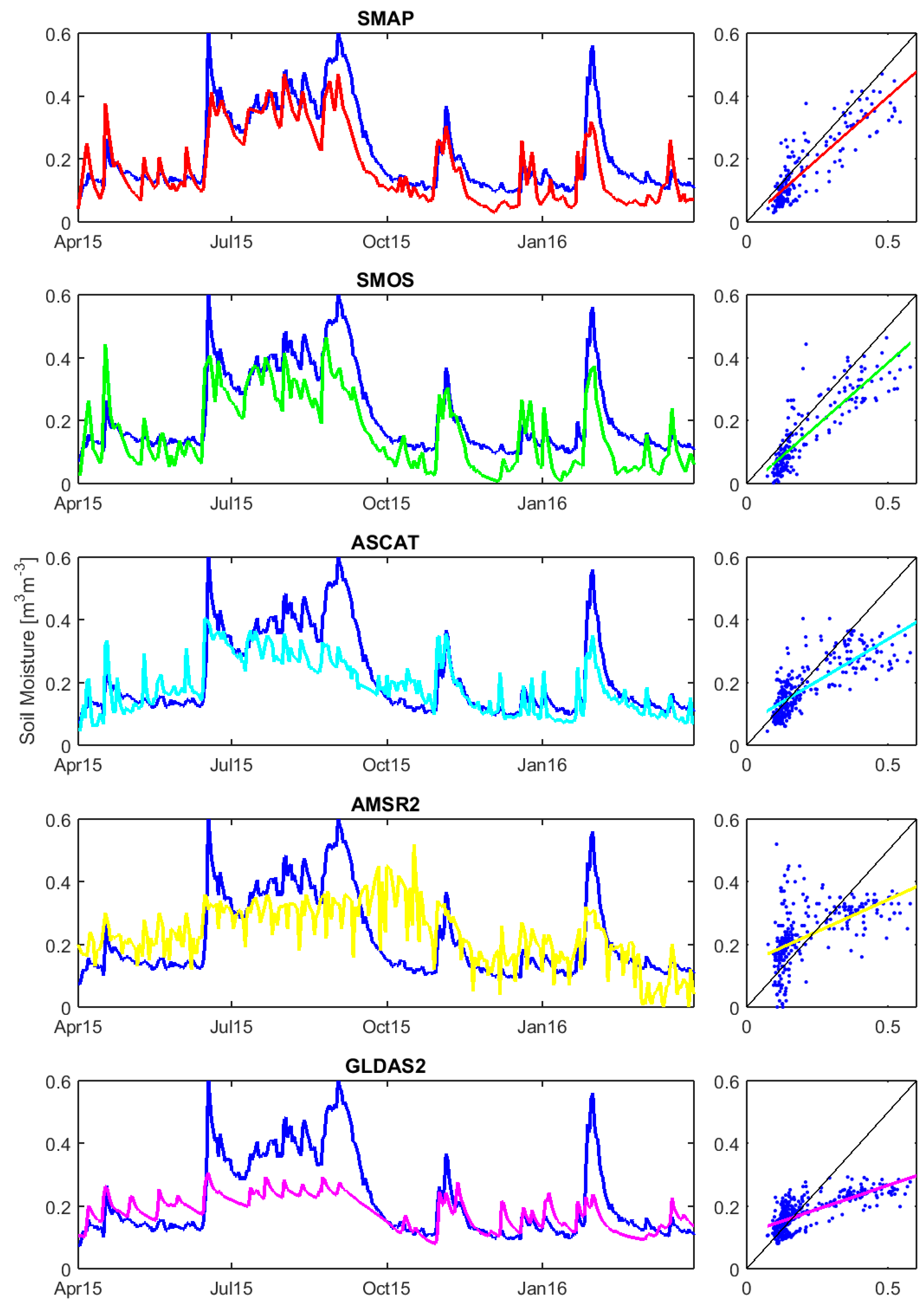
5. Results and Discussion
5.1. Standard Metrics
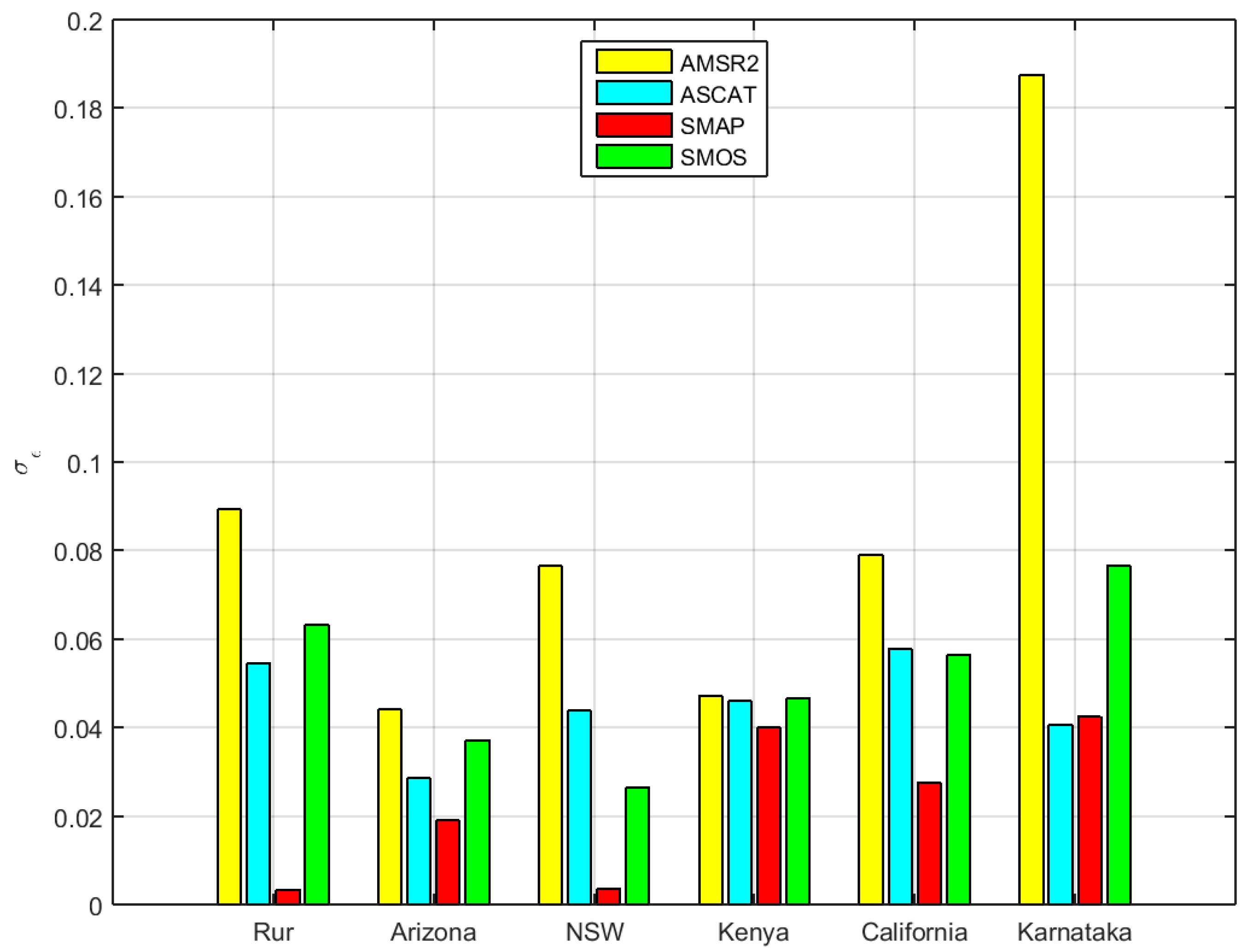
5.2. Triple Collocation Results
6. Conclusions and Outlook
Acknowledgments
Author Contributions
Conflicts of Interest
References
- Vereecken, H.; Huisman, J.A.; Pachepsky, Y.; Montzka, C.; van der Kruk, J.; Bogena, H.; Weihermüller, L.; Herbst, M.; Martinez, G.; Vanderborght, J. On the spatio-temporal dynamics of soil moisture at the field scale. J. Hydrol. 2014, 516, 76–96. [Google Scholar] [CrossRef]
- Vereecken, H.; Schnepf, A.; Hopmans, J.W.; Javaux, M.; Or, D.; Roose, T.; Vanderborght, J.; Young, M.H.; Amelung, W.; Aitkenhead, M.; et al. Modeling soil processes: Review, key challenges, and new perspectives. Vadose Zone J. 2016, 15, 57. [Google Scholar] [CrossRef]
- Kerr, Y.H. Soil moisture from space: Where are we? Hydrogeol. J. 2007, 15, 117–120. [Google Scholar] [CrossRef]
- Simmer, C.; Thiele-Eich, I.; Masbou, M.; Amelung, W.; Bogena, H.; Crewell, S.; Diekkruger, B.; Ewert, F.; Franssen, H.J.H.; Huisman, J.A.; et al. Monitoring and modeling the terrestrial system from pores to catchments the transregional collaborative research center on patterns in the soil-vegetation-atmosphere system. Bull. Am. Meteorol. Soc. 2015, 96, 1765–1787. [Google Scholar] [CrossRef]
- Wanders, N.; Karssenberg, D.; de Roo, A.; de Jong, S.M.; Bierkens, M.F.P. The suitability of remotely sensed soil moisture for improving operational flood forecasting. Hydrol. Earth Syst. Sci. 2014, 18, 2343–2357. [Google Scholar] [CrossRef]
- Sheffield, J.; Wood, E.F.; Chaney, N.; Guan, K.Y.; Sadri, S.; Yuan, X.; Olang, L.; Amani, A.; Ali, A.; Demuth, S.; et al. A drought monitoring and forecasting system for Sub-Sahara African water resources and food security. Bull. Am. Meteorol. Soc. 2014, 95, 861–882. [Google Scholar] [CrossRef]
- Seneviratne, S.I.; Corti, T.; Davin, E.L.; Hirschi, M.; Jaeger, E.B.; Lehner, I.; Orlowsky, B.; Teuling, A.J. Investigating soil moisture-climate interactions in a changing climate: A review. Earth-Sci. Rev. 2010, 99, 125–161. [Google Scholar] [CrossRef]
- Wagner, W.; Bloschl, G.; Pampaloni, P.; Calvet, J.C.; Bizzarri, B.; Wigneron, J.P.; Kerr, Y. Operational readiness of microwave remote sensing of soil moisture for hydrologic applications. Nord. Hydrol. 2007, 38, 1–20. [Google Scholar] [CrossRef]
- Mohanty, B.P.; Cosh, M.; Lakshmi, V.; Montzka, C. Soil moisture remote sensing—State-of-the-science. Vadose Zone J. 2017, in press. [Google Scholar]
- Entekhabi, D.; Njoku, E.G.; O’Neill, P.E.; Kellogg, K.H.; Crow, W.T.; Edelstein, W.N.; Entin, J.K.; Goodman, S.D.; Jackson, T.J.; Johnson, J.; et al. The soil moisture active passive (SMAP) mission. Proc. IEEE 2010, 98, 704–716. [Google Scholar] [CrossRef]
- Kerr, Y.H.; Waldteufel, P.; Wigneron, J.P.; Delwart, S.; Cabot, F.; Boutin, J.; Escorihuela, M.J.; Font, J.; Reul, N.; Gruhier, C.; et al. The smos mission: New tool for monitoring key elements of the global water cycle. Proc. IEEE 2010, 98, 666–687. [Google Scholar] [CrossRef]
- Bartalis, Z.; Wagner, W.; Naeimi, V.; Hasenauer, S.; Scipal, K.; Bonekamp, H.; Figa, J.; Anderson, C. Initial soil moisture retrievals from the METOP-A Advanced Scatterometer (ASCAT). Geophys. Res. Lett. 2007, 34. [Google Scholar] [CrossRef]
- Wagner, W.; Hahn, S.; Kidd, R.; Melzer, T.; Bartalis, Z.; Hasenauer, S.; Figa-Saldana, J.; de Rosnay, P.; Jann, A.; Schneider, S.; et al. The ASCAT soil moisture product: A review of its specifications, validation results, and emerging applications. Meteorol. Z. 2013, 22, 5–33. [Google Scholar]
- Parinussa, R.M.; Holmes, T.R.H.; Wanders, N.; Dorigo, W.A.; de Jeu, R.A.M. A preliminary study toward consistent soil moisture from amsr2. J. Hydrometeorol. 2015, 16, 932–947. [Google Scholar] [CrossRef]
- Bindlish, R.; Jackson, T.J.; Gasiewski, A.J.; Klein, M.; Njoku, E.G. Soil moisture mapping and AMSR-E validation using the PSR in SMEX02. Remote Sens. Environ. 2006, 103, 127–139. [Google Scholar] [CrossRef]
- Bosch, D.D.; Lakshmi, V.; Jackson, T.J.; Choi, M.; Jacobs, J.M. Large scale measurements of soil moisture for validation of remotely sensed data: Georgia soil moisture experiment of 2003. J. Hydrol. 2006, 323, 120–137. [Google Scholar] [CrossRef]
- Magagi, R.; Berg, A.A.; Goita, K.; Belair, S.; Jackson, T.J.; Toth, B.; Walker, A.; McNairn, H.; O’Neill, P.E.; Moghaddam, M.; et al. Canadian experiment for soil moisture in 2010 (CanEx-SM10): Overview and preliminary results. IEEE Trans. Geosci. Remote Sens. 2013, 51, 347–363. [Google Scholar] [CrossRef]
- Montzka, C.; Bogena, H.R.; Weihermüller, L.; Jonard, F.; Bouzinac, C.; Kainulainen, J.; Balling, J.E.; Loew, A.; Dall’Amico, J.T.; Rouhe, E.; et al. Brightness temperature and soil moisture validation at different scales during the smos validation campaign in the rur and erft catchments, Germany. IEEE Trans. Geosci. Remote Sens. 2013, 51, 1728–1743. [Google Scholar] [CrossRef]
- dall’Amico, J.T.; Schlenz, F.; Loew, A.; Mauser, W. First results of SMOS soil moisture validation in the upper Danube catchment. IEEE Trans. Geosci. Remote Sens. 2012, 50, 1507–1516. [Google Scholar] [CrossRef]
- Bircher, S.; Balling, J.E.; Skou, N.; Kerr, Y.H. Validation of smos brightness temperatures during the hobe airborne campaign, western Denmark. IEEE Trans. Geosci. Remote Sens. 2012, 50, 1468–1482. [Google Scholar] [CrossRef]
- Schlenz, F.; dall’Amico, J.T.; Loew, A.; Mauser, W. Uncertainty assessment of the smos validation in the upper Danube catchment. IEEE Trans. Geosci. Remote Sens. 2012, 50, 1517–1529. [Google Scholar] [CrossRef]
- Peischl, S.; Walker, J.P.; Ryu, D.; Kerr, Y.H.; Panciera, R.; Rudiger, C. Wheat canopy structure and surface roughness effects on multiangle observations at L-band. IEEE Trans. Geosci. Remote Sens. 2012, 50, 1498–1506. [Google Scholar] [CrossRef]
- Wigneron, J.P.; Schwank, M.; Baeza, E.L.; Kerr, Y.; Novello, N.; Millan, C.; Moisy, C.; Richaume, P.; Mialon, A.; Al Bitar, A.; et al. First evaluation of the simultaneous SMOS and ELBARA-II observations in the mediterranean region. Remote Sens. Environ. 2012, 124, 26–37. [Google Scholar] [CrossRef]
- Panciera, R.; Walker, J.P.; Jackson, T.J.; Gray, D.A.; Tanase, M.A.; Ryu, D.; Monerris, A.; Yardley, H.; Rudiger, C.; Wu, X.L.; et al. The soil moisture active passive experiments (SMAPEx): Toward soil moisture retrieval from the SMAP mission. IEEE Trans. Geosci. Remote Sens. 2014, 52, 490–507. [Google Scholar] [CrossRef]
- Colliander, A.; Jackson, T.; McNairn, H.; Chazanoff, S.; Dinardo, S.; Latham, B.; O’Dwyer, I.; Chun, W.; Yueh, S.; Njoku, E. Comparison of airborne passive and active L-band system (PALS) brightness temperature measurements to smos observations during the SMAP validation experiment 2012 (SMAPvex12). IEEE Geosci. Remote Sens. Lett. 2015, 12, 801–805. [Google Scholar] [CrossRef]
- Chan, S.; Bindlish, R.; O’Neill, P.; Njoku, E.; Jackson, T.J.; Colliander, A.; Chen, F.; Burgin, M.; Dunbar, R.S.; Piepmeier, J.; et al. Assessment of the SMAP level 2 passive soil moisture product. IEEE Trans. Geosci. Remote Sens. 2016, 54, 4994–5007. [Google Scholar] [CrossRef]
- Wu, X.; Walker, J.P.; Das, N.N.; Panciera, R.; Rüdiger, C. Evaluation of the SMAP brightness temperature downscaling algorithm using active–passive microwave observations. Remote Sens. Environ. 2014, 155, 210–221. [Google Scholar] [CrossRef]
- Sanchez, N.; Martinez-Fernandez, J.; Scaini, A.; Perez-Gutierrez, C. Validation of the SMOS l2 soil moisture data in the remedhus network (Spain). IEEE Trans. Geosci. Remote Sens. 2012, 50, 1602–1611. [Google Scholar] [CrossRef]
- Ceballos, A.; Scipal, K.; Wagner, W.; Martinez-Fernandez, J. Validation of ERS scatterometer-derived soil moisture data in the central part of the Duero Basin, Spain. Hydrol. Process. 2005, 19, 1549–1566. [Google Scholar] [CrossRef]
- Jackson, T.J.; Bindlish, R.; Cosh, M.H.; Zhao, T.J.; Starks, P.J.; Bosch, D.D.; Seyfried, M.; Moran, M.S.; Goodrich, D.C.; Kerr, Y.H.; et al. Validation of soil moisture and ocean salinity (SMOS) soil moisture over watershed networks in the U.S. IEEE Trans. Geosci. Remote Sens. 2012, 50, 1530–1543. [Google Scholar] [CrossRef]
- Jackson, T.J.; Cosh, M.H.; Bindlish, R.; Starks, P.J.; Bosch, D.D.; Seyfried, M.; Goodrich, D.C.; Moran, M.S.; Du, J.Y. Validation of advanced microwave scanning radiometer soil moisture products. IEEE Trans. Geosci. Remote Sens. 2010, 48, 4256–4272. [Google Scholar] [CrossRef]
- Li, L.; Gaiser, P.W.; Gao, B.C.; Bevilacqua, R.M.; Jackson, T.J.; Njoku, E.G.; Rudiger, C.; Calvet, J.C.; Bindlish, R. Windsat global soil moisture retrieval and validation. IEEE Trans. Geosci. Remote Sens. 2010, 48, 2224–2241. [Google Scholar] [CrossRef]
- Al Bitar, A.; Leroux, D.; Kerr, Y.H.; Merlin, O.; Richaume, P.; Sahoo, A.; Wood, E.F. Evaluation of SMOS soil moisture products over continental U.S. Using the SCAN/SNOTEL network. IEEE Trans. Geosci. Remote Sens. 2012, 50, 1572–1586. [Google Scholar] [CrossRef]
- Brocca, L.; Hasenauer, S.; Lacava, T.; Melone, F.; Moramarco, T.; Wagner, W.; Dorigo, W.; Matgen, P.; Martinez-Fernandez, J.; Llorens, P.; et al. Soil moisture estimation through ASCAT and AMSR-E sensors: An intercomparison and validation study across Europe. Remote Sens. Environ. 2011, 115, 3390–3408. [Google Scholar] [CrossRef]
- Brocca, L.; Melone, F.; Moramarco, T.; Wagner, W.; Hasenauer, S. ASCAT soil wetness index validation through in situ and modeled soil moisture data in central Italy. Remote Sens. Environ. 2010, 114, 2745–2755. [Google Scholar] [CrossRef]
- Gruhier, C.; de Rosnay, P.; Hasenauer, S.; Holmes, T.; de Jeu, R.; Kerr, Y.; Mougin, E.; Njoku, E.; Timouk, F.; Wagner, W.; et al. Soil moisture active and passive microwave products: Intercomparison and evaluation over a sahelian site. Hydrol. Earth Syst. Sci. 2010, 14, 141–156. [Google Scholar] [CrossRef]
- Su, C.H.; Ryu, D.; Young, R.I.; Western, A.W.; Wagner, W. Inter-comparison of microwave satellite soil moisture retrievals over the Murrumbidgee basin, southeast Australia. Remote Sens. Environ. 2013, 134, 1–11. [Google Scholar] [CrossRef]
- Smith, A.B.; Walker, J.P.; Western, A.W.; Young, R.I.; Ellett, K.M.; Pipunic, R.C.; Grayson, R.B.; Siriwardena, L.; Chiew, F.H.S.; Richter, H. The murrumbidgee soil moisture monitoring network data set. Water Resour. Res. 2012, 48, W07701. [Google Scholar] [CrossRef]
- Dorigo, W.A.; Wagner, W.; Hohensinn, R.; Hahn, S.; Paulik, C.; Xaver, A.; Gruber, A.; Drusch, M.; Mecklenburg, S.; van Oevelen, P.; et al. The international soil moisture network: A data hosting facility for global in situ soil moisture measurements. Hydrol. Earth Syst. Sci. 2011, 15, 1675–1698. [Google Scholar] [CrossRef]
- Dorigo, W.A.; Xaver, A.; Vreugdenhil, M.; Gruber, A.; Hegyiova, A.; Sanchis-Dufau, A.D.; Zamojski, D.; Cordes, C.; Wagner, W.; Drusch, M. Global automated quality control of in situ soil moisture data from the international soil moisture network. Vadose Zone J. 2013, 12. [Google Scholar] [CrossRef]
- Albergel, C.; de Rosnay, P.; Gruhier, C.; Munoz-Sabater, J.; Hasenauer, S.; Isaksen, L.; Kerr, Y.; Wagner, W. Evaluation of remotely sensed and modelled soil moisture products using global ground-based in situ observations. Remote Sens. Environ. 2012, 118, 215–226. [Google Scholar] [CrossRef]
- Crow, W.T.; Berg, A.A.; Cosh, M.H.; Loew, A.; Mohanty, B.P.; Panciera, R.; de Rosnay, P.; Ryu, D.; Walker, J.P. Upscaling sparse ground-based soil moisture observations for the validation of coarse-resolution satellite soil moisture products. Rev. Geophys. 2012, 50. [Google Scholar] [CrossRef]
- Gruber, A.; Dorigo, W.A.; Zwieback, S.; Xaver, A.; Wagn, W. Characterizing coarse-scale representativeness of in situ soil moisture measurements from the international soil moisture network. Vadose Zone J. 2013, 12. [Google Scholar] [CrossRef]
- Miralles, D.G.; Crow, W.T.; Cosh, M.H. Estimating spatial sampling errors in coarse-scale soil moisture estimates derived from point-scale observations. J. Hydrometeorol. 2010, 11, 1423–1429. [Google Scholar] [CrossRef]
- Juglea, S.; Kerr, Y.; Mialon, A.; Lopez-Baeza, E.; Braithwaite, D.; Hsu, K. Soil moisture modelling of a SMOS pixel: Interest of using the persiann database over the Valencia anchor station. Hydrol. Earth Syst. Sci. 2010, 14, 1509–1525. [Google Scholar] [CrossRef]
- Kerr, Y.H.; Al-Yaari, A.; Rodriguez-Fernandez, N.; Parrens, M.; Molero, B.; Leroux, D.; Bircher, S.; Mahmoodi, A.; Mialon, A.; Richaume, P.; et al. Overview of SMOS performance in terms of global soil moisture monitoring after six years in operation. Remote Sens. Environ. 2016, 180, 40–63. [Google Scholar] [CrossRef]
- Blonquist, J.M.; Jones, S.B.; Robinson, D.A. Standardizing characterization of electromagnetic water content sensors: Part 2. Evaluation of seven sensing systems. Vadose Zone J. 2005, 4, 1059–1069. [Google Scholar] [CrossRef]
- Bogena, H.R.; Huisman, J.A.; Oberdörster, C.; Vereecken, H. Evaluation of a low-cost soil water content sensor for wireless network applications. J. Hydrol. 2007, 344, 32–42. [Google Scholar] [CrossRef]
- Cosh, M.H.; Ochsner, T.E.; McKee, L.; Dong, J.N.; Basara, J.B.; Evett, S.R.; Hatch, C.E.; Small, E.E.; Steele-Dunne, S.C.; Zreda, M.; et al. The soil moisture active passive Marena, Oklahoma, in situ sensor testbed (smap-moisst): Testbed design and evaluation of in situ sensors. Vadose Zone J. 2016, 15. [Google Scholar] [CrossRef]
- Schneeberger, K.; Schwank, M.; Stamm, C.; de Rosnay, P.; Mätzler, C.; Flühler, H. Topsoil structure influencing soil water retrieval by microwave radiometry. Vadose Zone J. 2004, 3, 1169–1179. [Google Scholar] [CrossRef]
- Bogena, H.R.; Huisman, J.A.; Hübner, C.; Kusche, J.; Jonard, F.; Vey, S.; Güntner, A.; Vereecken, H. Emerging methods for non-invasive sensing of soil moisture dynamics from field to catchment scale: A review. WIREs Water 2015, 2, 635–647. [Google Scholar] [CrossRef]
- Zreda, M.; Shuttleworth, W.J.; Zeng, X.; Zweck, C.; Desilets, D.; Franz, T.E.; Rosolem, R. COSMOS: The cosmic-ray soil moisture observing system. Hydrol. Earth Syst. Sci. 2012, 16, 4079–4099. [Google Scholar] [CrossRef]
- Zreda, M.; Desilets, D.; Ferre, T.P.A.; Scott, R.L. Measuring soil moisture content non-invasively at intermediate spatial scale using cosmic-ray neutrons. Geophys. Res. Lett. 2008, 35, L21402:1–L21402:5. [Google Scholar] [CrossRef]
- Köhli, M.; Schrön, M.; Zreda, M.; Schmidt, U.; Dietrich, P.; Zacharias, S. Footprint characteristics revised for field-scale soil moisture monitoring with cosmic-ray neutrons. Water Resour. Res. 2015, 51, 5772–5790. [Google Scholar] [CrossRef]
- Desilets, D.; Zreda, M. Footprint diameter for a cosmic-ray soil moisture probe: Theory and monte carlo simulations. Water Resour. Res. 2013, 49, 3566–3575. [Google Scholar] [CrossRef]
- Dong, J.N.; Ochsner, T.E.; Zreda, M.; Cosh, M.H.; Zou, C.B. Calibration and validation of the COSMOS rover for surface soil moisture measurement. Vadose Zone J. 2014, 13. [Google Scholar] [CrossRef]
- Bogena, H.R.; Huisman, J.A.; Baatz, R.; Franssen, H.J.H.; Vereecken, H. Accuracy of the cosmic-ray soil water content probe in humid forest ecosystems: The worst case scenario. Water Resour. Res. 2013, 49, 5778–5791. [Google Scholar] [CrossRef]
- Franz, T.E.; Zreda, M.; Rosolem, R.; Ferre, T.P.A. Field validation of a cosmic-ray neutron sensor using a distributed sensor network. Vadose Zone J. 2012, 11. [Google Scholar] [CrossRef]
- Heidbüchel, I.; Guntner, A.; Blume, T. Use of cosmic-ray neutron sensors for soil moisture monitoring in forests. Hydrol. Earth Syst. Sci. 2016, 20, 1269–1288. [Google Scholar] [CrossRef]
- Baatz, R.; Bogena, H.R.; Franssen, H.J.H.; Huisman, J.A.; Montzka, C.; Vereecken, H. An empirical vegetation correction for soil water content quantification using cosmic ray probes. Water Resour. Res. 2015, 51, 2030–2046. [Google Scholar] [CrossRef]
- Kędzior, M.; Zawadzki, J. Comparative study of soil moisture estimations from SMOS satellite mission, gldas database, and cosmic-ray neutrons measurements at COSMOS station in eastern Poland. Geoderma 2016, 283, 21–31. [Google Scholar] [CrossRef]
- Stoffelen, A. Toward the true near-surface wind speed: Error modeling and calibration using triple collocation. J. Geophys. Res. Oceans 1998, 103, 7755–7766. [Google Scholar] [CrossRef]
- Evans, J.G.; Ward, H.C.; Blake, J.R.; Hewitt, E.J.; Morrison, R.; Fry, M.; Ball, L.A.; Doughty, L.C.; Libre, J.W.; Hitt, O.E.; et al. Soil water content in southern England derived from a cosmic-ray soil moisture observing system—COSMOS-UK. Hydrol. Process. 2016, 30, 4987–4999. [Google Scholar] [CrossRef]
- Kim, S.; Liu, Y.Y.; Johnson, F.M.; Parinussa, R.M.; Sharma, A. A global comparison of alternate amsr2 soil moisture products: Why do they differ? Remote Sens. Environ. 2015, 161, 43–62. [Google Scholar] [CrossRef]
- Merlin, O.; Escorihuela, M.J.; Mayoral, M.A.; Hagolle, O.; Al Bitar, A.; Kerr, Y. Self-calibrated evaporation-based disaggregation of SMOS soil moisture: An evaluation study at 3 km and 100 m resolution in catalunya, spain. Remote Sens. Environ. 2013, 130, 25–38. [Google Scholar] [CrossRef]
- Das, N.N.; Entekhabi, D.; Njoku, E.G.; Shi, J.C.J.C.; Johnson, J.T.; Colliander, A. Tests of the SMAP combined radar and radiometer algorithm using airborne field campaign observations and simulated data. IEEE Trans. Geosci. Remote Sens. 2014, 52, 2018–2028. [Google Scholar] [CrossRef]
- Piles, M.; Camps, A.; Vall-llossera, M.; Corbella, I.; Panciera, R.; Rudiger, C.; Kerr, Y.H.; Walker, J. Downscaling SMOS-derived soil moisture using modis visible/infrared data. IEEE Trans. Geosci. Remote Sens. 2011, 49, 3156–3166. [Google Scholar] [CrossRef]
- Rüdiger, C.; Su, C.-H.; Ryu, D.; Wagner, W. Disaggregation of low-resolution l-band radiometry using c-band radar data. IEEE Geosci. Remote Sens. Lett. 2016, 13, 1425–1429. [Google Scholar] [CrossRef]
- Koyama, C.N.; Korres, W.; Fiener, P.; Schneider, K. Variability of surface soil moisture observed from multitemporal c-band synthetic aperture radar and field data. Vadose Zone J. 2010, 9, 1014–1024. [Google Scholar] [CrossRef]
- Wang, S.G.; Li, X.; Han, X.J.; Jin, R. Estimation of surface soil moisture and roughness from multi-angular asar imagery in the watershed allied telemetry experimental research (water). Hydrol. Earth Syst. Sci. 2011, 15, 1415–1426. [Google Scholar] [CrossRef]
- Hornacek, M.; Wagner, W.; Sabel, D.; Truong, H.L.; Snoeij, P.; Hahmann, T.; Diedrich, E.; Doubkova, M. Potential for high resolution systematic global surface soil moisture retrieval via change detection using sentinel-1. IEEE J. Sel. Top. Appl. Earth Obs. Remote Sens. 2012, 5, 1303–1311. [Google Scholar] [CrossRef]
- Krieger, G.; Hajnsek, I.; Papathanassiou, K.; Eineder, M.; Younis, M.; De Zan, F.; Prats, P.; Huber, S.; Werner, M.; Fiedler, H.; et al. The tandem-l mission proposal: Monitoring earth’s dynamics with high resolution SAR interferometry. In Proceedings of the 2009 IEEE Radar Conference, Pasadena, CA, USA, 4–8 May 2009.
- Moreira, A.; Krieger, G.; Younis, M.; Hajnsek, I.; Papathanassiou, K.; Eineder, M.; De Zan, F. Tandem-l: A mission proposal for monitoring dynamic earth processes. In Proceedings of the 2011 IEEE International Geoscience and Remote Sensing Symposium, Vancouver, BC, Canada, 24–29 July 2011.
- Montzka, C.; Canty, M.; Kreins, P.; Kunkel, R.; Menz, G.; Vereecken, H.; Wendland, F. Multispectral remotely sensed data in modelling the annual variability of nitrate concentrations in the leachate. Environ. Model. Softw. 2008, 23, 1070–1081. [Google Scholar] [CrossRef]
- Montzka, C.; Canty, M.; Kunkel, R.; Menz, G.; Vereecken, H.; Wendland, F. Modelling the water balance of a mesoscale catchment basin using remotely sensed land cover data. J. Hydrol. 2008, 353, 322–334. [Google Scholar] [CrossRef]
- Ali, M.; Montzka, C.; Stadler, A.; Menz, G.; Thonfeld, F.; Vereecken, H. Estimation and validation of RapidEye-based time-series of leaf area index for winter wheat in the Rur catchment (Germany). Remote Sens. 2015, 7, 2808–2831. [Google Scholar] [CrossRef]
- Reichenau, T.G.; Korres, W.; Montzka, C.; Fiener, P.; Wilken, F.; Stadler, A.; Waldhoff, G.; Schneider, K. Spatial heterogeneity of leaf area index (LAI) and its temporal course on arable land: Combining field measurements, remote sensing and simulation in a comprehensive data analysis approach (CDAA). PLoS ONE 2016, 11, e0158451. [Google Scholar] [CrossRef] [PubMed]
- Montzka, C.; Jagdhuber, T.; Horn, R.; Bogena, H.; Hajnsek, I.; Reigber, A.; Vereecken, H. Investigation of SMAP fusion algorithms with airborne active and passive l-band microwave remote sensing. IEEE Trans. Geosci. Remote Sens. 2016, 54, 3878–3889. [Google Scholar] [CrossRef]
- Rudolph, S.; van der Kruk, J.; von Hebel, C.; Ali, M.; Herbst, M.; Montzka, C.; Pätzold, S.; Robinson, D.A.; Vereecken, H.; Weihermüller, L. Linking satellite derived LAI patterns with subsoil heterogeneity using large-scale ground-based electromagnetic induction measurements. Geoderma 2015, 241–242, 262–271. [Google Scholar] [CrossRef]
- Bogena, H.; Kunkel, R.; Puetz, T.; Vereecken, H.; Kruger, E.; Zacharias, S.; Dietrich, P.; Wollschlager, U.; Kunstmann, H.; Papen, H.; et al. Tereno—Long-term monitoring network for terrestrial environmental research. Hydrol. Wasserbewirtsch. 2012, 56, 138–143. [Google Scholar]
- Zacharias, S.; Bogena, H.; Samaniego, L.; Mauder, M.; Fuss, R.; Putz, T.; Frenzel, M.; Schwank, M.; Baessler, C.; Butterbach-Bahl, K.; et al. A network of terrestrial environmental observatories in Germany. Vadose Zone J. 2011, 10, 955–973. [Google Scholar] [CrossRef]
- Hasan, S.; Montzka, C.; Rüdiger, C.; Ali, M.; Bogena, H.; Vereecken, H. Soil moisture retrieval from airborne l-band passive microwave using high resolution multispectral data. ISPRS J. Photogramm. Remote Sens. 2014, 91, 59–71. [Google Scholar] [CrossRef]
- Rötzer, K.; Montzka, C.; Bogena, H.; Wagner, W.; Kerr, Y.H.; Kidd, R.; Vereecken, H. Catchment scale validation of SMOS and ASCAT soil moisture products using hydrological modeling and temporal stability analysis. J. Hydrol. 2014, 519, 934–946. [Google Scholar] [CrossRef]
- Sorg, J.; Kunkel, R. Conception and implementation of an ogc-compliant sensor observation service for a standardized access to raster data. ISPRS Int. Geo-Inf. 2015, 4, 1076–1096. [Google Scholar] [CrossRef]
- Colliander, A.; Jackson, T.; Bindlish, R.; Chan, S.; Das, N.; Kim, S.; Cosh, M.; Dunbar, S.; Dang, L.; Pashaian, L.; et al. Validation of SMAP surface soil moisture products with core validation sites. Remote Sens. Environ. 2017. submitted. [Google Scholar]
- Baatz, R.; Bogena, H.R.; Franssen, H.J.H.; Huisman, J.A.; Qu, W.; Montzka, C.; Vereecken, H. Calibration of a catchment scale cosmic-ray probe network: A comparison of three parameterization methods. J. Hydrol. 2014, 516, 231–244. [Google Scholar] [CrossRef]
- Scott, R.L. Using watershed water balance to evaluate the accuracy of eddy covariance evaporation measurements for three semiarid ecosystems. Agric. For. Meteorol. 2010, 150, 219–225. [Google Scholar] [CrossRef]
- Stillman, S.; Zeng, X.B.; Shuttleworth, W.J.; Goodrich, D.C.; Unkrich, C.L.; Zreda, M. Spatiotemporal variability of summer precipitation in southeastern Arizona. J. Hydrometeorol. 2013, 14, 1944–1951. [Google Scholar] [CrossRef]
- Potter, C. Monitoring the production of central california coastal rangelands using satellite remote sensing. J. Coast. Conserv. 2014, 18, 213–220. [Google Scholar] [CrossRef]
- Hawdon, A.; McJannet, D.; Wallace, J. Calibration and correction procedures for cosmic-ray neutron soil moisture probes located across Australia. Water Resour. Res. 2014, 50, 5029–5043. [Google Scholar] [CrossRef]
- Young, T.P.; Okello, B.D.; Kinyua, D.; Palmer, T.M. KLEE: A long-term multi-species herbivore exclusion experiment in Laikipia, Kenya. Afr. J. Range Forage Sci. 1997, 14, 94–102. [Google Scholar] [CrossRef]
- Riginos, C.; Porensky, L.M.; Veblen, K.E.; Odadi, W.O.; Sensenig, R.L.; Kimuyu, D.; Keesing, F.; Wilkerson, M.L.; Young, T.P. Lessons on the relationship between livestock husbandry and biodiversity from the kenya long-term exclosure experiment (KLEE). Pastor. Res. Policy Pract. 2012. [Google Scholar] [CrossRef]
- Franz, T.E.; Zreda, M.; King, E.G. Cosmic-ray soil moisture probe: A new technology to manage African dryland ecosystems. In International Symposium on Managing Soils for Food Security and Climate Change Adaptation and Mitigation; Heng, L.K., Sakadevan, K., Dercon, G., Nguyen, M.L., Eds.; Food and Agriculture Organization of the United Nations: Rome, Italy, 2014; pp. 381–386. [Google Scholar]
- Entekhabi, D.; Yueh, S.; O’Neill, P.; Kellogg, K. SMAP Handbook; Jet Propulsion Laboratory: Pasadena, CA, USA, 2014.
- Lei, F.; Crow, W.; Shen, H.; Parinussa, R.; Holmes, T. The impact of local acquisition time on the accuracy of microwave surface soil moisture retrievals over the contiguous United States. Remote Sens. 2015, 7, 13448–13465. [Google Scholar] [CrossRef]
- Owe, M.; de Jeu, R.; Walker, J. A methodology for surface soil moisture and vegetation optical depth retrieval using the microwave polarization difference index. IEEE Trans. Geosci. Remote Sens. 2001, 39, 1643–1654. [Google Scholar] [CrossRef]
- Naeimi, V.; Scipal, K.; Bartalis, Z.; Hasenauer, S.; Wagner, W. An improved soil moisture retrieval algorithm for ERS and METOP scatterometer observations. IEEE Trans. Geosci. Remote Sens. 2009, 47, 1999–2013. [Google Scholar] [CrossRef]
- Nachtergaele, F.O.; van Velthuizen, H.T.; Verelst, L.; Wiberg, D.; Batjes, N.H.; Dijkshoorn, J.A.; van Engelen, V.W.P.; Fischer, G.; Jones, A.; Montanarella, L.; et al. Harmonized World Soil Database (Version 1.2); FAO: Rome, Italy; IIASA: Laxenburg, Austria, 2012. [Google Scholar]
- Brodzik, M.J.; Billingsley, B.; Haran, T.; Raup, B.; Savoie, M.H. Ease-grid 2.0: Incremental but significant improvements for earth-gridded data sets. ISPRS Int. J. Geo-Inf. 2012, 1, 32–45. [Google Scholar] [CrossRef]
- Jackson, T.J. Measuring surface soil-moisture using passive microwave remote-sensing. Hydrol. Process. 1993, 7, 139–152. [Google Scholar] [CrossRef]
- Wigneron, J.P.; Kerr, Y.; Waldteufel, P.; Saleh, K.; Escorihuela, M.J.; Richaume, P.; Ferrazzoli, P.; de Rosnay, P.; Gurney, R.; Calvet, J.C.; et al. L-band microwave emission of the biosphere (L-MEB) model: Description and calibration against experimental data sets over crop fields. Remote Sens. Environ. 2007, 107, 639–655. [Google Scholar] [CrossRef]
- Mironov, V.L.; Kosolapova, L.G.; Fomin, S.V. Physically and mineralogically based spectroscopic dielectric model for moist soils. IEEE Trans. Geosci. Remote Sens. 2009, 47, 2059–2070. [Google Scholar] [CrossRef]
- Kerr, Y.H.; Waldteufel, P.; Richaume, P.; Wigneron, J.P.; Ferrazzoli, P.; Mahmoodi, A.; Al Bitar, A.; Cabot, F.; Gruhier, C.; Juglea, S.E.; et al. The SMOS soil moisture retrieval algorithm. IEEE Trans. Geosci. Remote Sens. 2012, 50, 1384–1403. [Google Scholar] [CrossRef]
- Lievens, H.; Tomer, S.K.; Al Bitar, A.; De Lannoy, G.J.M.; Drusch, M.; Dumedah, G.; Franssen, H.J.H.; Kerr, Y.H.; Martens, B.; Pan, M.; et al. SMOS soil moisture assimilation for improved hydrologic simulation in the Murray Darling basin, Australia. Remote Sens. Environ. 2015, 168, 146–162. [Google Scholar] [CrossRef]
- Rodell, M.; Houser, P.R.; Jambor, U.; Gottschalck, J.; Mitchell, K.; Meng, C.J.; Arsenault, K.; Cosgrove, B.; Radakovich, J.; Bosilovich, M.; et al. The global land data assimilation system. Bull. Am. Meteorol. Soc. 2004, 85, 381–394. [Google Scholar] [CrossRef]
- Sheffield, J.; Goteti, G.; Wood, E.F. Development of a 50-year high-resolution global dataset of meteorological forcings for land surface modeling. J. Clim. 2006, 19, 3088–3111. [Google Scholar] [CrossRef]
- Niu, G.Y.; Yang, Z.L.; Mitchell, K.E.; Chen, F.; Ek, M.B.; Barlage, M.; Kumar, A.; Manning, K.; Niyogi, D.; Rosero, E.; et al. The community noah land surface model with multiparameterization options (noah-mp): 1. Model description and evaluation with local-scale measurements. J. Geophys. Res. Atmos. 2011, 116. [Google Scholar] [CrossRef]
- Desilets, D.; Zreda, M.; Ferre, T.P.A. Nature’s neutron probe: Land surface hydrology at an elusive scale with cosmic rays. Water Resour. Res. 2010, 46, W11505:1–W11505:7. [Google Scholar] [CrossRef]
- Coopersmith, E.J.; Cosh, M.H.; Daughtry, C.S.T. Field-scale moisture estimates using COSMOS sensors: A validation study with temporary networks and leaf-area-indices. J. Hydrol. 2014, 519, 637–643. [Google Scholar] [CrossRef]
- Franz, T.E.; Zreda, M.; Ferre, T.P.A.; Rosolem, R.; Zweck, C.; Stillman, S.; Zeng, X.; Shuttleworth, W.J. Measurement depth of the cosmic ray soil moisture probe affected by hydrogen from various sources. Water Resour. Res. 2012, 48, W08515. [Google Scholar] [CrossRef]
- Ferre, P.A.; Knight, J.H.; Rudolph, D.L.; Kachanoski, R.G. The sample areas of conventional and alternative time domain reflectometry probes. Water Resour. Res. 1998, 34, 2971–2979. [Google Scholar] [CrossRef]
- Rosolem, R.; Hoar, T.; Arellano, A.; Anderson, J.L.; Shuttleworth, W.J.; Zeng, X.; Franz, T.E. Translating aboveground cosmic-ray neutron intensity to high-frequency soil moisture profiles at sub-kilometer scale. Hydrol. Earth Syst. Sci. 2014, 18, 4363–4379. [Google Scholar] [CrossRef]
- Han, X.; Franssen, H.J.H.; Rosolem, R.; Jin, R.; Li, X.; Vereecken, H. Correction of systematic model forcing bias of clm using assimilation of cosmic-ray neutrons and land surface temperature: A study in the Heihe catchment, China. Hydrol. Earth Syst. Sci. 2015, 19, 615–629. [Google Scholar] [CrossRef]
- Han, X.J.; Franssen, H.J.H.; Montzka, C.; Vereecken, H. Soil moisture and soil properties estimation in the community land model with synthetic brightness temperature observations. Water Resour. Res. 2014, 50, 6081–6105. [Google Scholar] [CrossRef]
- Boisvert, J.B.; Gwyn, Q.H.J.; Chanzy, A.; Major, D.J.; Brisco, B.; Brown, R.J. Effect of surface soil moisture gradients on modelling radar backscattering from bare fields. Int. J. Remote Sens. 1997, 18, 153–170. [Google Scholar] [CrossRef]
- Entekhabi, D.; Reichle, R.H.; Koster, R.D.; Crow, W.T. Performance metrics for soil moisture retrievals and application requirements. J. Hydrometeorol. 2010, 11, 832–840. [Google Scholar] [CrossRef]
- Scipal, K.; Holmes, T.; de Jeu, R.; Naeimi, V.; Wagner, W. A possible solution for the problem of estimating the error structure of global soil moisture data sets. Geophys. Res. Lett. 2008, 35. [Google Scholar] [CrossRef]
- Dorigo, W.A.; Scipal, K.; Parinussa, R.M.; Liu, Y.Y.; Wagner, W.; de Jeu, R.A.M.; Naeimi, V. Error characterisation of global active and passive microwave soil moisture datasets. Hydrol. Earth Syst. Sci. 2010, 14, 2605–2616. [Google Scholar] [CrossRef]
- Su, C.H.; Ryu, D.; Crow, W.T.; Western, A.W. Beyond triple collocation: Applications to soil moisture monitoring. J. Geophys. Res. Atmos. 2014, 119, 6419–6439. [Google Scholar] [CrossRef]
- Yilmaz, M.T.; Crow, W.T. Evaluation of assumptions in soil moisture triple collocation analysis. J. Hydrometeorol. 2014, 15, 1293–1302. [Google Scholar] [CrossRef]
- Loew, A.; Schlenz, F. A dynamic approach for evaluating coarse scale satellite soil moisture products. Hydrol. Earth Syst. Sci. 2011, 15, 75–90. [Google Scholar] [CrossRef]
- Dorigo, W.A.; Gruber, A.; De Jeu, R.A.M.; Wagner, W.; Stacke, T.; Loew, A.; Albergel, C.; Brocca, L.; Chung, D.; Parinussa, R.M.; et al. Evaluation of the ESA CCI soil moisture product using ground-based observations. Remote Sens. Environ. 2015, 162, 380–395. [Google Scholar] [CrossRef]
- Draper, C.; Reichle, R.; de Jeu, R.; Naeimi, V.; Parinussa, R.; Wagner, W. Estimating root mean square errors in remotely sensed soil moisture over continental scale domains. Remote Sens. Environ. 2013, 137, 288–298. [Google Scholar] [CrossRef]
- Crow, W.T.; van den Berg, M.J. An improved approach for estimating observation and model error parameters in soil moisture data assimilation. Water Resour. Res. 2010, 46, 1–12. [Google Scholar] [CrossRef]
- Coopersmith, E.J.; Cosh, M.H.; Bell, J.E.; Crow, W.T. Multi-profile analysis of soil moisture within the US climate reference network. Vadose Zone J. 2016, 15. [Google Scholar] [CrossRef]
- Zeng, Y.; Su, Z.; van der Velde, R.; Wang, L.; Xu, K.; Wang, X.; Wen, J. Blending satellite observed, model simulated, and in situ measured soil moisture over Tibetan Plateau. Remote Sens. 2016, 8, 268. [Google Scholar] [CrossRef]
- Leroux, D.J.; Kerr, Y.H.; Richaume, P.; Fieuzal, R. Spatial distribution and possible sources of SMOS errors at the global scale. Remote Sens. Environ. 2013, 133, 240–250. [Google Scholar] [CrossRef]
- Gruber, A.; Su, C.H.; Zwieback, S.; Crowd, W.; Dorigo, W.; Wagner, W. Recent advances in (soil moisture) triple collocation analysis. Int. J. Appl. Earth Obs. 2016, 45, 200–211. [Google Scholar] [CrossRef]
- Vereecken, H.; Weihermüller, L.; Jonard, F.; Montzka, C. Characterization of crop canopies and water stress related phenomena using microwave remote sensing methods: A review. Vadose Zone J. 2012, 11. [Google Scholar] [CrossRef]
- Misra, S.; Ruf, C.S. Analysis of radio frequency interference detection algorithms in the angular domain for SMOS. IEEE Trans. Geosci. Remote Sens. 2012, 50, 1448–1457. [Google Scholar] [CrossRef]
- Rötzer, K.; Montzka, C.; Vereecken, H. Spatio-temporal variability of global soil moisture products. J. Hydrol. 2015, 522, 187–202. [Google Scholar] [CrossRef]
- Verhoest, N.E.C.; Lievens, H.; Wagner, W.; Alvarez-Mozos, J.; Moran, M.S.; Mattia, F. On the soil roughness parameterization problem in soil moisture retrieval of bare surfaces from synthetic aperture radar. Sensors 2008, 8, 4213–4248. [Google Scholar] [CrossRef] [PubMed]
- Pan, M.; Fisher, C.K.; Chaney, N.W.; Zhan, W.; Crow, W.T.; Aires, F.; Entekhabi, D.; Wood, E.F. Triple collocation: Beyond three estimates and separation of structural/non-structural errors. Remote Sens. Environ. 2015, 171, 299–310. [Google Scholar] [CrossRef]
- Scipal, K.; Dorigo, W.; deJeu, R. Triple collocation—A new tool to determine the error structure of global soil moisture products. In Proceedings of the 2010 IEEE International Geoscience and Remote Sensing Symposium, Honolulu, HI, USA, 25–30 July 2010; pp. 4426–4429.
- Walker, J.P.; Willgoose, G.R.; Kalma, J.D. Three-dimensional soil moisture profile retrieval by assimilation of near-surface measurements: Simplified kalman filter covariance forecasting and field application. Water Resour. Res. 2002, 38, 1301. [Google Scholar] [CrossRef]
- Liu, Y.Y.; Dorigo, W.A.; Parinussa, R.M.; de Jeu, R.A.M.; Wagner, W.; McCabe, M.F.; Evans, J.P.; van Dijk, A.I.J.M. Trend-preserving blending of passive and active microwave soil moisture retrievals. Remote Sens. Environ. 2012, 123, 280–297. [Google Scholar] [CrossRef]


| Region | Station | Lat | Lon | Land Cover |
|---|---|---|---|---|
| Rur catchment | Merzenhausen | 50.930 | 6.297 | crops |
| Rollesbroich1 | 50.622 | 6.304 | grassland | |
| Rollesbroich2 | 50.624 | 6.305 | grassland | |
| Gevenich | 50.989 | 6.324 | crops | |
| Ruraue | 50.862 | 6.427 | grassland | |
| Wildenrath | 51.133 | 6.169 | clearing | |
| Wuestebach | 50.505 | 6.331 | spruce | |
| Aachen | 50.799 | 6.025 | crops | |
| Heinsberg-Schleiden | 51.041 | 6.104 | grassland | |
| Kall-Sistig | 50.501 | 6.526 | grassland | |
| Arizona | Lucky Hills | 31.742 | −110.052 | shrubland |
| Kendall | 31.737 | −109.942 | grassland | |
| California | Tonzi Ranch | 38.432 | −120.966 | oak savanna, grassland |
| NSW | Yanco | −35.005 | 146.299 | grassland |
| Kenya | Mpala North | 0.486 | 36.870 | shrubland |
| Klee | 0.283 | 36.867 | savanna | |
| Karnataka | Singanallur | 12.142 | 77.229 | crops |
| Product | Region | n | R | RMSD | Bias | ubRMSD |
|---|---|---|---|---|---|---|
| AMSR2 | Rur | 356 | 0.0984 | 0.1154 | 0.0388 | 0.1087 |
| Arizona | 259 | 0.5049 | 0.0737 | −0.0568 | 0.0469 | |
| California | 278 | 0.6061 | 0.0871 | −0.0074 | 0.0868 | |
| NSW | 278 | 0.5454 | 0.1115 | 0.0104 | 0.1111 | |
| Karnataka | 212 | 0.4069 | 0.3345 | 0.2732 | 0.1931 | |
| Kenya | 221 | 0.7541 | 0.1556 | 0.1464 | 0.0529 | |
| ASCAT | Rur | 366 | 0.7882 | 0.0733 | −0.0412 | 0.0606 |
| Arizona | 361 | 0.1688 | 0.0504 | −0.0356 | 0.0356 | |
| California | 328 | 0.8383 | 0.0830 | −0.0579 | 0.0595 | |
| NSW | 277 | 0.7876 | 0.0802 | −0.0314 | 0.0974 | |
| Karnataka | 214 | 0.8586 | 0.0522 | 0.0019 | 0.0521 | |
| Kenya | 221 | 0.7720 | 0.0969 | −0.0531 | 0.0810 | |
| SMAP | Rur | 206 | 0.8536 | 0.0682 | −0.0457 | 0.0505 |
| Arizona | 133 | 0.7138 | 0.0305 | −0.0133 | 0.0273 | |
| California | 177 | 0.9146 | 0.0375 | −0.0026 | 0.0373 | |
| NSW | 171 | 0.8818 | 0.0745 | −0.0439 | 0.0599 | |
| Karnataka | 141 | 0.7605 | 0.0529 | −0.0271 | 0.0452 | |
| Kenya | 129 | 0.8136 | 0.0464 | −0.0103 | 0.0453 | |
| SMOS | Rur | 226 | 0.6927 | 0.1096 | −0.0813 | 0.0732 |
| Arizona | 184 | 0.6544 | 0.0452 | 0.0048 | 0.0448 | |
| California | 193 | 0.8435 | 0.0689 | −0.0213 | 0.0653 | |
| NSW | 188 | 0.8674 | 0.0862 | −0.0578 | 0.0637 | |
| Karnataka | 108 | 0.4769 | 0.0819 | 0.0158 | 0.0800 | |
| Kenya | 146 | 0.5896 | 0.1419 | −0.1226 | 0.0706 | |
| GLDAS2 | Rur | 366 | 0.6837 | 0.1145 | −0.1052 | 0.0453 |
| Arizona | 366 | 0.7717 | 0.0947 | 0.0899 | 0.0298 | |
| California | 366 | 0.8977 | 0.0489 | 0.0214 | 0.0440 | |
| NSW | 366 | 0.7514 | 0.1042 | −0.0390 | 0.0966 | |
| Karnataka | 348 | 0.8753 | 0.0740 | 0.0644 | 0.0365 | |
| Kenya | 366 | 0.5672 | 0.0546 | 0.0111 | 0.0535 |
| Product | Region | (,) | (dB) | ||
|---|---|---|---|---|---|
| AMSR2 | Rur | 0.0388 | 5.5595 | 0.0894 (0.0387, 0.0171) | −18.5235 |
| Arizona | −0.0568 | 0.7281 | 0.0442 (0.0136, 0.0199) | −2.8311 | |
| California | −0.0074 | 1.2337 | 0.0790 (0.0326, 0.0251) | −1.3439 | |
| NSW | 0.0104 | 1.9909 | 0.0766 (0.0562, 0.0279) | −2.3658 | |
| Karnataka | 0.2732 | 0.5911 | 0.1875 (0.0278, 0.0191) | −5.8664 | |
| Kenya | 0.1464 | 0.7246 | 0.0472 (0.0167, 0.0502) | 2.5727 | |
| ASCAT | Rur | −0.0412 | 0.7165 | 0.0546 (0.0149, 0.0197) | 3.0057 |
| Arizona | −0.0356 | 4.8117 | 0.0286 (0.0081, 0.0263) | −14.8701 | |
| California | −0.0579 | 0.9389 | 0.0577 (0.0135, 0.0419) | 4.0987 | |
| NSW | −0.0314 | 1.5420 | 0.0438 (0.0534, 0.0304) | 4.7676 | |
| Karnataka | 0.0019 | 0.7176 | 0.0406 (0.0216, 0.0280) | 6.7020 | |
| Kenya | −0.0531 | 0.3511 | 0.0460 (0.0432, 0.0504) | 8.8528 | |
| SMAP | Rur | −0.0457 | 0.5393 | 0.0034 (0.0293, 0.0214) | 28.3029 |
| Arizona | −0.0133 | 0.6073 | 0.0190 (0.0146, 0.0216) | 5.0957 | |
| California | −0.0026 | 1.0080 | 0.0276 (0.0251, 0.0358) | 9.8749 | |
| NSW | −0.0439 | 0.9796 | 0.0036 (0.0600, 0.0295) | 30.0646 | |
| Karnataka | −0.0271 | 1.2505 | 0.0424 (0.0098, 0.0338) | 1.6155 | |
| Kenya | −0.0103 | 0.7023 | 0.0401 (0.0112, 0.0495) | 3.7934 | |
| SMOS | Rur | −0.0813 | 0.7563 | 0.0632 (0.0317, 0.0182) | 1.9996 |
| Arizona | 0.0048 | 0.5054 | 0.0371 (0.0133, 0.0212) | 1.4378 | |
| California | −0.0213 | 0.7881 | 0.0565 (0.0245, 0.0374) | 5.3544 | |
| NSW | −0.0578 | 0.9994 | 0.0265 (0.0581, 0.0272) | 12.6628 | |
| Karnataka | 0.0158 | 1.2542 | 0.0765 (0.0218, 0.0257) | −4.5250 | |
| Kenya | −0.1226 | 0.5929 | 0.0467 (0.0443, 0.0500) | 3.9003 |
© 2017 by the authors. Licensee MDPI, Basel, Switzerland. This article is an open access article distributed under the terms and conditions of the Creative Commons Attribution (CC BY) license ( http://creativecommons.org/licenses/by/4.0/).
Share and Cite
Montzka, C.; Bogena, H.R.; Zreda, M.; Monerris, A.; Morrison, R.; Muddu, S.; Vereecken, H. Validation of Spaceborne and Modelled Surface Soil Moisture Products with Cosmic-Ray Neutron Probes. Remote Sens. 2017, 9, 103. https://doi.org/10.3390/rs9020103
Montzka C, Bogena HR, Zreda M, Monerris A, Morrison R, Muddu S, Vereecken H. Validation of Spaceborne and Modelled Surface Soil Moisture Products with Cosmic-Ray Neutron Probes. Remote Sensing. 2017; 9(2):103. https://doi.org/10.3390/rs9020103
Chicago/Turabian StyleMontzka, Carsten, Heye R. Bogena, Marek Zreda, Alessandra Monerris, Ross Morrison, Sekhar Muddu, and Harry Vereecken. 2017. "Validation of Spaceborne and Modelled Surface Soil Moisture Products with Cosmic-Ray Neutron Probes" Remote Sensing 9, no. 2: 103. https://doi.org/10.3390/rs9020103
APA StyleMontzka, C., Bogena, H. R., Zreda, M., Monerris, A., Morrison, R., Muddu, S., & Vereecken, H. (2017). Validation of Spaceborne and Modelled Surface Soil Moisture Products with Cosmic-Ray Neutron Probes. Remote Sensing, 9(2), 103. https://doi.org/10.3390/rs9020103