Improving Mean Minimum and Maximum Month-to-Month Air Temperature Surfaces Using Satellite-Derived Land Surface Temperature


Abstract
:1. Introduction
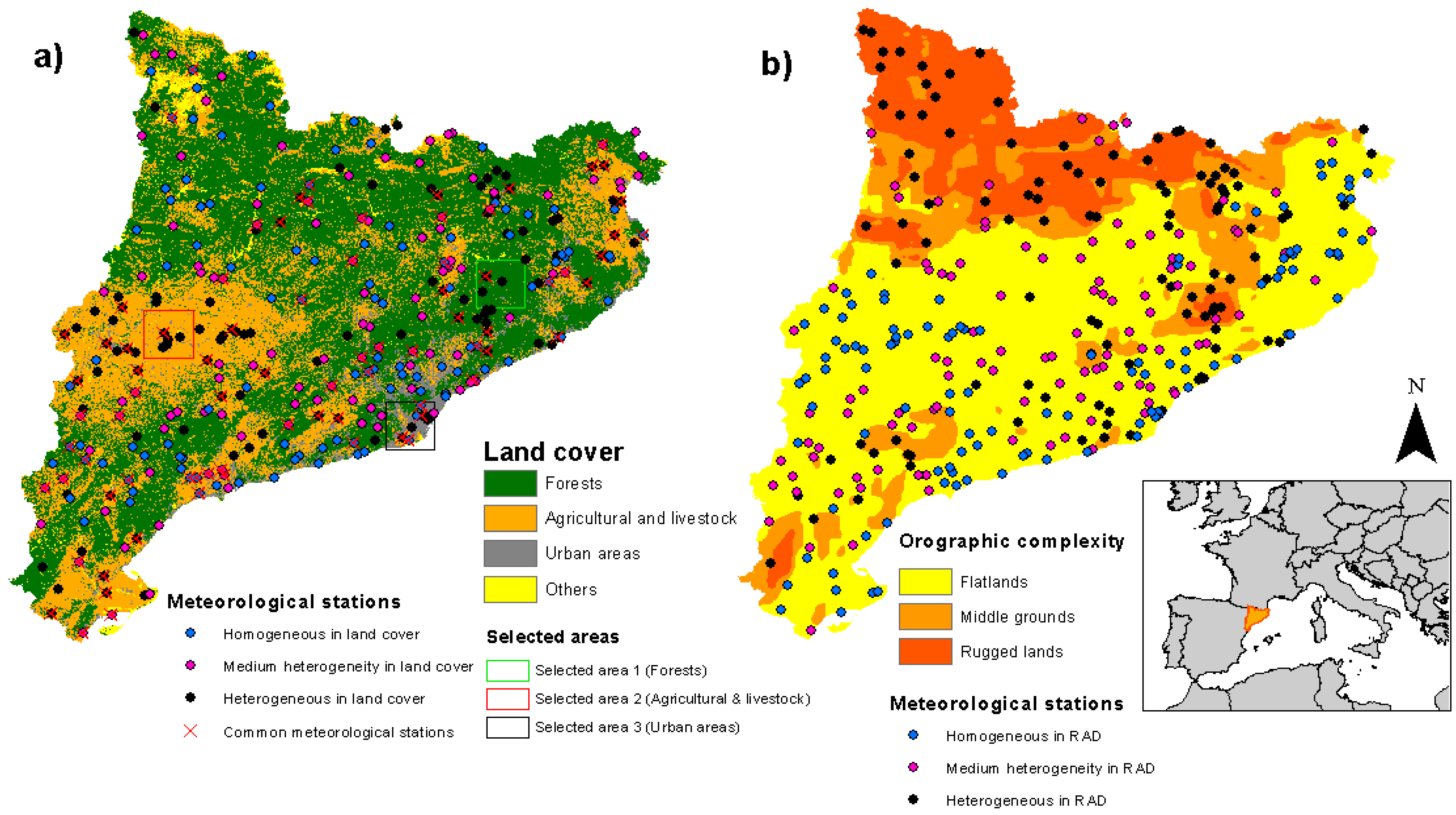
2. Study Area
3. Materials
3.1. Meteorological Station Data
3.2. Other Geographic Data
3.3. Satellite Land Surface Temperature
3.3.1. MODIS Data
3.3.2. ATSR Data
4. Methodology
4.1. Including LST in the Air Temperature Interpolation Scheme
4.2. Segmentation Based on Land Cover and Orographic Complexity
4.3. Analysis of LST Spatial Scale
4.4. Weighted Linear Regression Based on LST Quality Bands
4.5. Performance Metrics
5. Results
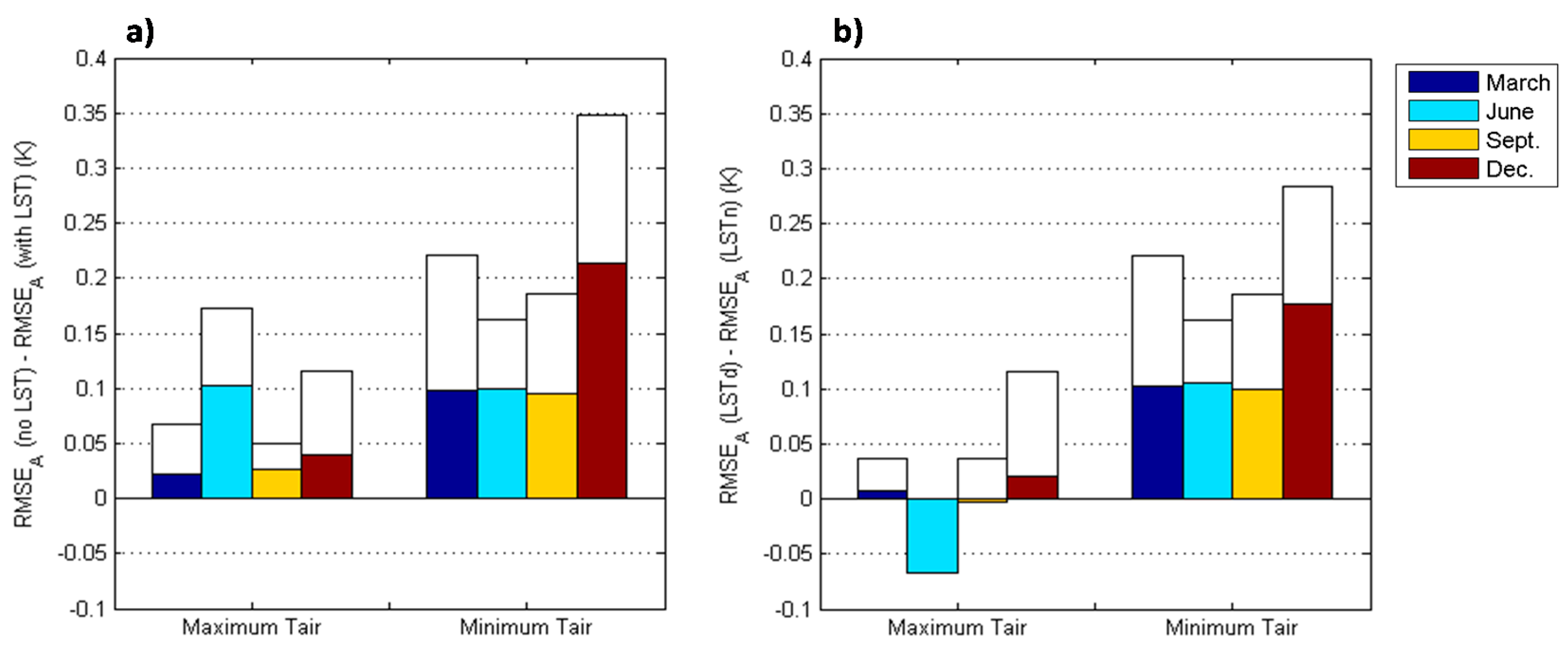
5.1. Effect of Considering the LST Quality
5.2. Effect of LST Spatial Scale
5.2.1. Analysis in Terms of the Heterogeneity in Solar Radiation
5.2.2. Analysis in Terms of the Heterogeneity in Land Cover
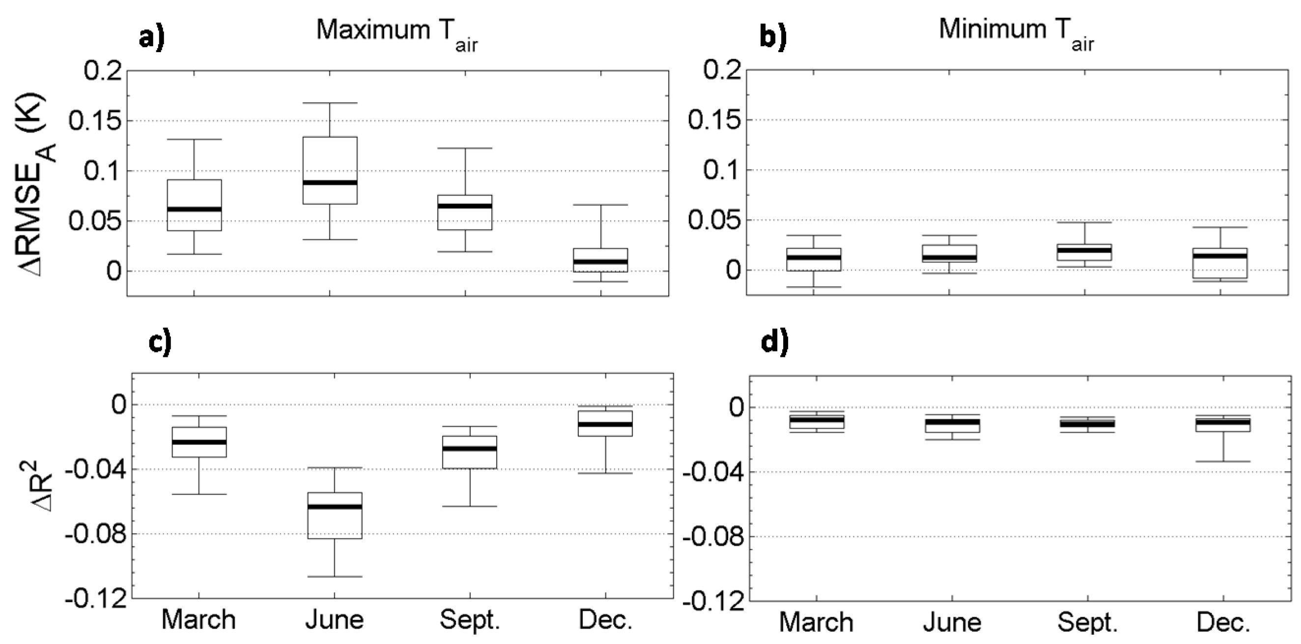
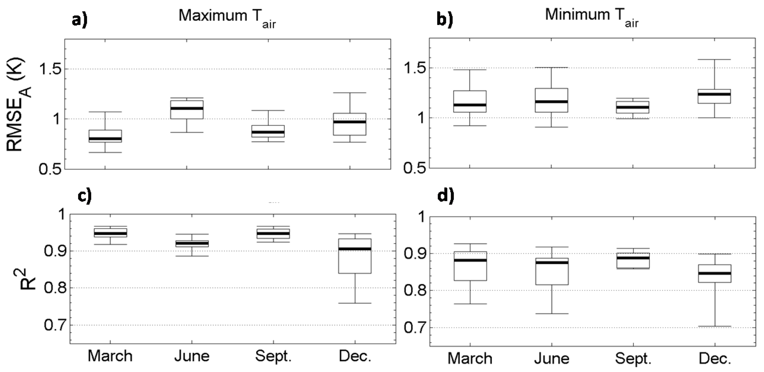
5.3. Statistical Comparisons of Model Performance
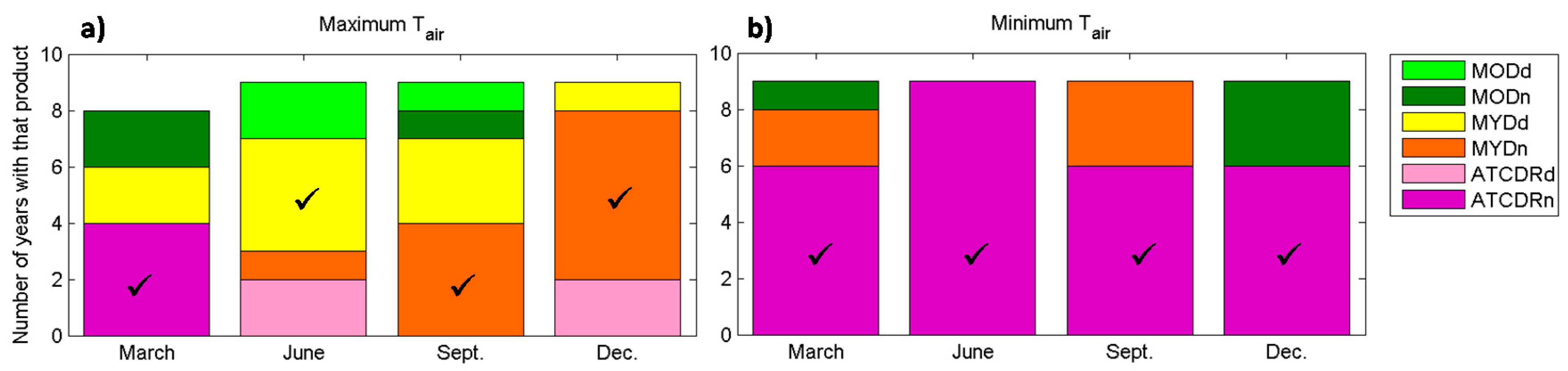
5.3.1. Models with a Set of Common Meteorological Stations
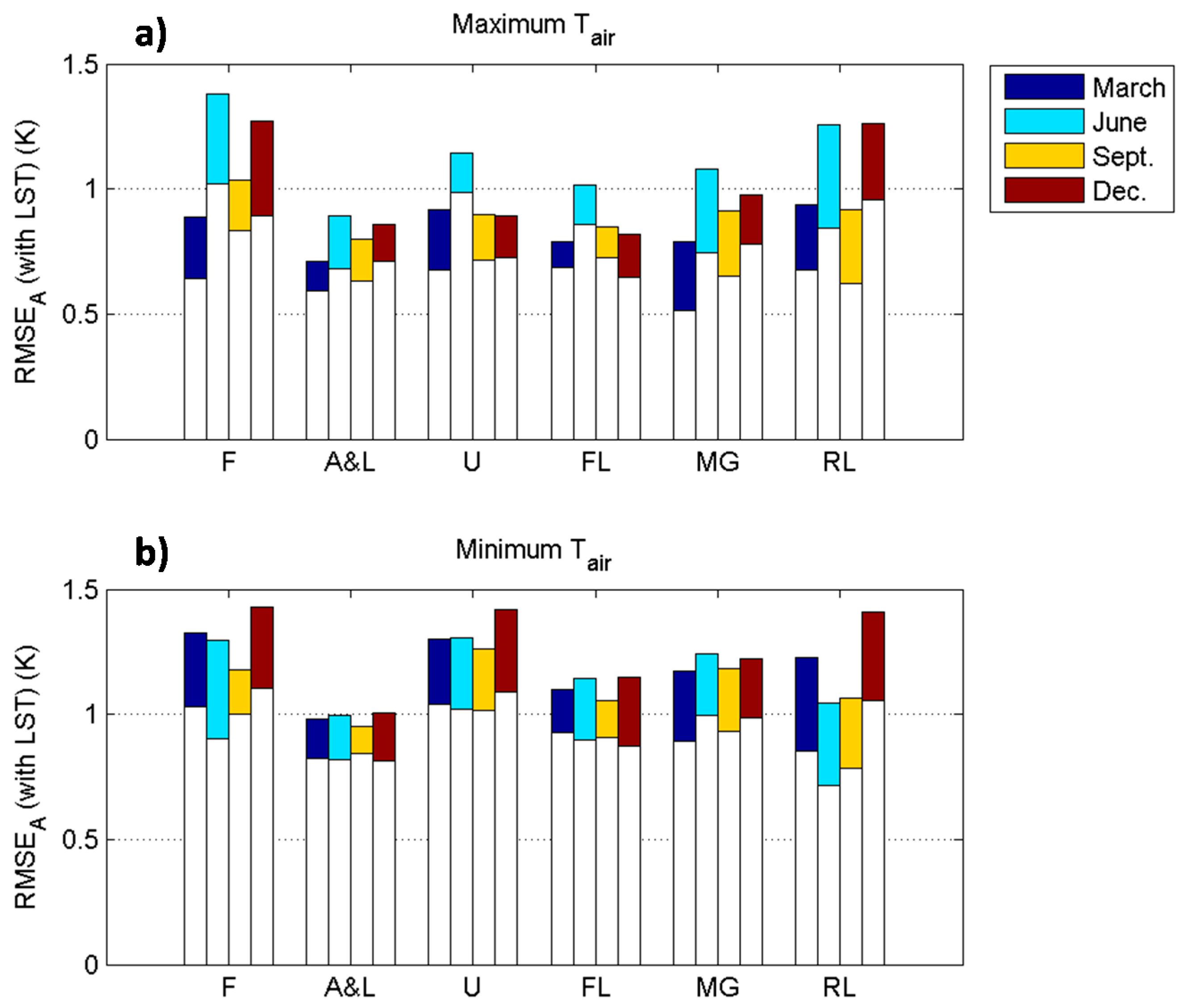
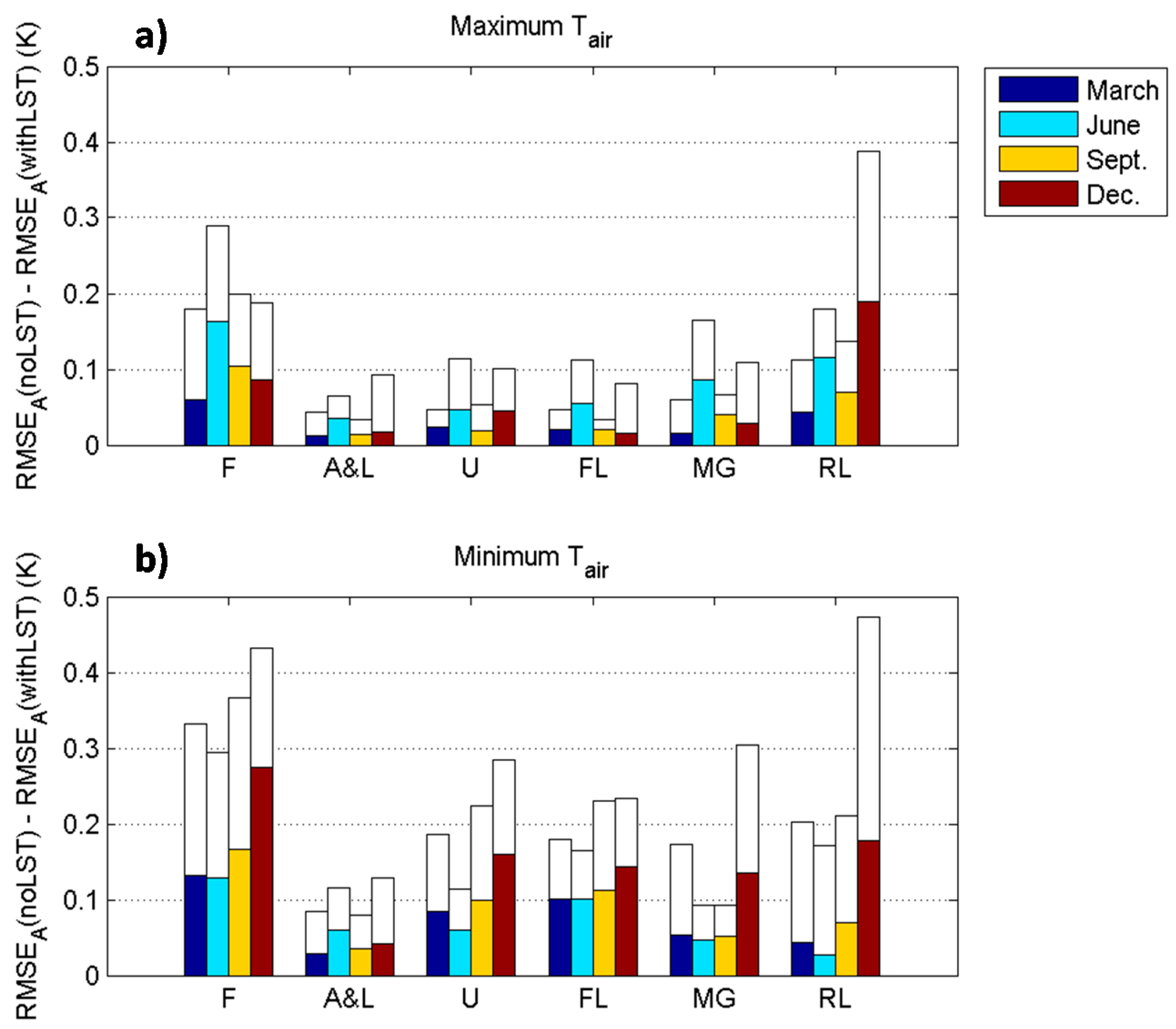
5.3.2. Analysis Segmented by Land Cover and Orographic Complexity
5.3.3. Implication of Model Complexity
5.3.4. Overall Performance
6. Discussion
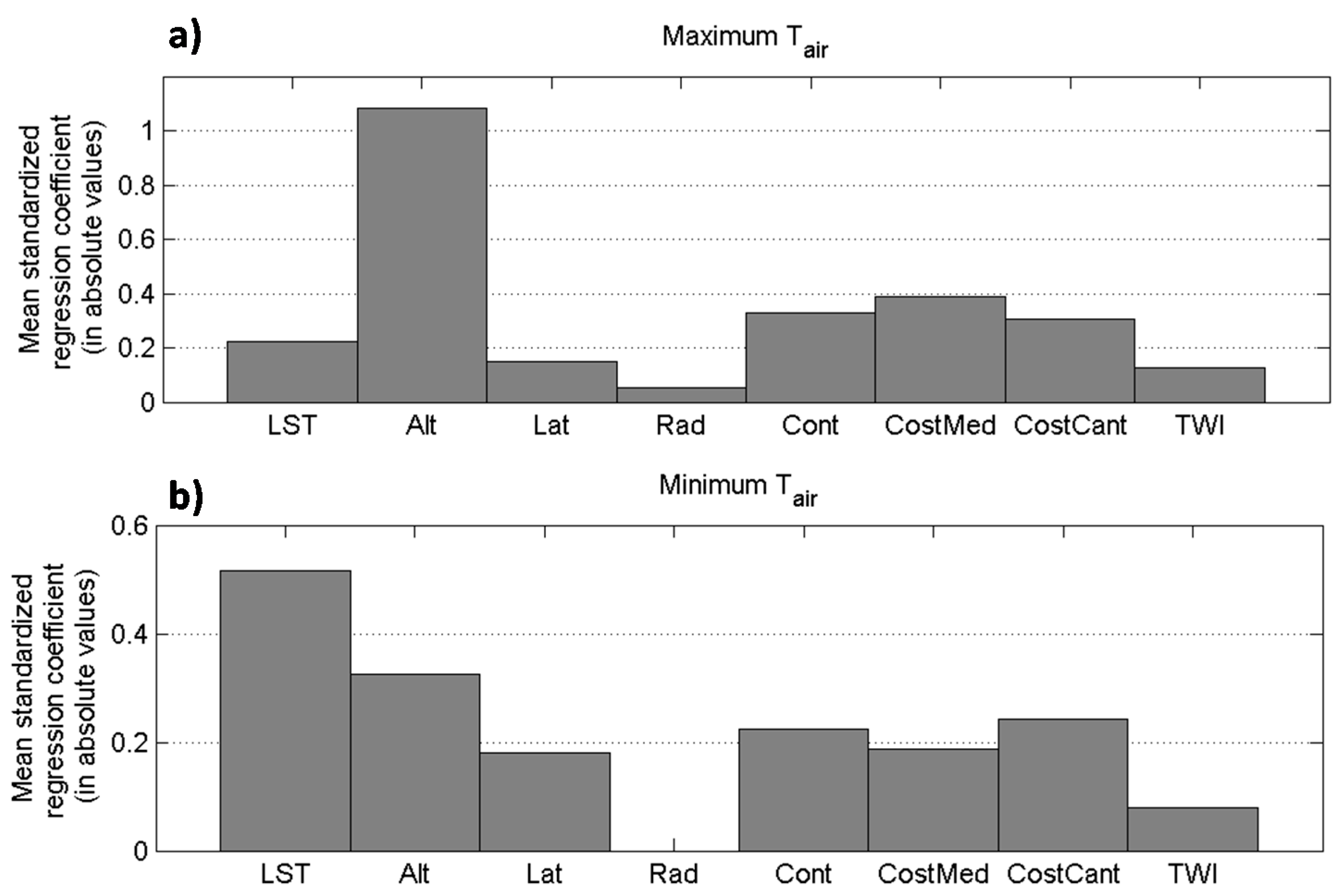
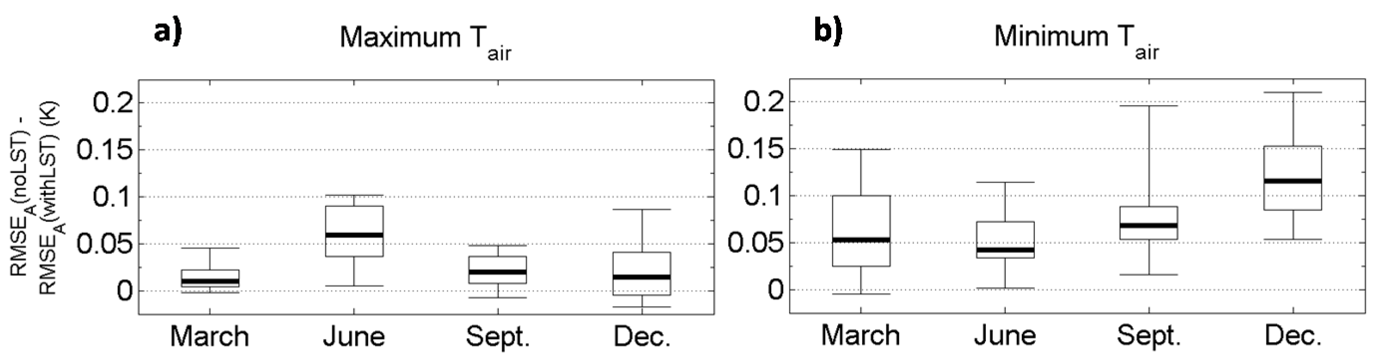
6.1. Improvements from Including LST
6.2. Differences between Daytime and Nighttime LST
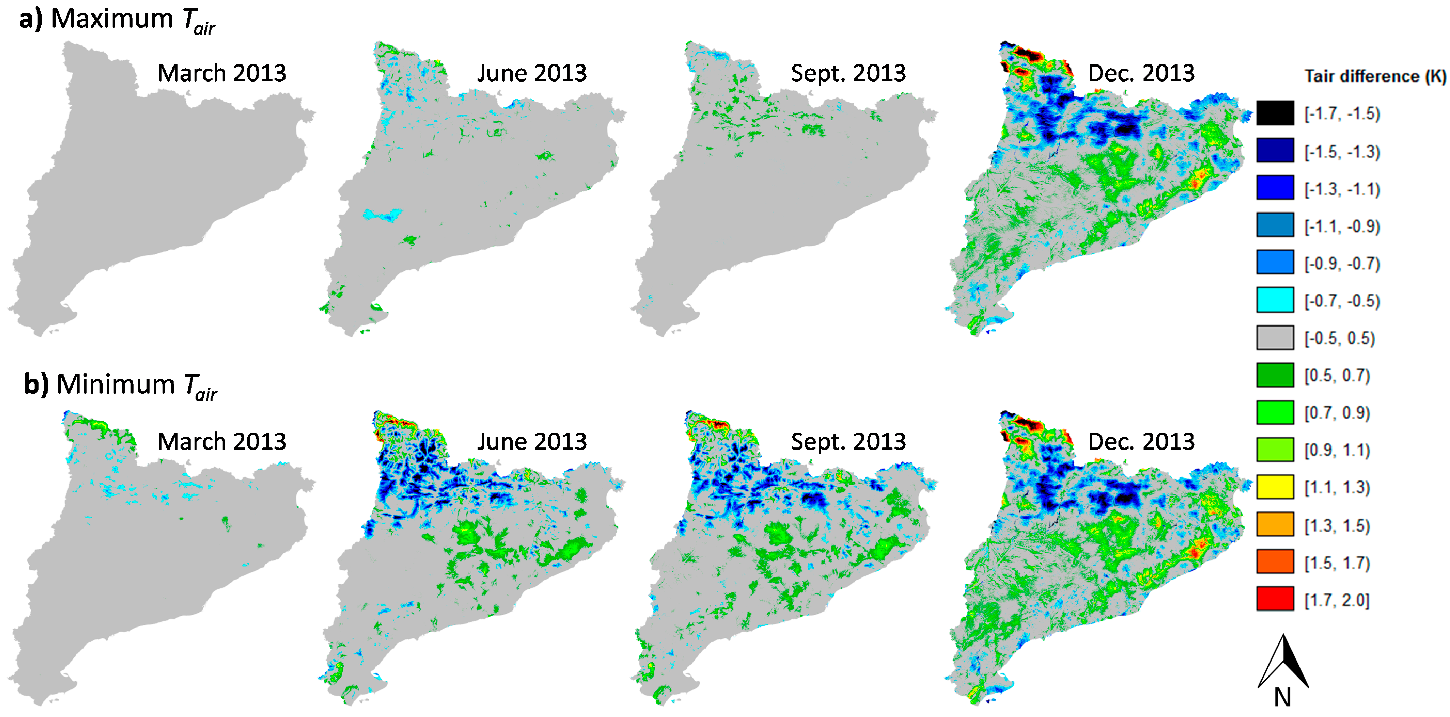
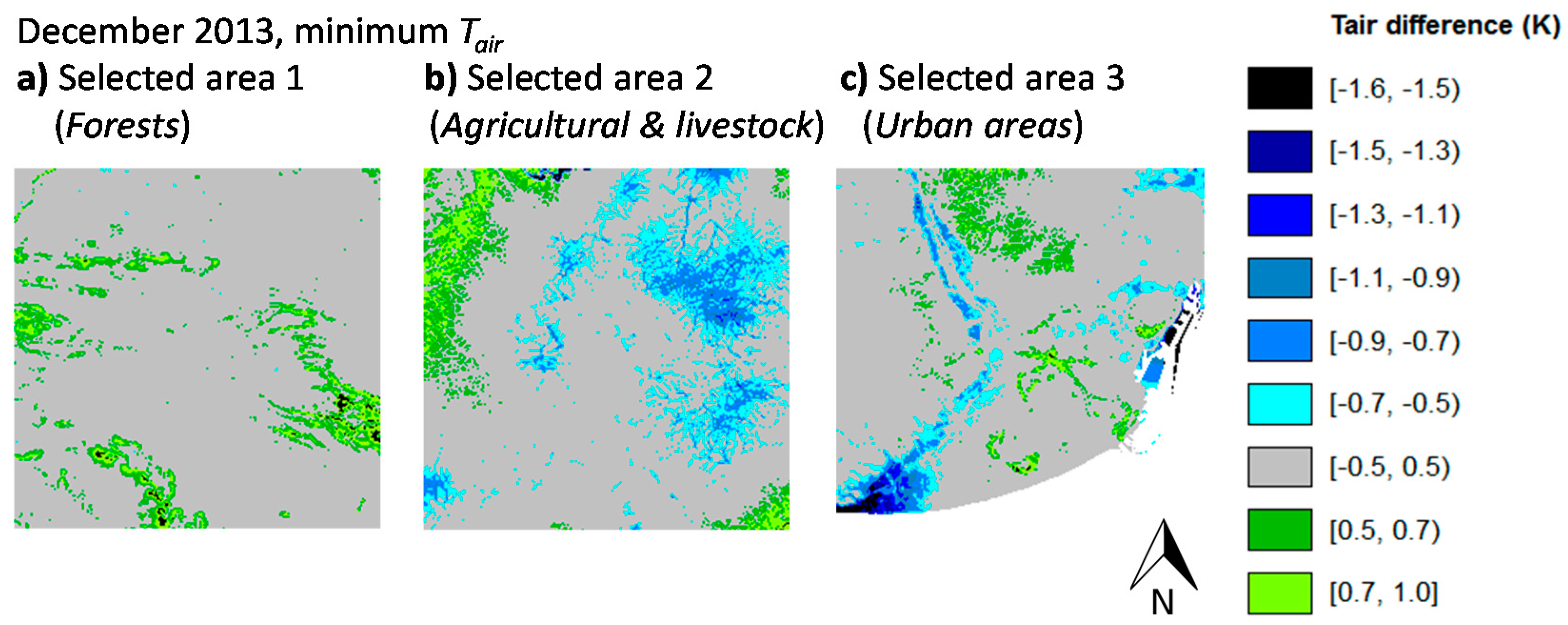
6.3. Temporal and Spatial Patterns
7. Conclusions
Acknowledgments
Author Contributions
Conflicts of Interest
References
- Wylie, R.G.; Lalas, T. Measurement of Temperature and Humidity; Technical Note No. 194, WMO-No. 759; World Meteorological Organization (WMO): Geneva, Switzerland, 1992. [Google Scholar]
- Idso, S.B. A set of equations for full spectrum and 8 µm to 14 µm and 10.5 µm to 12.5 µm thermal radiation from cloudless skies. Water Resour. Res. 1981, 17, 295–304. [Google Scholar] [CrossRef]
- Kustas, W.P.; Norman, J.M. Use of remote sensing for evapotranspiration monitoring over land surfaces. Hydrol. Sci. J. 1996, 41, 495–516. [Google Scholar] [CrossRef]
- Prihodko, L.; Goward, S.N. Estimation of air temperature from remotely sensed surface observations. Remote Sens. Environ. 1997, 60, 335–346. [Google Scholar] [CrossRef]
- Bastiaanssen, W.G.M.; Menenti, M.; Feddes, R.A.; Holtslag, A.A.M. A remote sensing surface energy balance algorithm for land (SEBAL)-1. Formulation. J. Hydrol. 1998, 213, 198–212. [Google Scholar] [CrossRef]
- Kustas, W.P.; French, A.N.; Hatfield, J.L.; Jackson, T.J.; Moran, M.S.; Rango, A.; Ritchie, J.C.; Schmugge, T.J. Remote sensing research in hydrometeorology. Photogramm. Eng. Remote Sens. 2003, 69, 631–646. [Google Scholar] [CrossRef]
- Kuhn, K.G.; Campbell-Lendrum, D.H.; Davies, C.R. A continental risk map for malaria mosquito (Diptera: Culicidae) vectors in Europe. J. Med. Entomol. 2002, 39, 621–630. [Google Scholar] [CrossRef] [PubMed]
- Chow, V.T.; Maidment, D.R.; Mays, L.W. Applied Hydrology; Mcgraw-Hill: Singapore, 1998. [Google Scholar]
- Prince, S.D.; Goward, S.N. Global primary production: A remote sensing approach. J. Biogeogr. 1995, 22, 815–835. [Google Scholar] [CrossRef]
- IPCC. Climate change 2007: The physical science basis. In Contribution of Working Group I to the Fourth Assessment Report of the Intergovernmental Panel on Climate Change; Solomon, S., Qin, D., Manning, M., Chen, Z., Marquis, M., Averyt, K.B., Tignor, M., Miller, H.L., Eds.; Cambridge University Press: Cambridge, UK, 2007. [Google Scholar]
- Vicente-Serrano, S.M.; Heredia-Laclaustra, A. Nao influence on NDVI trends in the Iberian Peninsula (1982–2000). Int. J. Remote Sens. 2004, 25, 2871–2879. [Google Scholar] [CrossRef]
- Sun, Y.J.; Wang, J.F.; Zhang, R.H.; Gillies, R.R.; Xue, Y.; Bo, Y.C. Air temperature retrieval from remote sensing data based on thermodynamics. Theor. Appl. Climatol. 2005, 80, 37–48. [Google Scholar] [CrossRef]
- Cristóbal, J.; Ninyerola, M.; Pons, X. Modeling air temperature through a combination of remote sensing and gis data. J. Geophys. Res. Atmos. 2008, 113. [Google Scholar] [CrossRef]
- Hengl, T.; Heuvelink, G.B.M.; Tadic, M.P.; Pebesma, E.J. Spatio-temporal prediction of daily temperatures using time-series of MODIS LST images. Theor. Appl. Climatol. 2012, 107, 265–277. [Google Scholar] [CrossRef]
- Yang, Y.; Cai, W.; Yang, J. Evaluation of MODIS land surface temperature data to estimate near-surface air temperature in northeast China. Remote Sens. 2017, 9, 410. [Google Scholar] [CrossRef]
- Benali, A.; Carvalho, A.C.; Nunes, J.P.; Carvalhais, N.; Santos, A. Estimating air surface temperature in Portugal using MODIS LST data. Remote Sens. Environ. 2012, 124, 108–121. [Google Scholar] [CrossRef]
- Xu, Y.M.; Knudby, A.; Ho, H.C. Estimating daily maximum air temperature from MODIS in British Columbia, Canada. Int. J. Remote Sens. 2014, 35, 8108–8121. [Google Scholar] [CrossRef]
- Vancutsem, C.; Ceccato, P.; Dinku, T.; Connor, S.J. Evaluation of MODIS land surface temperature data to estimate air temperature in different ecosystems over Africa. Remote Sens. Environ. 2010, 114, 449–465. [Google Scholar] [CrossRef]
- Zeng, L.L.; Wardlow, B.D.; Tadesse, T.; Shan, J.; Hayes, M.J.; Li, D.R.; Xiang, D.X. Estimation of daily air temperature based on MODIS land surface temperature products over the corn belt in the US. Remote Sens. 2015, 7, 951–970. [Google Scholar] [CrossRef]
- Mutiibwa, D.; Strachan, S.; Albright, T. Land surface temperature and surface air temperature in complex terrain. IEEE J. Sel. Top. Appl. Earth Obs. Remote Sens. 2015, 8, 4762–4774. [Google Scholar] [CrossRef]
- Mostovoy, G.V.; King, R.L.; Reddy, K.R.; Kakani, V.G.; Filippova, M.G. Statistical estimation of daily maximum and minimum air temperatures from MODIS LST data over the state of Mississippi. Geosci. Remote Sens. 2006, 43, 78–110. [Google Scholar] [CrossRef]
- Zhu, W.B.; Lu, A.F.; Jia, S.F. Estimation of daily maximum and minimum air temperature using MODIS land surface temperature products. Remote Sens. Environ. 2013, 130, 62–73. [Google Scholar] [CrossRef]
- Niclòs, R.; Valiente, J.A.; Barberà, M.J.; Caselles, V. Land surface air temperature retrieval from EOS-MODIS images. IEEE Geosci. Remote Sens. Lett. 2014, 11, 1380–1384. [Google Scholar] [CrossRef]
- Mira, M.; Olioso, A.; Gallego-Elvira, B.; Courault, D.; Garrigues, S.; Marloie, O.; Hagolle, O.; Guillevic, P.; Boulet, G. Uncertainty assessment of surface net radiation derived from Landsat images. Remote Sens. Environ. 2016, 175, 251–270. [Google Scholar] [CrossRef]
- Vazquez, D.P.; Reyes, F.J.O.; Arboledas, L.A. A comparative study of algorithms for estimating land surface temperature from AVHRR data. Remote Sens. Environ. 1997, 62, 215–222. [Google Scholar] [CrossRef]
- Zaksek, K.; Schroedter-Homscheidt, M. Parameterization of air temperature in high temporal and spatial resolution from a combination of the SEVIRI and MODIS instruments. ISPRS J. Photogramm. Remote Sens. 2009, 64, 414–421. [Google Scholar] [CrossRef]
- Vogt, J.V.; Viau, A.A.; Paquet, F. Mapping regional air temperature fields using satellite-derived surface skin temperatures. Int. J. Climatol. 1997, 17, 1559–1579. [Google Scholar] [CrossRef]
- Cresswell, M.P.; Morse, A.P.; Thomson, M.C.; Connor, S.J. Estimating surface air temperatures, from Meteosat land surface temperatures, using an empirical solar zenith angle model. Int. J. Remote Sens. 1999, 20, 1125–1132. [Google Scholar] [CrossRef]
- Jang, J.D.; Viau, A.A.; Anctil, F. Neural network estimation of air temperatures from AVHRR data. Int. J. Remote Sens. 2004, 25, 4541–4554. [Google Scholar] [CrossRef]
- Czajkowski, K.P.; Goward, S.N.; Stadler, S.J.; Walz, A. Thermal remote sensing of near surface environmental variables: Application over the Oklahoma Mesonet. Profr. Geogr. 2000, 52, 345–357. [Google Scholar] [CrossRef]
- Meteotest. Meteonorm Handbook Part II: Theory. 2010. Available online: www.meteonorm.com/images/uploads/downloads/mn72_theory7.2.pdf (accessed on 19 September 2017).
- Ninyerola, M.; Pons, X.; Roure, J.M. A methodological approach of climatological modelling of air temperature and precipitation through GIS techniques. Int. J. Climatol. 2000, 20, 1823–1841. [Google Scholar] [CrossRef]
- Ninyerola, M.; Pons, X.; Roure, J.M. Objective air temperature mapping for the Iberian Peninsula using spatial interpolation and GIS. Int. J. Climatol. 2007, 27, 1231–1242. [Google Scholar] [CrossRef]
- Ninyerola, M.; Pons, X.; Roure, J.M. Monthly precipitation mapping of the Iberian Peninsula using spatial interpolation tools implemented in a geographic information system. Theor. Appl. Climatol. 2007, 89, 195–209. [Google Scholar] [CrossRef] [Green Version]
- Stisen, S.; Sandholt, I.; Norgaard, A.; Fensholt, R.; Eklundh, L. Estimation of diurnal air temperature using MSG Seviri data in West Africa. Remote Sens. Environ. 2007, 110, 262–274. [Google Scholar] [CrossRef]
- Meyer, H.; Katurji, M.; Appelhans, T.; Muller, M.U.; Nauss, T.; Roudier, P.; Zawar-Reza, P. Mapping daily air temperature for Antarctica based on MODIS LST. Remote Sens. 2016, 8, 732. [Google Scholar] [CrossRef]
- Noi, P.; Kappas, M.; Degener, J. Estimating daily maximum and minimum land air surface temperature using MODIS land surface temperature data and ground truth data in northern Vietnam. Remote Sens. 2016, 8, 1002. [Google Scholar] [CrossRef]
- Cai, Y.; Chen, G.; Wang, Y.; Yang, L. Impacts of land cover and seasonal variation on maximum air temperature estimation using MODIS imagery. Remote Sens. 2017, 9, 233. [Google Scholar] [CrossRef]
- Huang, R.; Zhang, C.; Huang, J.; Zhu, D.; Wang, L.; Liu, J. Mapping of daily mean air temperature in agricultural regions using daytime and nighttime land surface temperatures derived fromTerra and Aqua MODIS data. Remote Sens. 2015, 7, 8728–8756. [Google Scholar] [CrossRef]
- Chen, F.G.; Liu, Y.; Liu, Q.; Qin, F. A statistical method based on remote sensing for the estimation of air temperature in China. Int. J. Climatol. 2015, 35, 2131–2143. [Google Scholar] [CrossRef]
- Sahin, M. Modelling of air temperature using remote sensing and artificial neural network in Turkey. Adv. Space Res. 2012, 50, 973–985. [Google Scholar] [CrossRef]
- Yao, Y.H.; Zhang, B.P. MODIS-based air temperature estimation in the southeastern Tibetan Plateau and neighboring areas. J. Geogr. Sci. 2012, 22, 152–166. [Google Scholar] [CrossRef]
- Shen, L.; Guo, X.L.; Xiao, K. Spatiotemporally characterizing urban temperatures based on remote sensing and GIS analysis: A case study in the city of Saskatoon (SK, Canada). Open Geosci. 2015, 7, 27–39. [Google Scholar] [CrossRef]
- Clavero, P.; Martín-Vide, J.; Raso-Nadal, J. Atles Climàtic de Catalunya. Termopluviometria i Radiació Solar; Servei Meteorològic de Catalunya, Generalitat de Catalunya (Departament de Política Territorrial i Obres Públiques), Institut Cartogràfic de Catalunya and Departament de Medi Ambient: Barcelona, Spain, 1996. [Google Scholar]
- Folch i Guillèn, R. La Vegetació dels Països Catalans, 2nd ed.; Institució Catalana D’història Natural, Memoria Núm. 10; Editorial Ketres: Barcelona, Spain, 1986. [Google Scholar]
- Ibáñez, J.; Burriel, J. Mcsc: A High-Resolution Thematic Digital Cartography. In Proceedings of the 5th European Congress on Regional Geoscientific Cartography and Information Systems, Barcelona, Spain, 13–16 June 2006; pp. 278–280. [Google Scholar]
- Spanish National Meteorological Agency (Aemet). Available online: http://www.aemet.es (accessed on 19 September 2017).
- Catalan Meteorological Service (SMC). Available online: http://www.meteo.cat (accessed on 19 September 2017).
- Pons, X. Estimación de la radiación solar a partir de modelos digitales de elevaciones. Propuesta metodológica. In VII Coloquio de Geografía Cuantitativa, Sistemas de Información Geográfica y Teledetección; Juaristi, J., Moro, I., Eds.; Association of Spanish Geographers: Vitoria-Gasteiz, Spain, 1996; pp. 87–97. [Google Scholar]
- Pons, X.; Ninyerola, M. Mapping a topographic global solar radiation model implemented in a GIS and refined with ground data. Int. J. Climatol. 2008, 28, 1821–1834. [Google Scholar] [CrossRef]
- Böhner, J.; Köthe, R.; Conrad, O.; Gross, J.; Ringeler, A.; Selige, T. Soil regionalisation by means of terrain analysis and process parameterisation. In Soil Classification 2001; Micheli, E., Nachtergaele, F., Montanarella, L., Eds.; European Soil Bureau, Research Report No. 7, EUR 20398 EN; European Commission: Luxembourg, 2002; pp. 213–222. [Google Scholar]
- Pypker, T.G.; Barnard, H.R.; Hauck, M.; Sulzman, E.W.; Unsworth, M.H.; Mix, A.C.; Kennedy, A.M.; Bond, B.J. Can carbon isotopes be used to predict watershed-scale transpiration? Water Resour. Res. 2009, 45. [Google Scholar] [CrossRef]
- Prabhakara, C.; Dalu, G.; Kunde, V.G. Estimation of sea surface temperature from remote sensing in 11 to 13 µm window region. J. Geophys. Res. 1974, 79, 5039–5044. [Google Scholar] [CrossRef]
- Deschamps, P.Y.; Phulpin, T. Atmospheric correction of infrared measurements of sea surface temperature using channels at 3.7, 11 and 12 µm. Bound. Layer Meteorol. 1980, 18, 131–143. [Google Scholar] [CrossRef]
- Becker, F.; Li, Z.L. Towards a local split window method over land surfaces. Int. J. Remote Sens. 1990, 11, 369–393. [Google Scholar] [CrossRef]
- Wan, Z.M.; Dozier, J. A generalized split-window algorithm for retrieving land-surface temperature from space. IEEE Trans. Geosci. Remote Sens. 1996, 34, 892–905. [Google Scholar]
- Coll, C.; Caselles, V. A split-window algorithm for land surface temperature from advanced very high resolution radiometer data: Validation and algorithm comparison. J. Geophys. Res. Atmos. 1997, 102, 16697–16713. [Google Scholar] [CrossRef]
- Wan, Z.M.; Zhang, Y.L.; Zhang, Q.C.; Li, Z.L. Validation of the land-surface temperature products retrieved from Terra moderate resolution imaging spectroradiometer data. Remote Sens. Environ. 2002, 83, 163–180. [Google Scholar] [CrossRef]
- Wan, Z.M. MODIS Land-Surface Temperature. Algorithm Theoretical Basis Document. 1999. Available online: http://modis.gsfc.nasa.gov/data/atbd/atbd_mod11.pdf (accessed on 19 September 2017).
- Snyder, W.C.; Wan, Z.; Zhang, Y.; Feng, Y.Z. Classification-based emissivity for land surface temperature measurement from space. Int. J. Remote Sens. 1998, 19, 2753–2774. [Google Scholar] [CrossRef]
- Wan, Z.M. Collection-6 MODIS Land Surface Temperature Products. Users’ Guide; Eri, University of California: Santa Barbara, CA, USA, 2013. [Google Scholar]
- Wan, Z.; Zhang, Y.; Zhang, Q.; Li, Z.L. Quality assessment and validation of the MODIS global land surface temperature. Int. J. Remote Sens. 2004, 25, 261–274. [Google Scholar] [CrossRef]
- Wan, Z.M. New refinements and validation of the MODIS land-surface temperature/emissivity products. Remote Sens. Environ. 2008, 112, 59–74. [Google Scholar] [CrossRef]
- Wan, Z. New refinements and validation of the collection-6 MODIS land-surface temperature/emissivity product. Remote Sens. Environ. 2014, 140, 36–45. [Google Scholar] [CrossRef]
- Wan, Z.M. Mod11b3 MODIS/Terra Land Surface Temperature/Emissivity Monthly l3 Global 6km Sin Grid v006. NASA EOSDIS Land Processes DAAC. 2015. Available online: https://doi.Org/10.5067/modis/mod11b3.006 (accessed on 19 September 2017).
- Prata, A. Land Surface Temperature Measurement from Space: AATSR Algorithm Theoretical Basis Document; Technical Report; CSIRO: Canberra, Australia, 2000; 27p. [Google Scholar]
- Globtemperature Data Portal. Available online: http://data.globtemperature.info (accessed on 19 September 2017).
- Ghent, D. Land Surface Temperature Validation and Algorithm Verification; Report to European Space Agency (UL-NILU-ESA-LST-VAV); European Space Agency: Paris, France, 2012. [Google Scholar]
- Ghent, D.; Corlett, G.; Remedios, J. Advancing the AATSR land surface temperature retrieval with higher resolution auxiliary datasets: Part B—Validation. 2017. in preparation. [Google Scholar]
- Ninyerola, M.; Pons, X.; Roure, J.M. Atlas Climático Digital de la Península Ibérica. Metodología y Aplicaciones en Bioclimatología y Geobotánica; Universitat Autònoma de Barcelona: Bellaterra, Spain, 2005; 44p, Available online: http://opengis.uab.es/wms/iberia/pdf/acdpi.pdf (accessed on 19 September 2017).
- Land Cover Map of Catalonia. CREAF–Generalitat de Catalunya. Available online: http://www.creaf.uab.cat/mcsc/usa/index.htm (accessed on 19 September 2017).
- Atlas Climático Digital de Catalunya. UAB. Available online: http://www.opengis.uab.cat/acdc/espanol/es_presentacio.htm (accessed on 19 September 2017).


| Data | Source or Product Name | Dates | Density/Resolution | |
|---|---|---|---|---|
| Meteorological station data | AEMET (www.aemet.es) SMC (www.meteo.cat) | 2003–2015 | 179–329 stations for each month | |
| Other geographic data | Digital Elevation Model | Cartographic Institute of Catalonia (www.icgc.cat) | 2004–2007 | 15 m |
| Satellite LST | MODIS | MOD11B3 and MYD11B3 | 2003–2015 | 5568 m |
| AATSR and ATSR-2 | ATSR LST Climate Data Record Level-3 | 2003–2011 | 0.05° | |
| Product | Daytime | Nighttime |
|---|---|---|
| MOD11B3 | 10:12–12:00 (11:11) | 21:20–23:00 (21:59) |
| MYD11B3 | 12:24–13:36 (13:08) | 01:24–02:36 (2:04) |
| ATCDR | 10:11–10:59 (10:26) | 21:08–22:01 (21:24) |
| QC-LST | QC-Emis | Weighting (%) |
|---|---|---|
| 1 | 1,2,3,4 | 100 |
| 3 | 1 | 70 |
| 3 | 2 | 50 |
| 3 | 3 | 30 |
| 3 | 4 | 10 |
| ATCDR | |
|---|---|
| δLST (K) | Weighting (%) |
| ≤1 | 100 |
| >1 to ≤1.2 | 90 |
| >1.2 to ≤1.4 | 80 |
| >1.4 to ≤1.6 | 70 |
| >1.6 to ≤1.8 | 60 |
| >1.8 to ≤2.0 | 50 |
| >2.0 to ≤2.3 | 40 |
| >2.3 to ≤2.6 | 30 |
| >2.6 to ≤3.0 | 20 |
| >3.0 | 10 |
| N | LST | Rad | RMSEA (K) | R2 | ||||
|---|---|---|---|---|---|---|---|---|
| noLST | withLST | noLST | withLST | noLST | withLST | |||
| Homo. in Rad | 109 | 0.28 | × | × | 0.80 | 0.77 | 0.55 | 0.61 |
| Hetero. in Rad | 109 | 0.08 | 0.069 | 0.074 | 0.78 | 0.78 | 0.97 | 0.97 |
| Homo. in land cover | 109 | 0.17 | 0.037 | 0.035 | 1.00 | 0.97 | 0.94 | 0.95 |
| Hetero. in land cover | 109 | × | 0.106 | 0.106 | 1.08 | 1.08 | 0.91 | 0.91 |
| All meteo. stations | 327 | 0.10 | 0.066 | 0.063 | 0.80 | 0.79 | 0.93 | 0.94 |
© 2017 by the authors. Licensee MDPI, Basel, Switzerland. This article is an open access article distributed under the terms and conditions of the Creative Commons Attribution (CC BY) license (http://creativecommons.org/licenses/by/4.0/).
Share and Cite
Mira, M.; Ninyerola, M.; Batalla, M.; Pesquer, L.; Pons, X. Improving Mean Minimum and Maximum Month-to-Month Air Temperature Surfaces Using Satellite-Derived Land Surface Temperature. Remote Sens. 2017, 9, 1313. https://doi.org/10.3390/rs9121313
Mira M, Ninyerola M, Batalla M, Pesquer L, Pons X. Improving Mean Minimum and Maximum Month-to-Month Air Temperature Surfaces Using Satellite-Derived Land Surface Temperature. Remote Sensing. 2017; 9(12):1313. https://doi.org/10.3390/rs9121313
Chicago/Turabian StyleMira, Maria, Miquel Ninyerola, Meritxell Batalla, Lluís Pesquer, and Xavier Pons. 2017. "Improving Mean Minimum and Maximum Month-to-Month Air Temperature Surfaces Using Satellite-Derived Land Surface Temperature" Remote Sensing 9, no. 12: 1313. https://doi.org/10.3390/rs9121313