Comparison of Spatial Interpolation and Regression Analysis Models for an Estimation of Monthly Near Surface Air Temperature in China

 ,
, 

Abstract
:
1. Introduction
2. Study Area and Materials
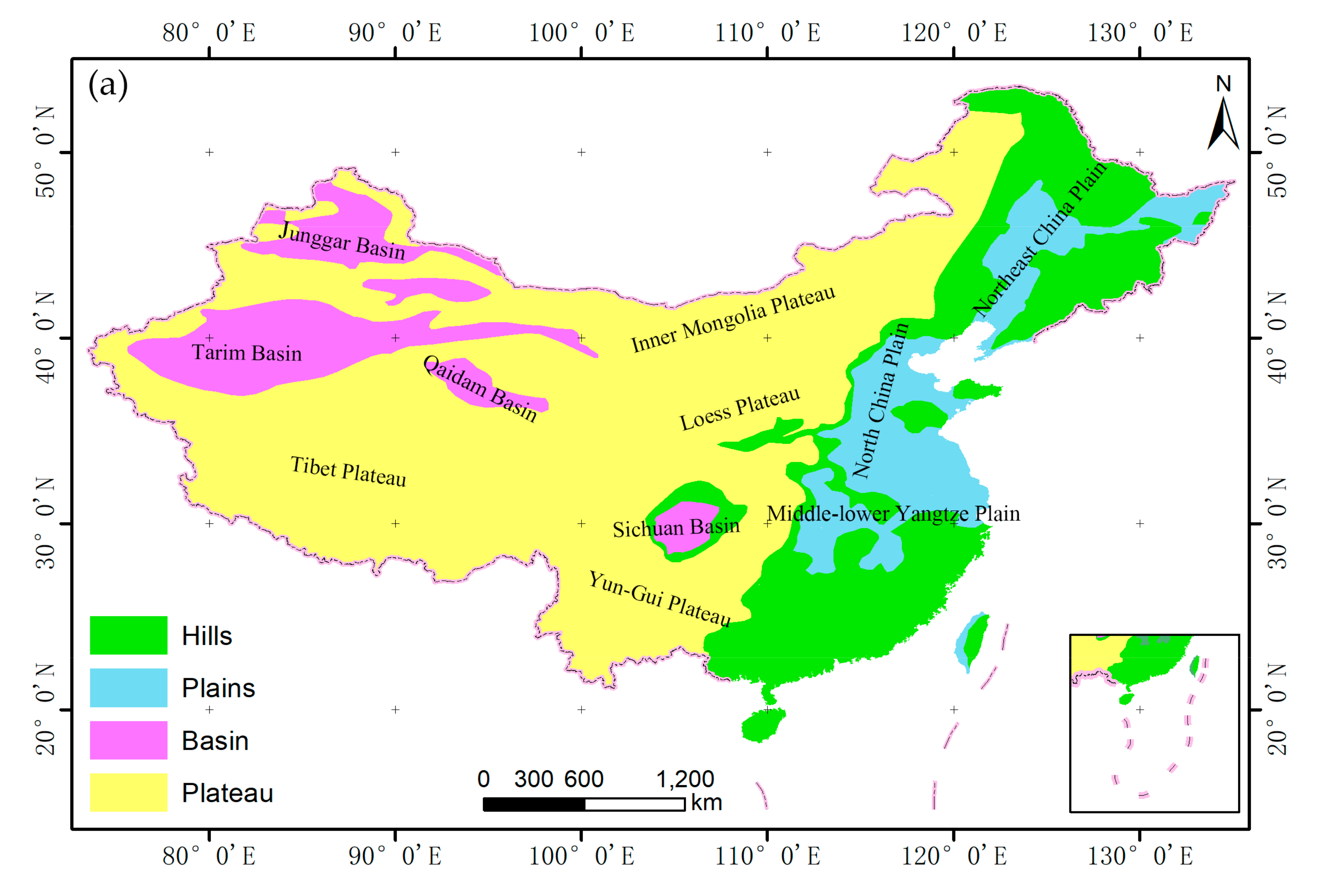
2.1. Study Area
2.2. Satellite Data
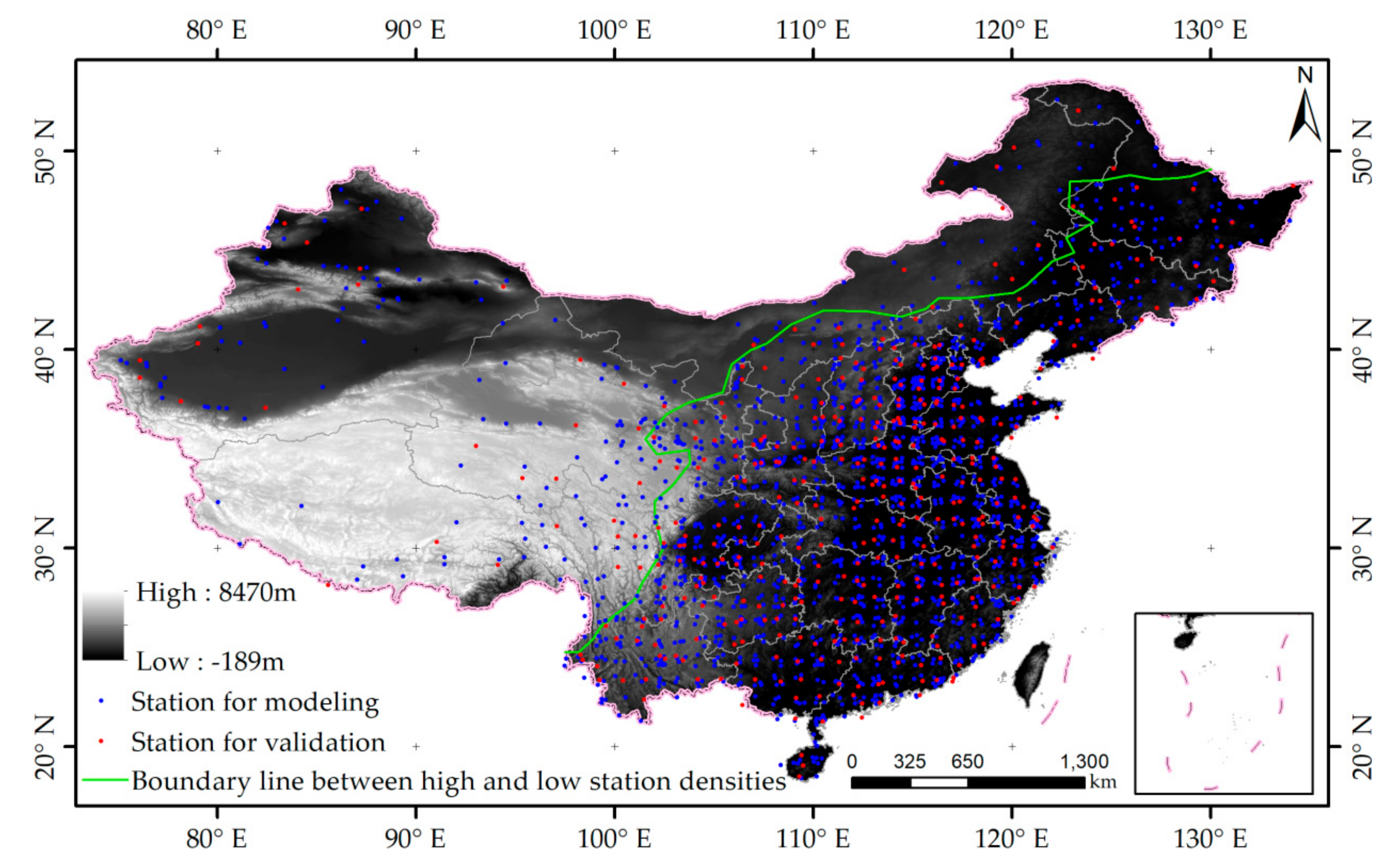
2.3. Station Data
2.4. Elevation Data
3. Methods
3.1. Spatial Interpolation Models
3.2. Standard Multiple Linear Regression Model
3.3. Geographically Weighted Regression Model
3.4. Validation
4. Results
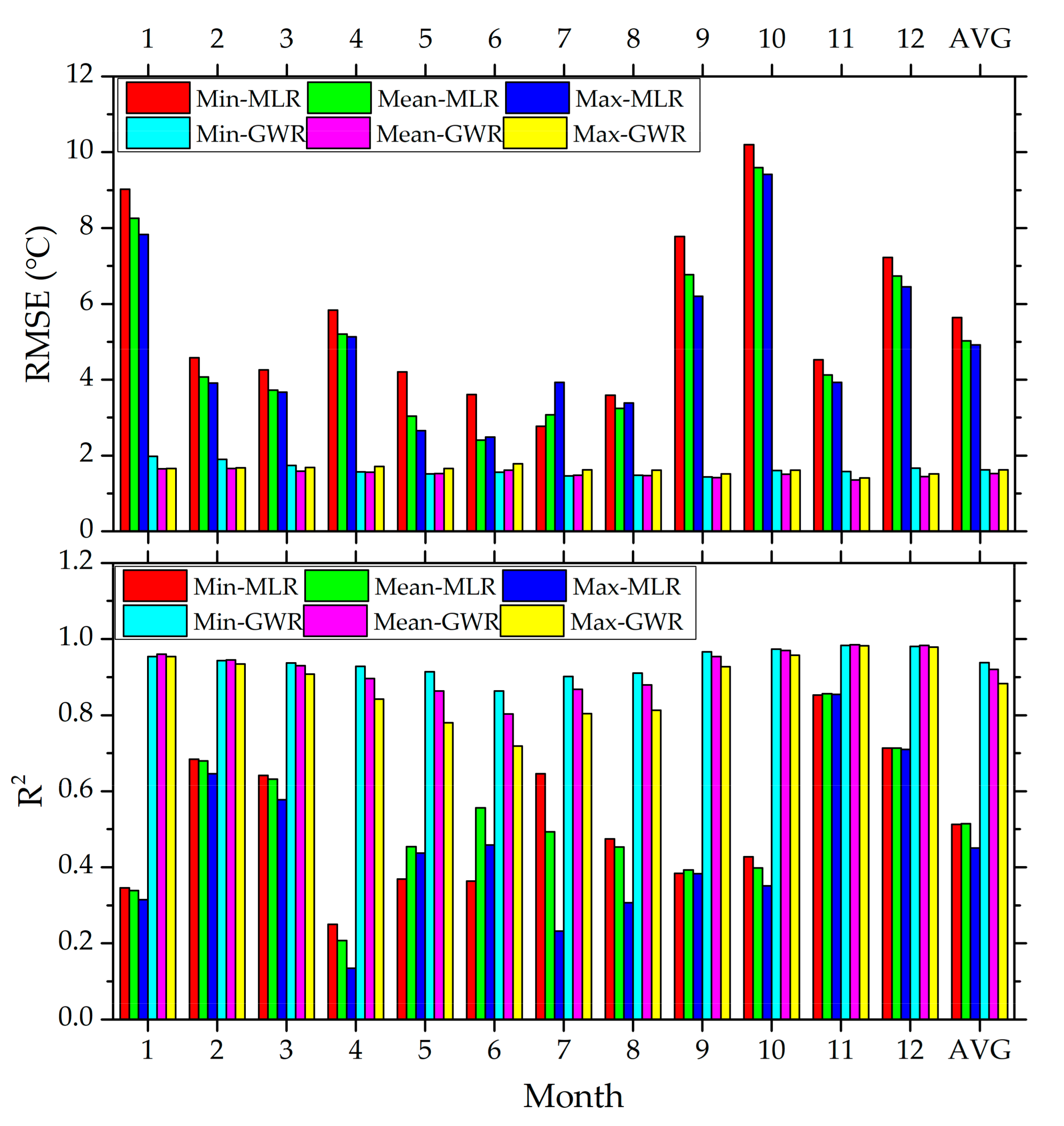
4.1. Comparison between Multiple Linear Regression and Geographically Weighted Regression Models
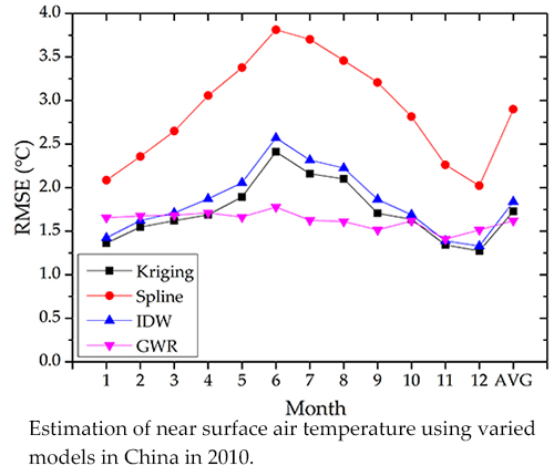
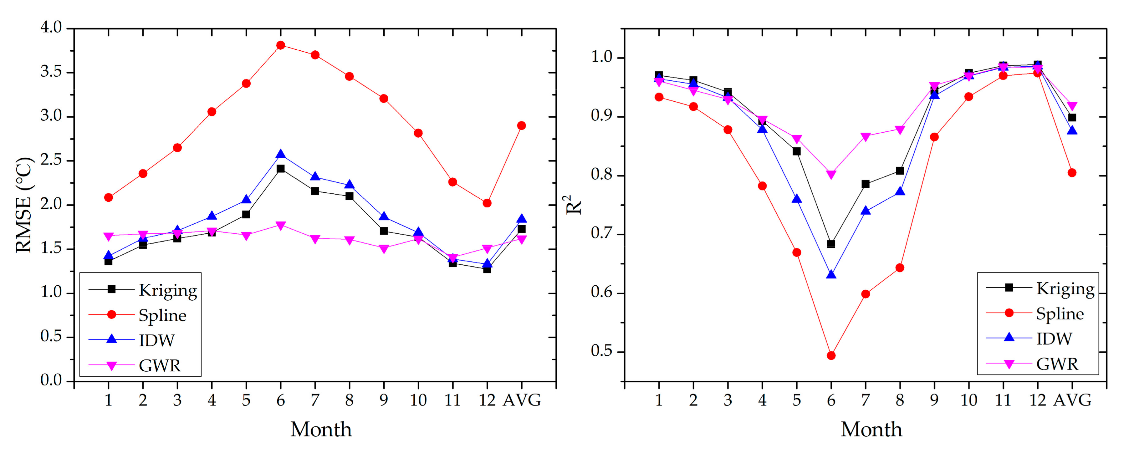
4.2. Comparison between Geographically Weighted Regression and Various Interpolation Models
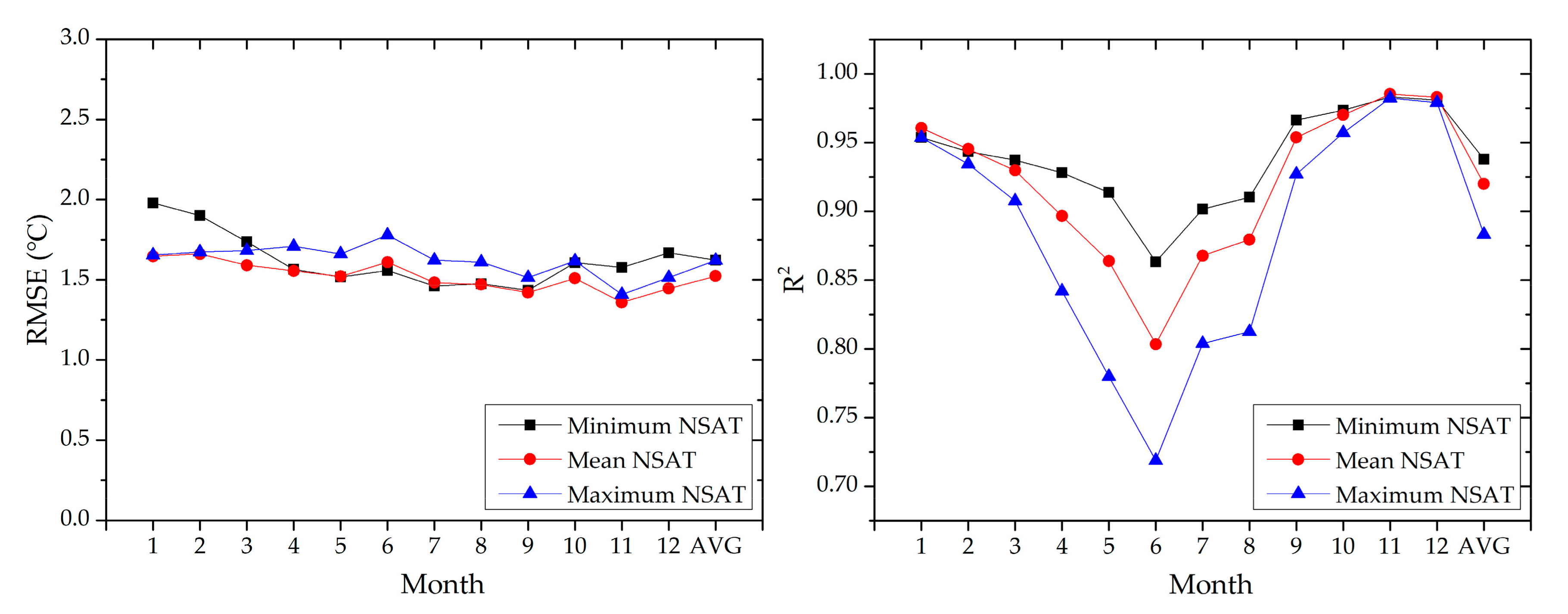
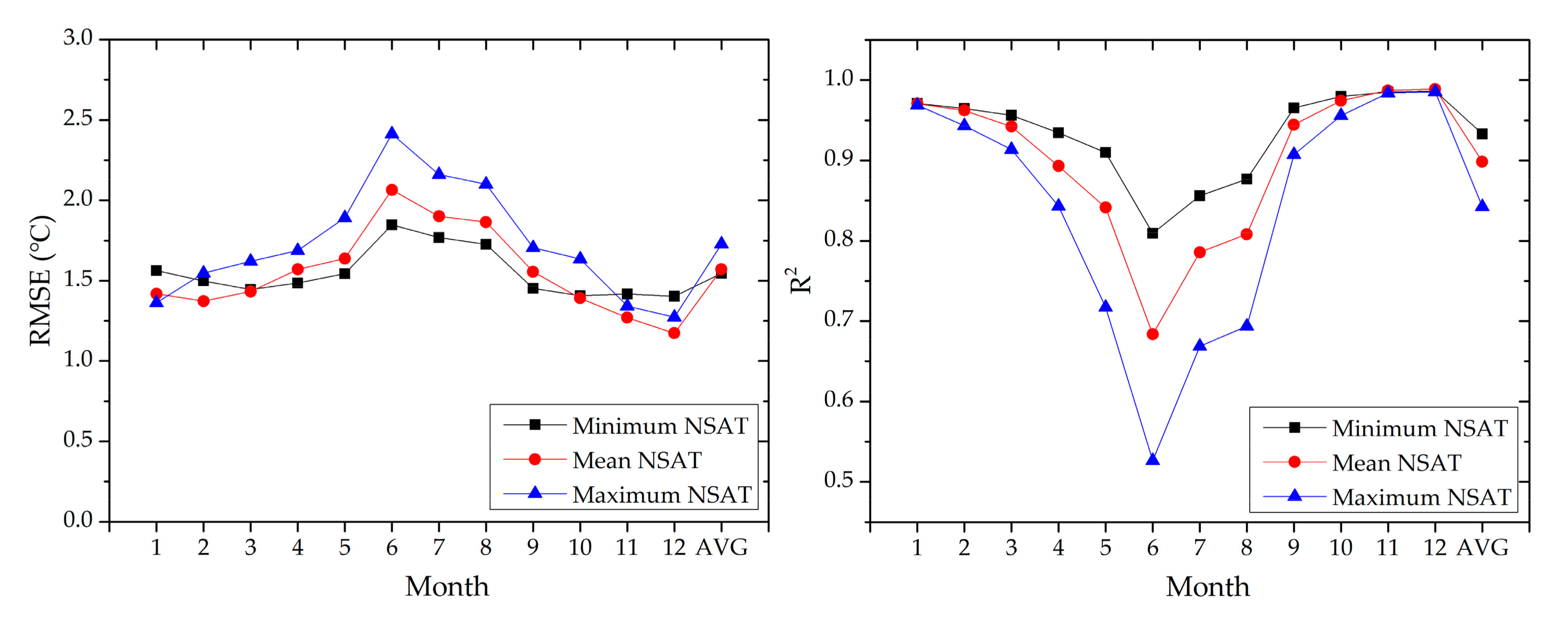
4.3. Comparison between Different Near Surface Air Temperature Variables
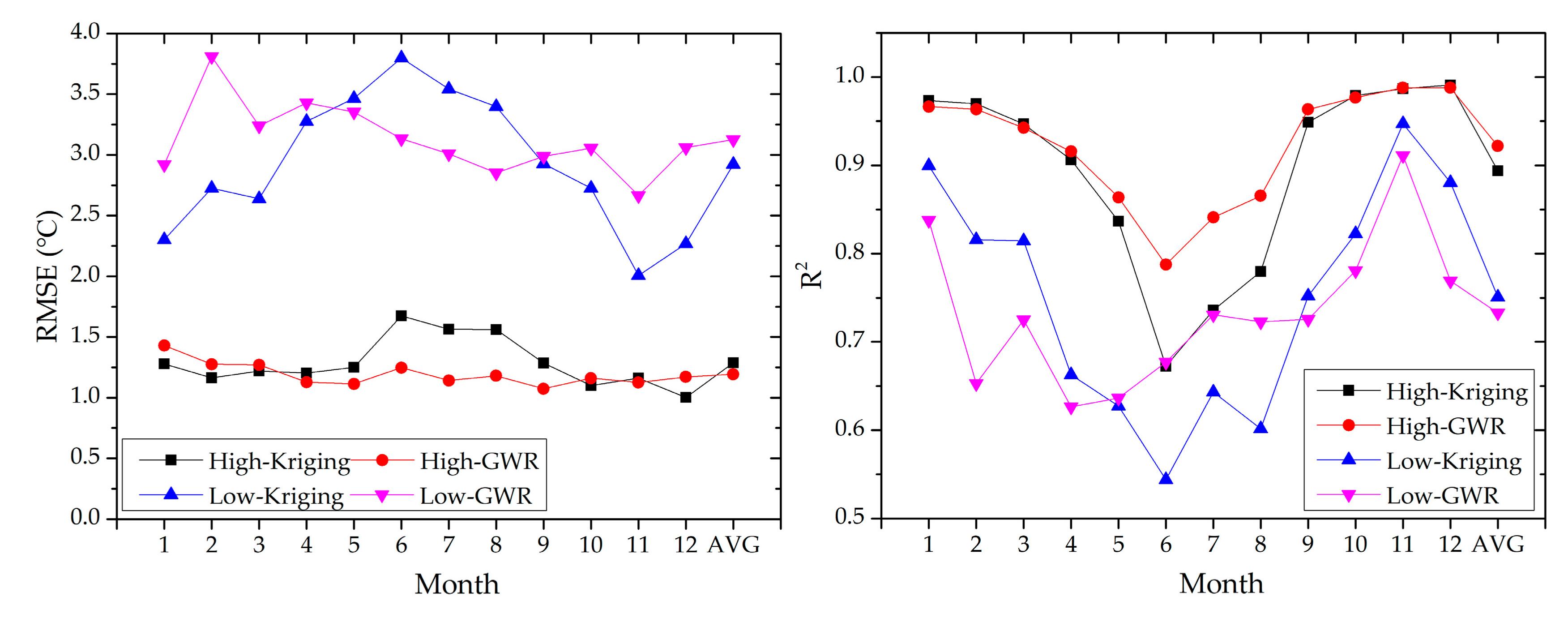
4.4. Comparison between Varied Weather Station Densities
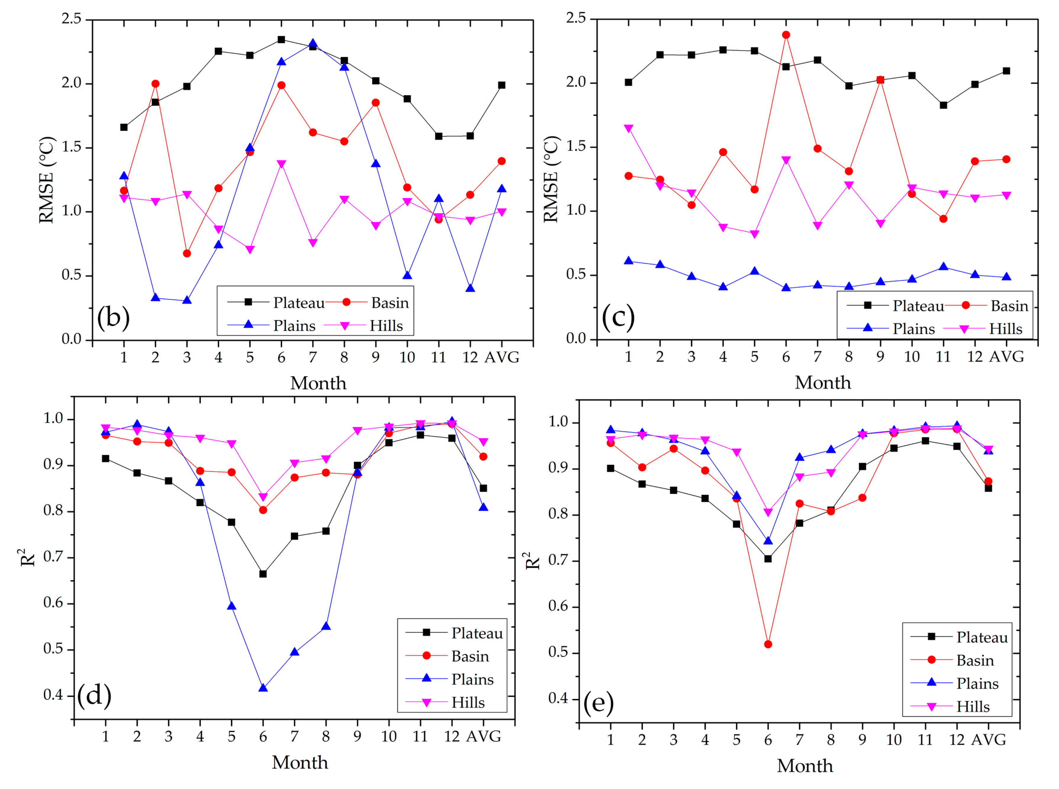
4.5. Comparison between Different Terrain Types
5. Discussion
6. Conclusions
Acknowledgments
Author Contributions
Conflicts of Interest
References
- Guan, H.; Zhang, X.; Makhnin, O.; Sun, Z. Mapping mean monthly temperatures over a coastal hilly area incorporating terrain aspect effects. J. Hydrometeorol. 2013, 14, 233–250. [Google Scholar] [CrossRef]
- Hansen, J.; Sato, M.; Ruedy, R.; Lo, K.; Lea, D.W.; Medina-Elizade, M. Global temperature change. Proc. Natl. Acad. Sci. USA 2006, 103, 14288–14293. [Google Scholar] [CrossRef] [PubMed]
- Zhu, W.; Lű, A.; Jia, S. Estimation of daily maximum and minimum air temperature using modis land surface temperature products. Remote Sens. Environ. 2013, 130, 62–73. [Google Scholar] [CrossRef]
- Yang, J.; Tan, C.; Zhang, T. Spatial and temporal variations in air temperature and precipitation in the chinese himalayas during the 1971–2007. Int. J. Clim. 2012, 33, 2622–2632. [Google Scholar] [CrossRef]
- Ge, Q.; Zhang, X.; Zheng, J. Simulated effects of vegetation increase/decrease on temperature changes from 1982 to 2000 across the eastern china. Int. J. Clim. 2014, 34, 187–196. [Google Scholar] [CrossRef]
- Fu, G.; Shen, Z.; Zhang, X.; Shi, P.; Zhang, Y.; Wu, J. Estimating air temperature of an alpine meadow on the northern tibetan plateau using modis land surface temperature. Acta Ecol. Sin. 2011, 31, 8–13. [Google Scholar] [CrossRef]
- Xu, Y.; Knudby, A.; Ho, H.C. Estimating daily maximum air temperature from modis in british columbia, Canada. Int. J. Remote Sens. 2014, 35, 8108–8121. [Google Scholar] [CrossRef]
- Cristóbal, J.; Ninyerola, M.; Pons, X. Modeling air temperature through a combination of remote sensing and gis data. J. Geophys. Res. 2008, 113, D13106. [Google Scholar] [CrossRef]
- Cristóbal, J.; Ninyerola, M.; Pons, X.; Pla, M. Improving air temperature modelization by means of remote sensing variables. In Proceedings of the 2006 IEEE International Symposium on Geoscience and Remote Sensing, Denver, CO, USA, 31 July–4 August 2006; pp. 2251–2254. [Google Scholar]
- Ninyerola, M.; Pons, X.; Roure, J.M. Objective air temperature mapping for the iberian peninsula using spatial interpolation and gis. Int. J. Clim. 2007, 27, 1231–1242. [Google Scholar] [CrossRef]
- El Kenawy, A.; López-Moreno, J.I.; Vicente-Serrano, S.M.; Morsi, F. Climatological modeling of monthly air temperature and precipitation in egypt through gis techniques. Clim. Res. 2010, 42, 161–176. [Google Scholar] [CrossRef]
- Chen, F.; Liu, Y.; Liu, Q.; Qin, F. A statistical method based on remote sensing for the estimation of air temperature in China. Int. J. Clim. 2015, 35, 2131–2143. [Google Scholar] [CrossRef]
- Evrendilek, F.; Karakaya, N.; Gungor, K.; Aslan, G. Satellite-based and mesoscale regression modeling of monthly air and soil temperatures over complex terrain in turkey. Expert Syst. Appl. 2012, 39, 2059–2066. [Google Scholar] [CrossRef]
- Bennie, J.; Wiltshire, A.; Joyce, A.; Clark, D.; Lloyd, A.; Adamson, J.; Parr, T.; Baxter, R.; Huntley, B. Characterising inter-annual variation in the spatial pattern of thermal microclimate in a uk upland using a combined empirical–physical model. Agric. For. Meteorol. 2010, 150, 12–19. [Google Scholar] [CrossRef]
- Pape, R.; Wundram, D.; Löffler, J. Modelling near-surface temperature conditions in high mountain environments: An appraisal. Clim. Res. 2009, 39, 99–109. [Google Scholar] [CrossRef]
- Gholamnia, M.; Alavipanah, S.K.; Darvishi Boloorani, A.; Hamzeh, S.; Kiavarz, M. Diurnal air temperature modeling based on the land surface temperature. Remote Sens. 2017, 9, 915. [Google Scholar] [CrossRef]
- Zhou, W.; Peng, B.; Shi, J.; Wang, T.; Dhital, Y.; Yao, R.; Yu, Y.; Lei, Z.; Zhao, R. Estimating high resolution daily air temperature based on remote sensing products and climate reanalysis datasets over glacierized basins: A case study in the langtang valley, Nepal. Remote Sens. 2017, 9, 959. [Google Scholar] [CrossRef]
- Good, E. Daily minimum and maximum surface air temperatures from geostationary satellite data. J. Geophys. Res. Atmos. 2015, 120, 2306–2324. [Google Scholar] [CrossRef]
- Peón, J.; Recondo, C.; Calleja, J.F. Improvements in the estimation of daily minimum air temperature in peninsular spain using modis land surface temperature. Int. J. Remote Sens. 2014, 35, 5148–5166. [Google Scholar] [CrossRef]
- Sun, Y.-J.; Wang, J.-F.; Zhang, R.-H.; Gillies, R.; Xue, Y.; Bo, Y.-C. Air temperature retrieval from remote sensing data based on thermodynamics. Theor. Appl. Clim. 2005, 80, 37–48. [Google Scholar] [CrossRef]
- Niclos, R.; Valiente, J.; Barbera, M.J.; Caselles, V. Land surface air temperature retrieval from eos-modis images. IEEE Geosci. Remote Sens. Lett. 2014, 11, 1380–1384. [Google Scholar] [CrossRef]
- GLass, G. Integrating avhrr satellite data and noaa ground observations to predict surface air temperature: A statistical approach. Int. J. Remote Sens. 2004, 25, 2979–2994. [Google Scholar]
- Hou, P.; Chen, Y.; Qiao, W.; Cao, G.; Jiang, W.; Li, J. Near-surface air temperature retrieval from satellite images and influence by wetlands in urban region. Theor. Appl. Clim. 2013, 111, 109–118. [Google Scholar] [CrossRef]
- Stahl, K.; Moore, R.; Floyer, J.; Asplin, M.; McKendry, I. Comparison of approaches for spatial interpolation of daily air temperature in a large region with complex topography and highly variable station density. Agric. For. Meteorol. 2006, 139, 224–236. [Google Scholar] [CrossRef]
- Benavides, R.; Montes, F.; Rubio, A.; Osoro, K. Geostatistical modelling of air temperature in a mountainous region of northern spain. Agric. For. Meteorol. 2007, 146, 173–188. [Google Scholar] [CrossRef]
- Duhan, D.; Pandey, A.; Gahalaut, K.P.S.; Pandey, R.P. Spatial and temporal variability in maximum, minimum and mean air temperatures at madhya pradesh in central india. C. R. Geosci. 2013, 345, 3–21. [Google Scholar] [CrossRef]
- Vogt, J.; Viau, A.A.; Paquet, F. Mapping regional air temperature fields using satelliteiteaximum, minimum and mean air temp. Int. J. Clim. 1997, 17, 1559–1579. [Google Scholar] [CrossRef]
- Stisen, S.; Sandholt, I.; Nørgaard, A.; Fensholt, R.; Eklundh, L. Estimation of diurnal air temperature using msg seviri data in west africa. Remote Sens. Environ. 2007, 110, 262–274. [Google Scholar] [CrossRef]
- Nieto, H.; Sandholt, I.; Aguado, I.; Chuvieco, E.; Stisen, S. Air temperature estimation with msg-seviri data: Calibration and validation of the tvx algorithm for the iberian peninsula. Remote Sens. Environ. 2011, 115, 107–116. [Google Scholar] [CrossRef]
- Kawashima, S.; Ishida, T.; Minomura, M.; Miwa, T. Relations between surface temperature and air temperature on a local scale during winter nights. J. Appl. Meteorol. 2000, 39, 1570–1579. [Google Scholar] [CrossRef]
- Cheng, K.; Su, Y.; Kuo, F.; Hung, W.; Chiang, J. Assessing the effect of landcover changes on air temperature using remote sensing images—A pilot study in northern Taiwan. Landsc. Urban Plan. 2008, 85, 85–96. [Google Scholar] [CrossRef]
- Fotheringham, A.S.; Brunsdon, C.; Charlton, M. Geographically Weighted Regression: The Analysis of Spatially Varying Relationships; John Wiley & Sons: New York, NY, USA, 2003; pp. 272–275. [Google Scholar]
- Foody, G. Geographical weighting as a further refinement to regression modelling: An example focused on the ndvi—Rainfall relationship. Remote Sens. Environ. 2003, 88, 283–293. [Google Scholar] [CrossRef]
- Peng, B.; Zhou, Y.; Gao, P.; Ju, W. Suitability assessment of different interpolation methods in the gridding process of station collected air temperature: A case study in Jiangsu province, China. J. Geo-Inf. Sci. 2011, 13, 539–548. [Google Scholar]
- Zhao, C.; Nan, Z.; Cheng, G. Methods for modelling of temporal and spatial distribution of air temperature at landscape scale in the southern Qilian mountains, China. Ecol. Model. 2005, 189, 209–220. [Google Scholar]
- Wan, Z.; Dozier, J. A generalized split-window algorithm for retrieving land-surface temperature from space. IEEE Trans. Geosci. Remote Sens. 1996, 34, 892–905. [Google Scholar]
- Wan, Z. New refinements and validation of the collection-6 modis land-surface temperature/emissivity product. Remote Sens. Environ. 2014, 140, 36–45. [Google Scholar] [CrossRef]
- Wan, Z.; Li, Z.-L. A physics-based algorithm for retrieving land-surface emissivity and temperature from eos/modis data. IEEE Trans. Geosci. Remote Sens. 1997, 35, 980–996. [Google Scholar]
- Laads Daac. Available online: https://ladsweb.modaps.eosdis.nasa.gov/search/ (accessed on 29 November 2017).
- National Meteorological Information Center. Available online: http://data.cma.cn/ (accessed on 29 November 2017).
- Srtm 90m Digital Elevation Database v4.1. Available online: http://www.cgiar-csi.org/data/%20srtm-90m-digital-elevation-database-v4-1 (accessed on 29 November 2017).
- An Overview of the Interpolation Toolset. Available online: http://resources.arcgis.com/en/help/main/10.2/index.html#/An_overview_of_the_Interpolation_tools/009z00000069000000/ (accessed on 29 November 2017).
- Zheng, X.; Zhu, J.; Yan, Q. Monthly air temperatures over northern china estimated by integrating modis data with gis techniques. J. Appl. Meteorol. Clim. 2013, 52, 1987–2000. [Google Scholar] [CrossRef]


© 2017 by the authors. Licensee MDPI, Basel, Switzerland. This article is an open access article distributed under the terms and conditions of the Creative Commons Attribution (CC BY) license (http://creativecommons.org/licenses/by/4.0/).
Share and Cite
Wang, M.; He, G.; Zhang, Z.; Wang, G.; Zhang, Z.; Cao, X.; Wu, Z.; Liu, X. Comparison of Spatial Interpolation and Regression Analysis Models for an Estimation of Monthly Near Surface Air Temperature in China. Remote Sens. 2017, 9, 1278. https://doi.org/10.3390/rs9121278
Wang M, He G, Zhang Z, Wang G, Zhang Z, Cao X, Wu Z, Liu X. Comparison of Spatial Interpolation and Regression Analysis Models for an Estimation of Monthly Near Surface Air Temperature in China. Remote Sensing. 2017; 9(12):1278. https://doi.org/10.3390/rs9121278
Chicago/Turabian StyleWang, Mengmeng, Guojin He, Zhaoming Zhang, Guizhou Wang, Zhengjia Zhang, Xiaojie Cao, Zhijie Wu, and Xiuguo Liu. 2017. "Comparison of Spatial Interpolation and Regression Analysis Models for an Estimation of Monthly Near Surface Air Temperature in China" Remote Sensing 9, no. 12: 1278. https://doi.org/10.3390/rs9121278
APA StyleWang, M., He, G., Zhang, Z., Wang, G., Zhang, Z., Cao, X., Wu, Z., & Liu, X. (2017). Comparison of Spatial Interpolation and Regression Analysis Models for an Estimation of Monthly Near Surface Air Temperature in China. Remote Sensing, 9(12), 1278. https://doi.org/10.3390/rs9121278