Article

Reduced Methane Emissions from Santa Barbara Marine Seeps

1
Institute of Environmental Physics, University of Bremen, FB 1, P.O. Box 330440, D-28334 Bremen, Germany
2
Bubbleology Research International (BRI), Solvang, CA 93463, USA
3
Earth Science Division, NASA Ames Research Center (ARC), Mountain View, CA 94035, USA
4
Center for Interdisciplinary Remotely-Piloted Aircraft Studies (CIRPAS), Marina, CA 93933, USA
*
Author to whom correspondence should be addressed.
Remote Sens. 2017, 9(11), 1162; https://doi.org/10.3390/rs9111162
Submission received: 1 September 2017 / Revised: 14 October 2017 / Accepted: 2 November 2017 / Published: 13 November 2017
(This article belongs to the Special Issue Remote Sensing of Greenhouse Gases)

Abstract

:
Airborne in situ and remote sensing measurements of methane were performed over the marine seeps in the Santa Barbara Channel close to the Coal Oil Point in California on two days in June and August 2014 with the aim to re-assess their methane emissions. During this period, methane column averaged dry air mole fractions derived from airborne remote sensing measurements in the short-wave infrared and airborne in situ measurements of methane indicate that emissions are 2–6 kt CH 4 y 1 , significantly lower than expected from previous publications. This is also confirmed by the on ground in situ measurement time series recorded at the onshore West Campus Monitoring Station in Santa Barbara. Using a time series of methane data, a decline in methane concentrations between 2008 and 2015 of more than a factor of two was derived for air masses originating from the seep field direction.

Graphical Abstract

1. Introduction

Methane, CH 4 , is the second most important greenhouse gas whose atmospheric concentrations are modified by anthropogenic activity, as well as by natural processes. There are many natural sources of CH 4 from biogenic (paddy fields, wetlands, bovine enteric fermentation) and geologic (diffuse fluxes over wide areas, also known as microseepage, localized flows and gas vents, both on land and on the seafloor, mud volcanoes, seeps) origins [1]. According to the most recent assessment of the global CH 4 budget [2], overall uncertainties for anthropogenic emissions appear smaller than those from natural sources. One natural source category with large uncertainties is marine geologic CH 4 seepage [2].
The seep field under investigation in this study is located in the northern Santa Barbara Channel, California, offshore of Coal Oil Point (COP), and is known to emit substantial quantities of CH 4 along with other hydrocarbon gases, oil and tar (see, for example, Allen et al. [3], Hornafius et al. [4], Leifer et al. [5]).
These seeps have been intensively studied in the past. Hydrocarbon release mechanisms and emissions have been investigated using various methodologies, including sonar [4,6], in situ methane and other hydrocarbon measurements [5,7,8,9], as well as underwater flow meters and optical bubble counters [6,10,11]. Airborne hyperspectral imaging spectroscopy has been used to map CH 4 plumes from a range of the larger seeps [12,13,14].
Figure 1 displays the main seep area visualized by sonar return measurements from 2005 [6]. It shows, for example, the strong seeps informally named ‘La Goleta’ and ‘Trilogy’, as well as the oil production platform ‘Holly’. The location of the seeps is controlled by geology—the Monterey Formation anticline and Red Mountain Fault—and several other faults and crossing faults [6]. This is why the locations and relative strengths vary little over many decades.
The marine seeps located offshore of Coal Oil Point were reported to emit about 18 kt CH 4 y 1 in total to the atmosphere, estimated using data from 1994–1996 [4] and assuming an average composition of 60% CH 4 for the direct emissions [8]. According to Bradley et al. [9], based on long-term atmospheric measurements at Coal Oil Point, emissions generally decreased until 1997 and afterwards increased at least until 2008 (the end of the analyzed time series). Wind sector analysis of these data showed significantly higher CH 4 at the measurement station from the direction of the seeps than any other direction: 2.7 ppm mean from the south versus 1.9 ppm from the west.
The COP seep field has been documented to vary on time scales from the sub-hourly [15], to tidal [16], to seasonal [9], to decadal [9,17], including explosively [5]. Sonar maps have been collected in 1972 [17], 1995 [4] and, most recently, 2005 [6]. This study provides a critical linkage between the 2005 sonar data, AVIRIS (Airborne Visible InfraRed Imaging Spectrometer) overflights in 2010 [13] and the more recent data presented herein. In this paper, we re-assess the geologic emissions of the Santa Barbara off-shore seeps. Surveys at the seep field in the northern Santa Barbara Channel were performed on two different days during the CO 2 and Methane EXperiment (COMEX) campaign: 4 June 2014 and 25 August 2014.
COMEX was a NASA- and ESA-funded campaign in support of the HyspIRI (Hyperspectral InfraRed Imager) [18] and CarbonSat [19,20] mission definition activities. It focused on strong CH 4 sources, such as oil fields [21,22] and landfills [23], among other important anthropogenic sources.

2. Materials and Methods

2.1. Instrumentation

The measurements were taken using the Center for Interdisciplinary Remotely-Piloted Aircraft Studies (CIRPAS) Twin Otter aircraft (http://www.cirpas.org/, last accessed: 14 October 2017). The measurement suite comprised the remote sensing instrument MAMAP (Methane Airborne MAPper) [24], a grating spectrometer system operated in the short-wave infrared at about 1.6 μ m for airborne column-averaged CH 4 and CO 2 observations. MAMAP has been used in the past for surveying an offshore natural gas blowout site [25], as well as onshore CH 4 from coal mine ventilation shafts [26], landfills [23] and CO 2 from coal fired power plants [27,28]. The instrument optics was mounted on a SOMAG CSM 130 gyro stabilized platform with a preselected viewing angle to capture the solar glint/glitter spot on the sea surface. The viewing angle was set manually before reaching the target area, and the yaw direction was adjusted to the direction of the solar glint using the stabilization mount. The position of the optical head was recorded by a 3DM-GX3 and a 3DM-GX1 attitude and heading reference system. Altitude was recorded via GPS. This information was taken into account in the determination of measurement geolocation. In glint mode over water, the expected precision of the retrieved column-averaged CH 4 is about 0.25% relative to the background CH 4 column [25].
In addition, the following instruments were installed: a G-2301f Picarro fast in situ greenhouse gas analyzer (CH 4 , CO 2 , H 2 O) provided by the NASA Ames Research Center (ARC); a radome 5-hole turbulence probe and an atmospheric measurement package operated by CIRPAS measuring wind, aerosols, temperature, dew-point and pressure.
The G-2301f Picarro greenhouse gas in situ analyzer collected measurements of CH 4 , CO 2 and H 2 O at 0.5 Hz. The H 2 O measurements are used by the software of the analyzer to automatically compute dry gas mole fractions of CH 4 and CO 2 (see Rella et al. [29] and the references therein). Before any further analysis, these dry gas mole fractions are corrected by their calibration factors for CO 2 (1.004664623) and CH 4 (1.002275041). The calibration factors were derived from measurements of known National Oceanic and Atmospheric Administrations (NOAA) standards. Based on laboratory experiments, the uncertainties of the dry gas mole fractions were estimated to be 0.15 ppm (for CO 2 ) and 2.3 ppb (for CH 4 ), which is relatively small compared to the CH 4 enhancements usually observed. Additionally, the measurements were corrected for a time lag/delay. This is achieved by accounting for the time that it takes an air sample after entering the atmospheric in situ sampling boom of the aircraft to reach the actual measurement cell in the cavity of the Picarro instrument. The time lag was estimated at 21 s (±5 s) [23]. Neglecting this time lag would introduce a location error of over 1 km assuming an aircraft speed of around 60 m · s 1 .
The measurement strategy involved flying a remote sensing pattern above the boundary layer and a ‘wall’ of in situ measurements with flight legs at different altitudes downwind of the main sources. In addition, ground-based data were analyzed, recorded at the West Campus Station (WCS) located 1 km almost due north of Coal Oil Point (34.414959°N, 119.879641°W), about 200 m west of Devereaux Slough, which drains to the southwest. WCS is situated at an altitude of 11 m (winds and air samples at 10 m above ground). Coal Oil Point has 10-m bluffs overlooking the Pacific, with the terrain rising slightly to approximately 20 m to the west and with two large petroleum storage tanks about 200 m to the northeast. Given the local topography and proximity to the shoreline, winds measured at WCS are likely highly similar to offshore winds.
To provide temporal context, the WCS time series data for wind direction, wind speed and total hydrocarbon (THC) from 2008–2015 were analyzed. THC is measured using a flame ionization detector (FID). Details on WCS are provided in Leifer et al. [5] and Bradley et al. [9]. Seep field gas that has transited the water column and escaped to the atmosphere is comprised mostly of CH 4 [5]. Data are recorded every minute, and were first filtered using a rolling-average (low-pass, 3-min, filter), with THC < 1.6 ppm classified as outliers (generally from when the system switches between sample air and calibration gas). Low-pass filtering of winds was applied separately to the north and east components.
To highlight longer timescale variations, winds in a rolling 2-week window with 86% overlap were segregated in 10° wind direction bins, with 80% overlap, and averaged. The direction, θ , and time, t, resolved THC( θ ,t) then was segregated and averaged across the seep directions (100° < θ < 250°) and across the background directions (30° < θ < 70° and 275° < θ < 360°). The latter track changes in ambient CH 4 concentrations in the Santa Barbara Basin from regional and global trends.

2.2. Inversion of In Situ Data

In situ data were gathered on different altitude legs downwind of the sources. To infer emission rates from these data, an inversion method based on a mass balance approach was applied. The key steps of this approach comprise (1) the projection of measurements along the flight track onto a plane surface, which is approximately perpendicular to the mean wind direction in the area during the flight, (2) the interpolation of measurements including assumptions of, for example, concentrations at the sea surface and top of the boundary layer and (3) the calculation of the CH 4 flux through the plane surface.
The interpolation relies on a kriging approach (see Krautwurst et al. [23] for details), which is used to fill the gaps between the flight legs. To account for the lack of measurements at the sea surface, a pseudo surface track was added. This track mimics the measurements of the two most important parameters, concentration and wind speed acquired along the lowest ‘real’ flight leg. In the same manner, a pseudo track was added at the estimated top of the boundary layer. For the subsequent flux estimate, the excess CH 4 due to the emissions of the seep field is needed. Therefore, on each side of the ‘seep field plume’, a background area was defined, which was used to estimate the CH 4 background concentrations in that area on the respective flight day. Subsequently, this 2D background concentration field was subtracted from the interpolated concentration field yielding the CH 4 concentration above the local background used in the mass balance approach.
The considered error sources are uncertainties in the boundary layer height, the plume extrapolation to the ocean surface and the top of the boundary layer, wind speed, CH 4 background concentration, the time lag and the selection of kriging parameters.

2.3. Retrieval of MAMAP Remote Sensing Data

Data analysis and retrieval of the column-averaged dry air mole fractions of methane (XCH 4 ) were performed using the weighting function modified differential optical absorption spectroscopy (WFMDOAS) algorithm as described in detail in Krings et al. [26,27] using carbon dioxide as a light path proxy (denoted as XCH 4 [CO 2 ]). The proxy method [30,31] accounts for light path variations that may occur, for example in the presence of aerosols or sub-visual cirrus. These variations largely cancel for the ratio of observations that are spectrally close to one another (see Krings et al. [26,27] and the references therein).
To account for the special geometry and reflectance behavior for sun glint in the retrieval, the SCIATRAN radiative transfer model [32] was operated in sun glint mode, applying the glint parameterization of Cox and Munk [33]. To reduce observations that missed the sun glint spot and to ensure a sufficient signal to noise ratio, measurements were only accepted for further processing provided detector filling was at least 20% of the full well capacity (in line with Krings et al. [28]). Additionally, measurements were removed when the viewing angle deviated more than 2° from the prescribed value, e.g., when the aircraft was turning.
The background column for background normalization of the remote sensing data is defined as being the dry mole fraction of the gases for regions close to the target, which are not directly affected by the seeps, based on in situ measurements. It is assumed that in situ observations made above the atmospheric boundary layer characterize the free troposphere. For the two layers, free troposphere and boundary layer, the median for CH 4 and CO 2 was calculated from the in situ measurements. Subsequently, these values were used to scale the U.S. standard atmosphere profiles of CO 2 and CH 4 to the current conditions.

2.4. Gaussian Forward Model

A Gaussian forward model was applied to compare the actual measurements with the expectations. The simulations were performed applying a vertically-integrated Gaussian plume model [27] and emission rates of 18 kt CH 4 y 1 [4], while assuming an average composition of 60% CH 4 at the sea surface, accounting for dissolution in the water column [8]. We took a simplified approach by assuming that all emissions from the seep field originated from the two main seep areas, Trilogy and La Goleta, which were enlarged to 1500 m in diameter.

3. Results

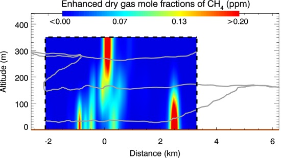
3.1. Airborne Measurements from 4 June 2014

Airborne measurements on 4 June 2014 over the Coal Oil Point seep field were performed between 11:35 and 14:30 local time.
When inspecting the airborne in situ CH 4 measurements (see Figure 2 and Figure 3), maximum enhancements in the signal of about 6% (or 0.12 ppm) in the lower boundary layer downwind of the seeps are observed. The exact boundary layer depth is difficult to assess from in situ observations as the aerosol profile indicates a strong change at 250 m, whereas potential temperature indicates a depth of about 150 m (see Figure 4). The height of 250 m, where there were also no more elevated CH 4 concentrations measured, was therefore used as a conservative estimate (i.e., leading to higher, inferred emission rates) for the boundary layer depth and the maximum plume height.
To estimate the expected relative total column enhancement from the in situ enhancements measured in the boundary layer, the kriged data yielding interpolated CH 4 enhancements (see Figure 5) were used. Assuming a boundary layer depth of 250 m, the maximum relative total column enhancement was estimated at about 0.12%.
This estimate is well below what was predicted by the Gaussian plume simulations with peak relative column enhancements of about +0.8%, indicating that the emissions at the time of the overpass were a factor of approximately seven less than the 18 kt CH 4 y 1 .
This is also confirmed by the more rigorous approach to compute a flux from the in situ measurements using the mass balance approach as described in Section 2.2 and using the estimated top of the boundary layer of 250 m. The measured CH 4 and interpolated enhancements are shown in Figure 5. The resulting emission rate was estimated to be about 1.6 kt CH 4 y 1 , which is approximately an order of magnitude lower than originally expected. The corresponding uncertainty is about 41%. A list of all error contributions considered and further details are listed in Table 1.
The remote sensing measurements (Figure 6) were performed between 11:35 and 13:45 local time. Aircraft altitude was 1400 m above sea level, resulting in an observed ground scene size of about 65 m × 60 m (cross track × along track) for one observation. The background columns were about 1.810 ppm for XCH 4 and about 401.2 ppm for XCO 2 .
Quality filtered data and the corresponding retrieved background normalized XCH 4 [CO 2 ] data are shown in Figure 6 (left). Given the wind direction of about 247° at 3.5 m·s 1 (derived from the CIRPAS wind probe; see Appendix A), there is no plume structure of XCH 4 visible downwind of the main seep areas, which are indicated in the plot by the two black crosses. The crosses represent the seabed center locations of the prominent Trilogy (northwest) and the La Goleta (southeast) seeps, which are the largest seeps in the Coal Oil Point area. Deviations at the sea surface due to currents are at most 30 m given typical currents and the water depths.
Also shown are the solar zenith angles (SZA) for each measurement time and location (Figure 6, right), indicating that the SZA varied from about 11–22° during the survey, but that the preset inclination angle of about 12° was well suited for most measurements.
To support the assumption that the CH 4 from the seeps should have been observed by MAMAP provided the source strength was similar to that reported in Hornafius et al. [4], simulations were performed applying the Gaussian plume model. Winds were about 3.5 m·s 1 from 247° as derived from CIRPAS observations. The atmospheric stability was determined to be ‘moderately unstable’ based on Hasse et al. [34] and temperature data from the National Oceanic and Atmospheric Association (NOAA) (http://www.ndbc.noaa.gov/station_history.php?station=46053).
The results gridded to 100 m × 100 m are shown in Figure 7 and indicate that a clear signal is expected that should have been visible also in the presence of typical instrument measurement noise. The precision of retrieved XCH 4 was about 0.18% (1 σ ) evaluated as the standard deviation from the data and is similar to MAMAP glint observations at the North Sea from 2011 [25].

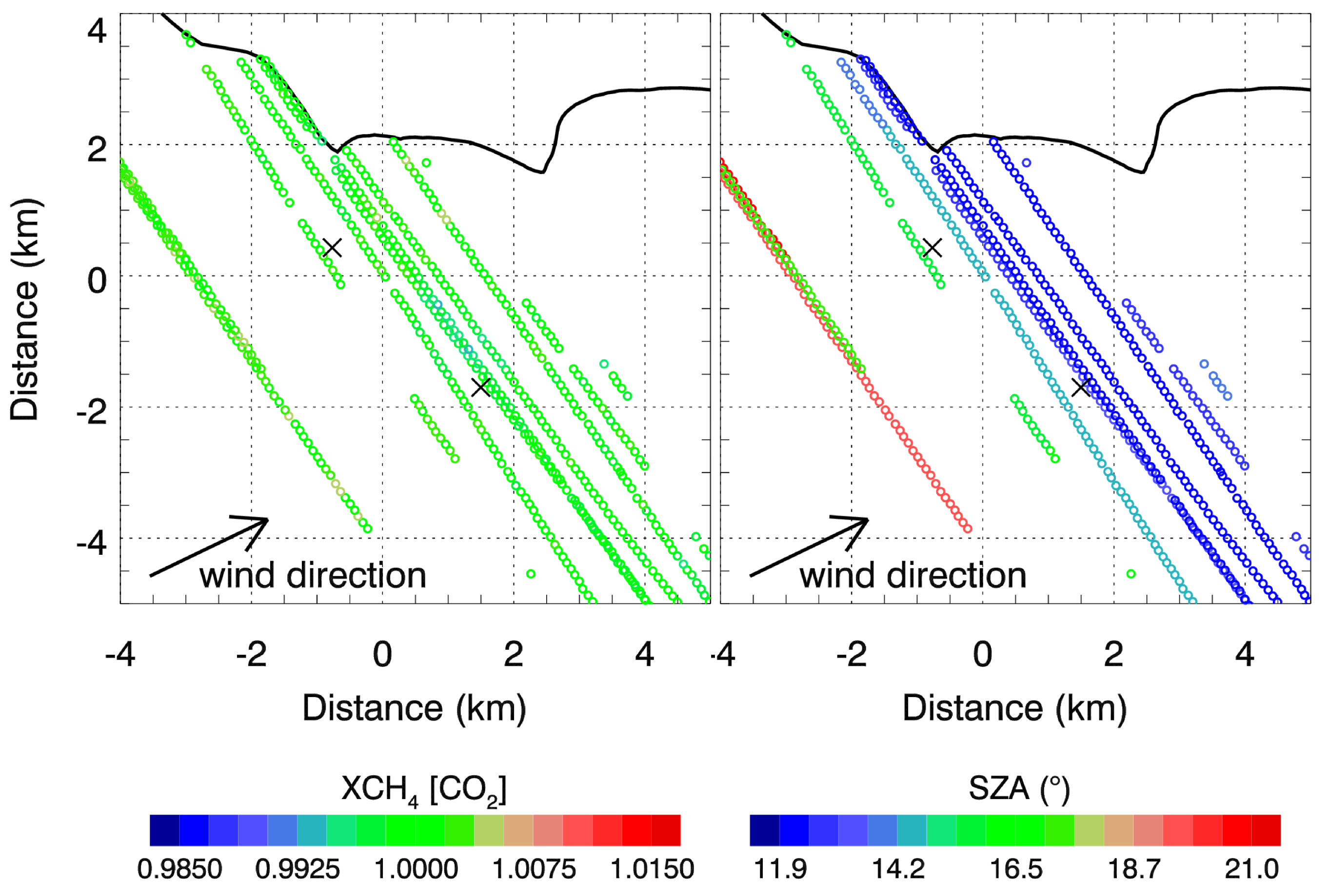
3.2. Airborne Measurements from 25 August 2014

The airborne in situ measurements for this day show strong, local increases in CH 4 , downwind of Trilogy and La Goleta Seep (see Figure 8 and Figure 9) with a maximum of about 0.48 ppm above the background (+25%) close to the sea surface downwind of La Goleta seep. There is no clear plume structure apparent in the in situ data. Whereas the highest in situ flight line shows significant enhancements in CH 4 downwind of the Trilogy seep area, the remote sensing flight track shows no enhancement; however, this is too high to give a reasonable vertical constraint. The lack of vertical extent constraint introduces uncertainty in the column estimate. The boundary layer depth was estimated using the potential temperature and aerosol profile showing well-mixed conditions to about 300–350 m (see Figure 10). Assuming the enhancement of the third flight line is representative of a boundary layer depth of about 350 m, the maximum total column increase is about 0.31%. This enhancement was derived from the vertically-integrated enhancements on the kriged data (see Figure 11), which provides an approximate CH 4 distribution within the atmospheric boundary layer.
This estimated column enhancement is below the conservative maximum enhancements expected from plume simulations (assumed wind from 260° at 5.3 m·s 1 ; see Appendix A), which predicted peak enhancements of about 0.5% close to the source.
A mass balance inversion of the in situ data was calculated for this day. The interpolated CH 4 measurements that were used for the flux inversion are shown in Figure 11 (right). The resulting emissions for the area were estimated at about 5.1 kt CH 4 y 1 . The uncertainty of the emission rate was estimated in a similar manner to that for 4 June 2014 and is about 19% (see Table 1).
The MAMAP measurements on 25 August 2014 over the Coal Oil Point area were performed from about 12:30–15:15 local time. Aircraft altitude for the remote sensing measurements was about 2060 m, and the MAMAP instrument was mounted with a preselected viewing angle of 25.0° to capture the solar glint/glitter spot on the sea. The viewing angle was manually pre-set before reaching the target area and (manually) adjusted once during the flight to 28.5°. The observed ground scene size was about 115 m × 90 m (cross track × along track). The background dry mole fractions were about 1.797 ppm for XCH 4 and about 391.2 ppm for XCO 2 derived from Picarro in situ measurements.
When inspecting the MAMAP remote sensing measurements for this flight, it becomes clear that the detector was measuring mostly below 10% of the full well capacity in the second part of the flight (see Figure 12, left). The main reason is that the glint spot was not perfectly aligned for the measurements performed in the second part, leading to a low signal and also low signal to noise ratio. In Figure 12 (center), the change in solar zenith angle during the survey is shown spanning a range from about 23–39°, whereas the preselected viewing angle was manually set to 25.0° (and later to 28.5°).
To allow at least qualitative inspection of the low signal data, the measurements were additionally smoothed by applying a normalization of a 100-point moving average, which otherwise is generally not necessary when analyzing MAMAP data, e.g., for derivation of emission rates. Furthermore, a basic signal filter was applied (5% of the full well capacity) in addition to the inclination filter (±2° as for 4 June 2014). The resulting, qualitative XCH 4 [CO 2 ] map is shown in Figure 12 (right).
No significant CH 4 enhancements downwind of the sources are visible. However, considering, for example, atmospheric variability, the two downwind flight lines are not sufficient to clearly identify (or exclude) potential methane plumes originating at the two seep locations.

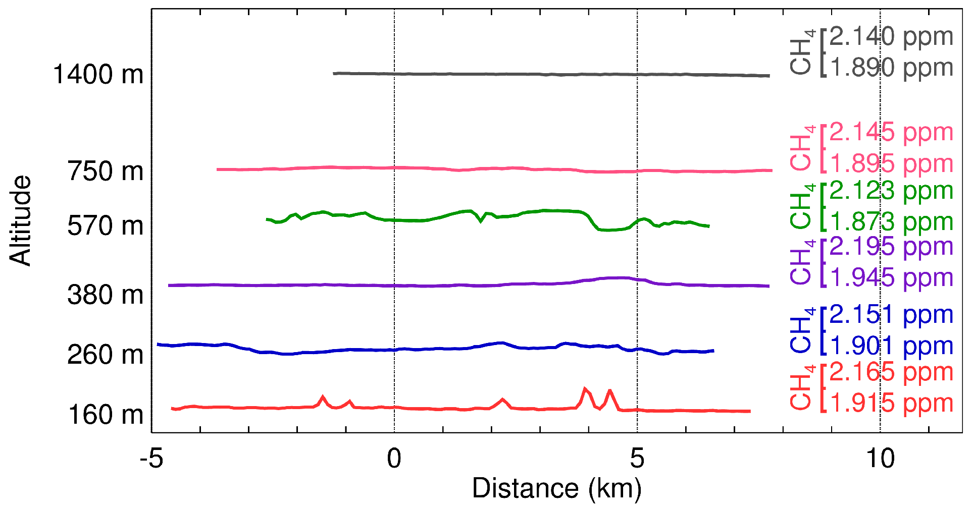
3.3. Ground Based In Situ Measurements

The time series from the seep directions recorded at West Campus Station (WCS) (see Figure 13) showed a clear seasonal cycle with lower seep field direct concentrations in summer than winter. Also apparent is a decreasing trend from 2008–2015. This decrease is stronger in the anomaly (seep direction-background) trend, THC’ (see Figure 13, bottom). A linear polynomial least squares linear regression analysis of THC’(t) found a decrease from 0.37 ppm in 2008 to 0.15 ppm at the beginning of 2015, more than a factor of two. Given that WCS winds over this period did not show interannual changes [9], this corresponds directly to similar emission changes. Summer emissions are significantly less than the annual average, and there also are far fewer large transient releases in summer than winter.

4. Discussion

The in situ inversion results show 10-times (4 June 2014) and three-times (25 August 2014) lower emissions than originally expected for the seep area. The emission rate estimate based on the June measurements, 1.6 kt CH 4 y 1 (±41%), shows a rather high uncertainty due to the increased uncertainty in the boundary layer depth resulting from a mismatch between the two indicators: aerosol and potential temperature. This could be, for example, due to a residual layer. The baseline of 250 m boundary layer depth was selected as a conservative estimate leading to a relatively higher, but absolutely still very low emission rate estimate.
Based on the experience gained from the first flight, the flight patterns on 25 August 2014 were optimized for lower flight altitudes starting from the lowest flight leg. However, as campaign flights were focused primarily on remote sensing, the remaining flight time for in situ measurements allowed only three flight tracks at three different altitudes. In situ measurements show CH 4 enhancements on all three flight tracks within the boundary layer. However, the plume structure is not smooth, having discontinuities. This observation is in agreement with other in situ studies with several sources, for example for CO 2 emissions from power plants [28]. The resulting emission rate estimate of 5.1 kt CH 4 y 1 (±19%) is about three-times higher than on 4 June 2014, but still significantly lower than what was expected based on the literature. Additional systematic uncertainty in the total emissions arises from the fact that the plumes from the most southeastern part of the seep field were not transected (see Figure 8). Published strength estimates [6] indicate that this area has significantly lower emissions than the La Goleta Seep area. Thus, even if we assume the missing contribution accounts for 20% of total seep field emissions, the total emission rate is only about 6.4 kt CH 4 y 1 .
The case that concentrations below the lowest track may have been higher than, for example, at a 160-m altitude, on 4 June 2014 (see Figure 3) is included in the given uncertainty. However, measurements on 25 August 2014 performed at a 40-m altitude show peak concentrations comparable to the 280-m flight track (see Figure 9) indicating a rather well-mixed atmosphere at least on that day, even though there is no continuous plume structure. Note that the high values of about 200 ppm CH 4 at a 5-m altitude reported in Leifer et al. [7] were recorded directly over a bubble plume location at ‘very light’ winds with concentrations being at the background at a distance of only a few tens of meters away from the source. Concentrations close to the surface but further away from the source and during conditions of higher wind speed like in the present campaign are not expected to be anywhere close due to mixing.
The remote sensing data from 4 June 2014 do not show any plume structure. In combination with the Gaussian plume model simulations, which predicted a clear CH 4 signal observable by MAMAP, this confirms that the direct and diffuse emissions from the designated source areas were significantly lower than 18 kt CH 4 y 1 for the time of the overflight. The atmosphere might have been more stable than the assumed ‘moderately stable’ conditions leading to higher peak concentrations in the model, which would further strengthen our conclusions. The plume model is only a rough approximation, but shows that sources of the expected emission rate would have been visible with the MAMAP remote sensing instrument either by a broad plume structure or more likely higher peak values due to the more inhomogeneous source structure.
MAMAP remote sensing measurements for 25 August 2014 are not as readily used for the estimation of upper limits or actual emission rates because the flight pattern is different from 4 June 2014 due to fewer tracks downwind of the main seeps La Goleta and Trilogy. Furthermore, on this day, measurements were not taken around solar noon (unlike on 4 June 2014) with a rapidly changing solar zenith angle. In these conditions and for surveys that take longer than an hour, it is important to continuously track the sun glint spot on the ocean. This, however, was not possible with the current MAMAP instrument glint configuration. In addition, due to an underestimation of the time required to finalize the entire dense flight pattern, there is a limited number of flight tracks downwind of the seep area, which are most relevant for the detection of potential emissions.
On 4 June 2014, the aerosol load was greater compared to 25 August 2014. However, this does not impact the conclusions. The influence of aerosol on the remote sensing measurements was estimated as, for example, only 0.05% relative to the background column between urban and background aerosol [27]. Furthermore, since the effect is basically a bias and remote sensing measurements are normalized to the background, only an inhomogeneous distribution of aerosol will have an effect on the result.
In contrast to this study, much larger column enhancements for June 2008 were found via remote sensing and at a distance of about 100 m from the source of approximately 10%–20% total column above background [14]. Taking into account the weaker wind speed of about 2.5 m·s 1 [14] in contrast to 4–5 m·s 1 for this work and that measurements from this campaign were further away from the source where the plume is broader (about 500 m instead of 100 m), equivalent column enhancements to be expected are about 1.0%–2.0%, which is similar to the plume simulations using the emissions from Hornafius et al. [4]. This is significantly more than what is derived from these campaign data, both remote sensing and in situ.
Larger concentrations in 1994–1995 [4] and particularly in 2008 [14] and decreased concentrations in 2014 as found here are in agreement with the trend in ground-based in situ measurements taken at West Campus Station that were additionally analyzed for this study. The seasonal variability with reduced emissions in summer of about a factor of 2–3 relative to the mean can only partly explain the observed low emissions from the airborne experiment. The difference between emissions on the two measurement days, however, is in the range of expected variation.
In the regional context, these emissions only play a minor role. Compared to, for example, emissions in the nearby South Coast air basin, which are about 350–450 kt CH 4 y 1 [35], the seep emissions account for only about 1%.

5. Conclusions

Airborne in situ data obtained during the COMEX measurement campaign in 2014 indicate that the emission rates for the time of the overflights were significantly lower than the expected 18 kt CH 4 y 1 derived from Hornafius et al. [4] and assuming an average composition of 60% CH 4 [8]. Maximum CH 4 mole fraction enhancements observed in the boundary layer downwind of the seeps are in the range of 6% (4 June 2014) and 25% (25 August 2014) relative to the background. This leads to column enhancements of about 0.12% and about 0.31%. Emission estimates based on the airborne in situ data result in 1.6 kt CH 4 y 1 (±41%) and 5.1 kt CH 4 y 1 (6.4 kt CH 4 y 1 when accounting for the missing part) (±19%) for the two days, respectively.
A forward plume model showed expected CH 4 total column enhancements of more than 0.5% up to 0.8% for conservative ‘moderately unstable’ atmospheric conditions and an expected emission of 18 kt CH 4 y 1 . However, the MAMAP remote sensing XCH 4 data obtained on 4 June 2014 compared to the forward plume modeling indicate that emissions for the time of the overflight were significantly lower. Conclusions drawn from the 25 August 2014 remote sensing data have as a result of the flight pattern less information and are consistent (i.e., do not contradict) with the findings from the 4 June 2014.
The additional analysis of ground-based measurements taken at West Campus Station (WCS) indicates decreased emissions from the seeps. Furthermore, the WCS data show large fluctuations and inter-seasonal variations that can explain the difference in derived emissions at the two measurement days.
The combined evidence from three different types of observations indicate significantly reduced emissions to 2–6 kt CH 4 y 1 at the time of measurements from the Coal Oil Point seeps. The reasons for the decrease remain a task for further research.
The campaign and flight patterns were originally designed for a source of expected emissions of about 18 kt CH 4 y 1 . The methane enhancements produced by the significantly lower emissions were, however, below the detection limit of the MAMAP instrument. Future campaigns for such small emissions could focus more on in situ measurements, which have a higher sensitivity. However, the remote sensing data can be used to provide an upper limit, i.e., a constraint for the emissions, and to exclude cases such as having high CH 4 amounts below the lowest in situ flight track. This part of the study also demonstrates the need for next generation airborne remote sensing instruments with higher sensitivity and imaging capabilities.

Acknowledgments

We thank Laura T. Iraci from the Earth Science Division at NASA’s Ames Research Center for discussions on and support of the calibration of the airborne in situ data. The MAMAP activities are funded in part by the University and the State of Bremen, the European Space Agency (ESA) and NASA. We thank the NASA Earth Science Division, Research and Analysis Program, Grant NNX13AM21G.

Author Contributions

Heinrich Bovensmann, Ira Leifer, Konstantin Gerilowski, Sven Krautwurst, Thomas Krings, Michael Buchwitz, Matthew M. Fladeland and John P. Burrows conceived of and designed the experiment. Ira Leifer, Konstantin Gerilowski, Sven Krautwurst, Heinrich Bovensmann, Markus Horstjann, Richard W. Kolyer and Haflidi H. Jonsson made the different measurements. Thomas Krings, Konstantin Gerilowski and Sven Krautwurst analyzed the remote sensing data. Sven Krautwurst and Thomas Krings analyzed the airborne in situ data. Ira Leifer analyzed the ground-based in situ data. Thomas Krings, Ira Leifer and Sven Krautwurst wrote the paper. All authors contributed to and reviewed the paper.

Conflicts of Interest

The authors declare no conflict of interest.

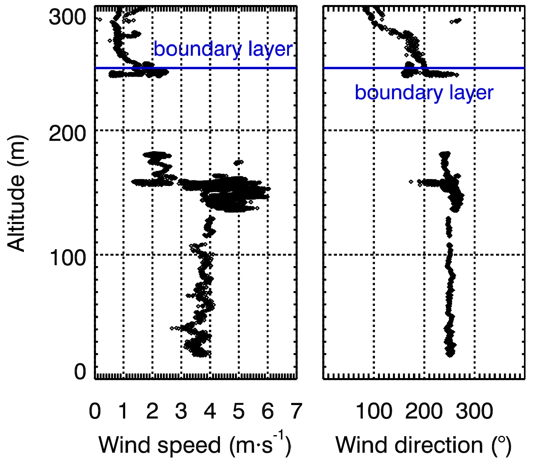
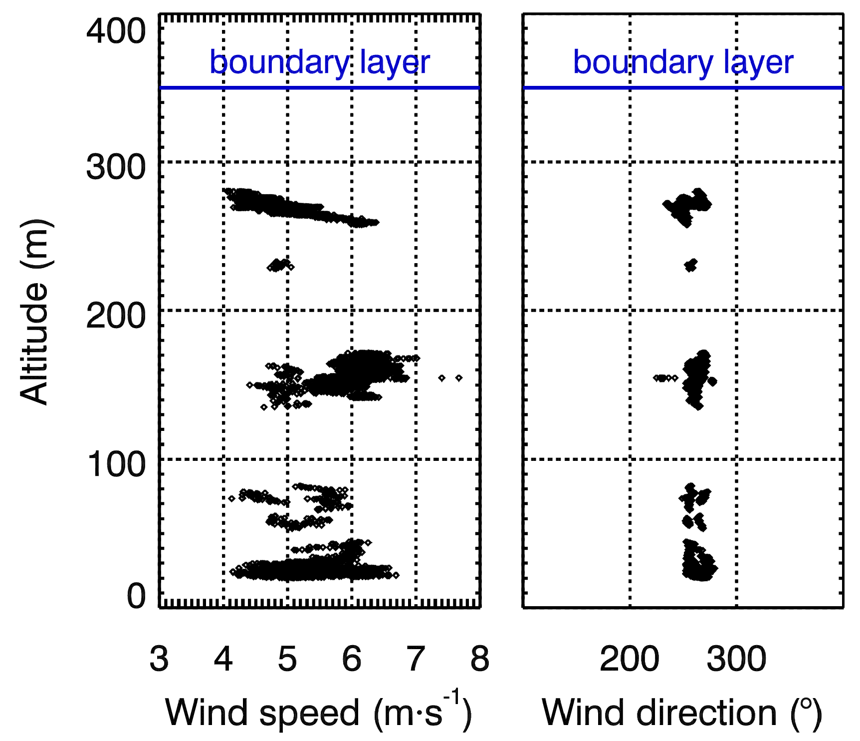
Appendix A. In Situ Wind Profiles

The wind profiles recorded by the CIRPAS in situ instrumentation are shown in Figure A1 (4 June 2014) and Figure A2 (25 August 2014). The data were filtered for inclination deviations lower than 5°. On both days, wind direction was almost constant with an altitude of about 247° on 4 June 2014 and 260° on 25 August 2014 computed from the individually averaged wind components. On 4 June 2014, wind speed appears to be somewhat higher at a 150-m altitude than below and decreasing again upwards. On 25 August 2014, wind speed varies more, but stays within the same range for all probed altitudes in the atmospheric boundary layer. The height averaged wind speed results in being about 3.5 m·s 1 on 4 June 2014 and 5.3 m·s 1 on 25 August 2014.
Figure A1. In situ wind profile measured on 4 June 2014 over the measurement area and filtered for inclination. Also indicated is the approximate boundary layer height determined for that particular day.
Remotesensing 09 01162 g0a1
Figure A2. Same as Figure A1, but for 25 August 2014.
Remotesensing 09 01162 g0a2

References

  1. Ciais, P.; Sabine, C.; Bala, G.; Bopp, L.; Brovkin, V.; Canadell, J.; Chhabra, A.; DeFries, R.; Galloway, J.; Heimann, M.; et al. Climate Change 2013: The Physical Science Basis. Contribution of Working Group I to the Fifth Assessment Report of the Intergovernmental Panel on Climate Change; Stocker, T.F., Qin, D., Plattner, G.-K., Tignor, M., Allen, S.K., Boschung, J., Nauels, A., Xia, Y., Bex, V., Midgley, P.M., Eds.; Cambridge University Press: Cambridge, UK; New York, NY, USA, 2013. [Google Scholar]
  2. Saunois, M.; Bousquet, P.; Poulter, B.; Peregon, A.; Ciais, P.; Canadell, J.G.; Dlugokencky, E.J.; Etiope, G.; Bastviken, D.; Houweling, S.; et al. The global methane budget 2000–2012. Earth Syst. Sci. Data 2016, 8, 697–751. [Google Scholar] [CrossRef]
  3. Allen, A.A.; Schlueter, R.S.; Mikolaj, P.G. Natural Oil Seepage at Coal Oil Point, Santa Barbara, California. Science 1970, 170, 974–977. [Google Scholar] [CrossRef] [PubMed]
  4. Hornafius, J.S.; Quigley, D.; Luyendyk, B.P. The world’s most spectacular marine hydrocarbon seeps (Coal Oil Point, Santa Barbara Channel, California): Quantification of emissions. J. Geophys. Res. Oceans 1999, 104, 20703–20711. [Google Scholar] [CrossRef]
  5. Leifer, I.; Luyendyk, B.P.; Boles, J.; Clark, J.F. Natural marine seepage blowout: Contribution to atmospheric methane. Glob. Biogechem. Cycles 2006, 20. [Google Scholar] [CrossRef]
  6. Leifer, I.; Kamerling, M.J.; Luyendyk, B.P.; Wilson, D.S. Geologic control of natural marine hydrocarbon seep emissions, Coal Oil Point seep field, California. Geo-Mar. Lett. 2010, 30, 331–338. [Google Scholar] [CrossRef]
  7. Leifer, I.; Roberts, D.; Margolis, J.; Kinnaman, F. In situ sensing of methane emissions from natural marine hydrocarbon seeps: A potential remote sensing technology. Earth Planet. Sci. Lett. 2006, 245, 509–522. [Google Scholar] [CrossRef]
  8. Clark, J.F.; Washburn, L.; Schwager Emery, K. Variability of gas composition and flux intensity in natural marine hydrocarbon seeps. Geo-Mar. Lett. 2009, 30, 379–388. [Google Scholar] [CrossRef]
  9. Bradley, E.; Leifer, I.; Roberts, D. Long-term monitoring of a marine geologic hydrocarbon source by a coastal air pollution station in Southern California. Atmos. Environ. 2010, 44, 4973–4981. [Google Scholar] [CrossRef]
  10. Leifer, I.; Boles, J. Measurement of marine hydrocarbon seep flow through fractured rock and unconsolidated sediment. Mar. Pet. Geol. 2005, 22, 551–568. [Google Scholar] [CrossRef]
  11. Leifer, I.; Culling, D. Formation of seep bubble plumes in the Coal Oil Point seep field. Geo-Mar. Lett. 2010, 30, 339–353. [Google Scholar] [CrossRef]
  12. Roberts, D.A.; Bradley, E.S.; Cheung, R.; Leifer, I.; Dennison, P.E.; Margolis, J.S. Mapping methane emissions from a marine geological seep source using imaging spectrometry. Remote Sens. Environ. 2010, 114, 592–606. [Google Scholar] [CrossRef]
  13. Bradley, E.S.; Leifer, I.; Roberts, D.A.; Dennison, P.E.; Washburn, L. Detection of marine methane emissions with AVIRIS band ratios. Geophys. Res. Lett. 2011, 38. [Google Scholar] [CrossRef]
  14. Thorpe, A.K.; Frankenberg, C.; Roberts, D.A. Retrieval techniques for airborne imaging of methane concentrations using high spatial and moderate spectral resolution: Application to AVIRIS. Atmos. Meas. Tech. 2014, 7, 491–506. [Google Scholar] [CrossRef]
  15. Leifer, I.; Wilson, K. The tidal influence on oil and gas emissions from an abandoned oil well: Nearshore Summerland, California. Mar. Pollut. Bull. 2007, 54, 1495–1506. [Google Scholar] [CrossRef] [PubMed]
  16. Boles, J.R.; Clark, J.F.; Leifer, I.; Washburn, L. Temporal variation in natural methane seep rate due to tides, Coal Oil Point area, California. J. Geophys. Res. Oceans 2001, 106, 27077–27086. [Google Scholar] [CrossRef]
  17. Fischer, P.J. Oil and tar seeps, Santa Barbara basin, California. In California Offshore Gas, Oil, and Tar Seeps; Fischer, P.J., Ed.; California State Lands Commission: Sacramento, CA, USA, 1978; pp. 1–62. [Google Scholar]
  18. Lee, C.M.; Cable, M.L.; Hook, S.J.; Green, R.O.; Ustin, S.L.; Mandl, D.J.; Middleton, E.M. An introduction to the {NASA} Hyperspectral InfraRed Imager (HyspIRI) mission and preparatory activities. Remote Sens. Environ. 2015, 167, 6–19. [Google Scholar]
  19. Bovensmann, H.; Buchwitz, M.; Burrows, J.P.; Reuter, M.; Krings, T.; Gerilowski, K.; Schneising, O.; Heymann, J.; Tretner, A.; Erzinger, J. A remote sensing technique for global monitoring of power plant CO2 emissions from space and related applications. Atmos. Meas. Tech. 2010, 3, 781–811. [Google Scholar] [CrossRef]
  20. Buchwitz, M.; Reuter, M.; Bovensmann, H.; Pillai, D.; Heymann, J.; Schneising, O.; Rozanov, V.; Krings, T.; Burrows, J.P.; Boesch, H.; et al. Carbon Monitoring Satellite (CarbonSat): Assessment of atmospheric CO2 and CH4 retrieval errors by error parameterization. Atmos. Meas. Tech. 2013, 6, 3477–3500. [Google Scholar] [CrossRef]
  21. Thompson, D.R.; Leifer, I.; Bovensmann, H.; Eastwood, M.; Fladeland, M.; Frankenberg, C.; Gerilowski, K.; Green, R.O.; Kratwurst, S.; Krings, T.; et al. Real-time remote detection and measurement for airborne imaging spectroscopy: A case study with methane. Atmos. Meas. Tech. 2015, 8, 4383–4397. [Google Scholar] [CrossRef]
  22. Gerilowski, K.; Krautwurst, S.; Koyler, R.; Jonsson, H.; Krings, T.; Horstjann, M.; Leifer, I.; Schuettemeyer, D.; Fladeland, M.; Burrows, J.P.; et al. Remote Sensing of Large Scale Methane Emission Sources with the Methane Airborne MAPper (MAMAP) Instrument over the Kern River and Kern Front Oil Fields and Validation through Airborne In-Situ Measurements—Initial Results from COMEX; American Geophysical Union: Washington, DC, USA, 2014. [Google Scholar]
  23. Krautwurst, S.; Gerilowski, K.; Jonsson, H.H.; Thompson, D.R.; Kolyer, R.W.; Iraci, L.T.; Thorpe, A.K.; Horstjann, M.; Eastwood, M.; Leifer, I.; et al. Methane emissions from a Californian landfill, determined from airborne remote sensing and in situ measurements. Atmos. Meas. Tech. 2017, 10, 3429–3452. [Google Scholar] [CrossRef]
  24. Gerilowski, K.; Tretner, A.; Krings, T.; Buchwitz, M.; Bertagnolio, P.P.; Belemezov, F.; Erzinger, J.; Burrows, J.P.; Bovensmann, H. MAMAP—A new spectrometer system for column-averaged methane and carbon dioxide observations from aircraft: Instrument description and performance analysis. Atmos. Meas. Tech. 2011, 4, 215–243. [Google Scholar] [CrossRef]
  25. Gerilowski, K.; Krings, T.; Hartmann, J.; Buchwitz, M.; Sachs, T.; Erzinger, J.; Burrows, J.P.; Bovensmann, H. Atmospheric remote sensing constraints on direct sea-air methane flux from the 22/4b North Sea massive blowout bubble plume. Mar. Pet. Geol. 2015, 68 Part B, 824–835. [Google Scholar] [CrossRef] [Green Version]
  26. Krings, T.; Gerilowski, K.; Buchwitz, M.; Hartmann, J.; Sachs, T.; Erzinger, J.; Burrows, J.P.; Bovensmann, H. Quantification of methane emission rates from coal mine ventilation shafts using airborne remote sensing data. Atmos. Meas. Tech. 2013, 6, 151–166. [Google Scholar] [CrossRef] [Green Version]
  27. Krings, T.; Gerilowski, K.; Buchwitz, M.; Reuter, M.; Tretner, A.; Erzinger, J.; Heinze, D.; Pflüger, U.; Burrows, J.P.; Bovensmann, H. MAMAP—A new spectrometer system for column-averaged methane and carbon dioxide observations from aircraft: Retrieval algorithm and first inversions for point source emission rates. Atmos. Meas. Tech. 2011, 4, 1735–1758. [Google Scholar] [CrossRef]
  28. Krings, T.; Neininger, B.; Gerilowski, K.; Krautwurst, S.; Buchwitz, M.; Burrows, J.P.; Lindemann, C.; Ruhtz, T.; Schüttemeyer, D.; Bovensmann, H. Airborne remote sensing and in-situ measurements of atmospheric CO2 to quantify point source emissions. Atmos. Meas. Tech. Discuss. 2016, 2016, 1–30. [Google Scholar] [CrossRef]
  29. Rella, C.W.; Chen, H.; Andrews, A.E.; Filges, A.; Gerbig, C.; Hatakka, J.; Karion, A.; Miles, N.L.; Richardson, S.J.; Steinbacher, M.; et al. High accuracy measurements of dry mole fractions of carbon dioxide and methane in humid air. Atmos. Meas. Tech. 2013, 6, 837–860. [Google Scholar]
  30. Frankenberg, C.; Meirink, J.F.; van Weele, M.; Platt, U.; Wagner, T. Assessing Methane Emissions from Global Space-Borne Observations. Science 2005, 308, 1010–1014. [Google Scholar] [CrossRef] [PubMed]
  31. Schepers, D.; Guerlet, S.; Butz, A. Methane retrievals from Greenhouse Gases Observing Satellite (GOSAT) shortwave infrared measurements: Performance comparison of proxy and physics retrieval algorithms. J. Geophys. Res. 2012, 117. [Google Scholar] [CrossRef] [Green Version]
  32. Rozanov, V.; Rozanov, A.; Kokhanovsky, A.; Burrows, J. Radiative transfer through terrestrial atmosphere and ocean: Software package {SCIATRAN}. J. Quant. Spectrosc. Radiat. Transf. 2014, 133, 13–71. [Google Scholar] [CrossRef]
  33. Cox, C.; Munk, W. Measurement of the Roughness of the Sea Surface from Photographs of the Sun’s Glitter. J. Opt. Soc. Am. 1954, 44, 838–850. [Google Scholar] [CrossRef]
  34. Hasse, L.; Weber, H. On the conversion of Pasquill categories for use over sea. Bound. Layer Meteorol. 1985, 31, 177–185. [Google Scholar] [CrossRef]
  35. Jeong, S.; Newman, S.; Zhang, J.; Andrews, A.E.; Bianco, L.; Bagley, J.; Cui, X.; Graven, H.; Kim, J.; Salameh, P.; et al. Estimating methane emissions in California’s urban and rural regions using multitower observations. J. Geophys. Res. Atmos. 2016, 121, 13031–13049. [Google Scholar] [CrossRef]
Figure 1. Seep area map with the most prominent seeps labeled, derived from sonar return measurements in 2005 [6], including La Goleta and Trilogy. The color scale shows the normalized amplitude of the sonar backscatter σ from seep bubbles. See Leifer et al. [6] for details.
Remotesensing 09 01162 g001
Figure 2. In situ CH 4 measurements from 4 June 2014. The underlying seep intensity information (red: high; green: low) is derived from sonar return data (see Leifer et al. [6]).
Remotesensing 09 01162 g002
Figure 3. Cross-section of the airborne in situ CH 4 measurements shown for the five dedicated in situ altitudes and for the closest located remote sensing track at a far higher altitude (1400 m) from 4 June 2014. The scale on the x-axis denotes the distance to the approximate location where the aircraft turns from a more east-west direction to a north-south direction (see Figure 2). Positive distances refer to measurement locations further southeast from the turning point and negative distances to locations further west from the turning point. The y-axis shows the approximate altitude of the flight lines and is not to scale, while the variations in CH 4 are according to the scales on the right, which all have the same span, but different offsets.
Remotesensing 09 01162 g003
Figure 4. Measured aerosol profile (black) and the potential temperature (blue) on 4 June 2014.
Remotesensing 09 01162 g004
Figure 5. (Left) Projected in situ measurements from 4 June 2014. Vertical, dashed lines denote the sides of the measurement area that have been used to determine the local background. The dashed box denotes the area used to derive the flux. (Right) 2D interpolated in situ CH 4 enhancements from 4 June 2014 applying a kriging approach as used in Krautwurst et al. [23]. The dashed black line outlines the area used for the flux calculation. The x-axis is similar to Figure 3, but for the projected measurements.
Remotesensing 09 01162 g005
Figure 6. (Left) Column-averaged dry air mole fraction of methane, XCH 4 , derived from MAMAP remote sensing data for 4 June 2014, normalized by a regional mean and displayed relative to the background. (Right) The corresponding solar zenith angle (SZA) for each data point. Crosses mark the approximate center locations of the Trilogy and La Goleta seep areas.
Remotesensing 09 01162 g006
Figure 7. Gaussian plume model simulations with random noise for two equal sources of 1500 m in width and a total source strength of 18 kt CH 4 y 1 located at the approximate locations of the Trilogy and La Goleta seeps and using the flight path for 4 June 2014.
Remotesensing 09 01162 g007
Figure 8. In situ CH 4 measurements from 25 August 2014. The underlying seep intensity information (red: high; green: low) is derived from sonar data from 2005 (see Leifer et al. [6]).
Remotesensing 09 01162 g008
Figure 9. Cross-section of the airborne in situ CH 4 measurements shown for the three dedicated in situ altitudes and for the closest located remote sensing track at far higher altitude (2090 m) from 25 August 2014. The scale on the x-axis denotes the distance to the approximate location where the aircraft turns from a more east-west direction to a north-south direction (see Figure 8). Positive distances refer to measurement locations further south from the turning point and negative distances to locations further west from the turning point. The y-axis shows only the approximate altitude of the flight lines and is not to scale, while the variations in CH 4 are according to the scales on the right, which have the same span, but different offsets.
Remotesensing 09 01162 g009
Figure 10. Measured aerosol profile (black) and the potential temperature (blue) on 25 August 2014.
Remotesensing 09 01162 g010
Figure 11. Same as Figure 5, but for 25 August 2014. The x-axis is similar to Figure 9, but for the projected measurements.
Remotesensing 09 01162 g011
Figure 12. Maximum signal strength in arbitrary units (a.u.; full well capacity is equivalent to about 65,500 a.u.) (left) and solar zenith angle (SZA) (center) for the measurement flight over Coal Oil Point on 25 August 2014. Also a retrieval result for background normalized XCH 4 is shown (right).
Remotesensing 09 01162 g012
Figure 13. (Top) West Campus Station (WCS) total hydrocarbon (THC) time series. (Bottom) Anomaly THC (THC’) time series defined as the mean THC from the seep direction minus the mean from the background directions.
Remotesensing 09 01162 g013
Table 1. Summary of the uncertainties for the CH 4 in situ-based emission rate estimates of the Santa Barbara seeps. Total uncertainty is computed as the root sum square of individual errors.
Flight Date4 June 201425 August 2014
Emission rate estimate (kt CH 4 y 1 )1.65.1
Error sourceUncertainty
Wind speed a 14.2%9.4%
CH 4 background concentration/area b 6.5%0.4%
Unknown surface CH 4 concentration c 19.3%7.6%
Boundary layer height d 28.8%8.1%
Unknown boundary layer CH 4 concentration e7.2%4.2%
Time lag f 7.6%4.2%
Kriging approach g 12.8%11.2%
Total uncertainty41.5%19.3%
a The uncertainty in the wind speed of ±0.5 m·s 1 (accuracy of the 5-hole turbulence probe) was related to the derived mean wind speed in the measurement area from the 5-hole turbulence probe. b The limits of the background area were varied, till they only had 50% of their original size (see also Krautwurst et al. [23]). c The CH 4 concentration of the pseudo surface track was varied by ±50% based on the measured CH 4 enhancement at the position of the lowest flight leg as done in Krautwurst et al. [23]. d The altitude of the pseudo boundary layer track was varied by ±50 m (for 4 June 2014, asymmetrically by −100 m as the estimated boundary layer height and therefore also the pseudo track was right below the next flight leg not belonging to the boundary layer any more). e The CH 4 concentration of the pseudo boundary layer track was varied by ±50% based on the measured CH 4 enhancement at the position of the highest flight leg within the estimated boundary layer Krautwurst et al. [23]. f The time lag between taking and analysis of an air sample is 21 s (±5 s) as derived in [23]. g The parameters used in the kriging approach were varied within reasonable uncertainty ranges based on the experimental semivariograms (compare Krautwurst et al. [23]).

