3.2.2. Scenarios
The geophysical
baseline scenario has a spectrally flat albedo of 0.2, 0.2, 0.1, and 0.05 in the SIF, O
, wCO
, and sCO
fit window; values which have also been used by, e.g., Bovensmann et al. [
4]. It does not include chlorophyll fluorescence, scattering by aerosols, clouds, or Rayleigh. Its temperature, pressure, and water vapor (XH
O = 3031 ppm
19.52 kg/m
) profiles are taken from an ECMWF analysis of 28 August 2015, 12:00 UTC, 9° E, 53° N. Its CO
profile is calculated with SECM2016 and corresponds to an XCO
value of about 395 ppm. Note that ECMWF and SECM2016 are also used to compute the first guess and a priori H
O and CO
profiles (
Table 1). All other scenarios are descendants of the
baseline scenario.
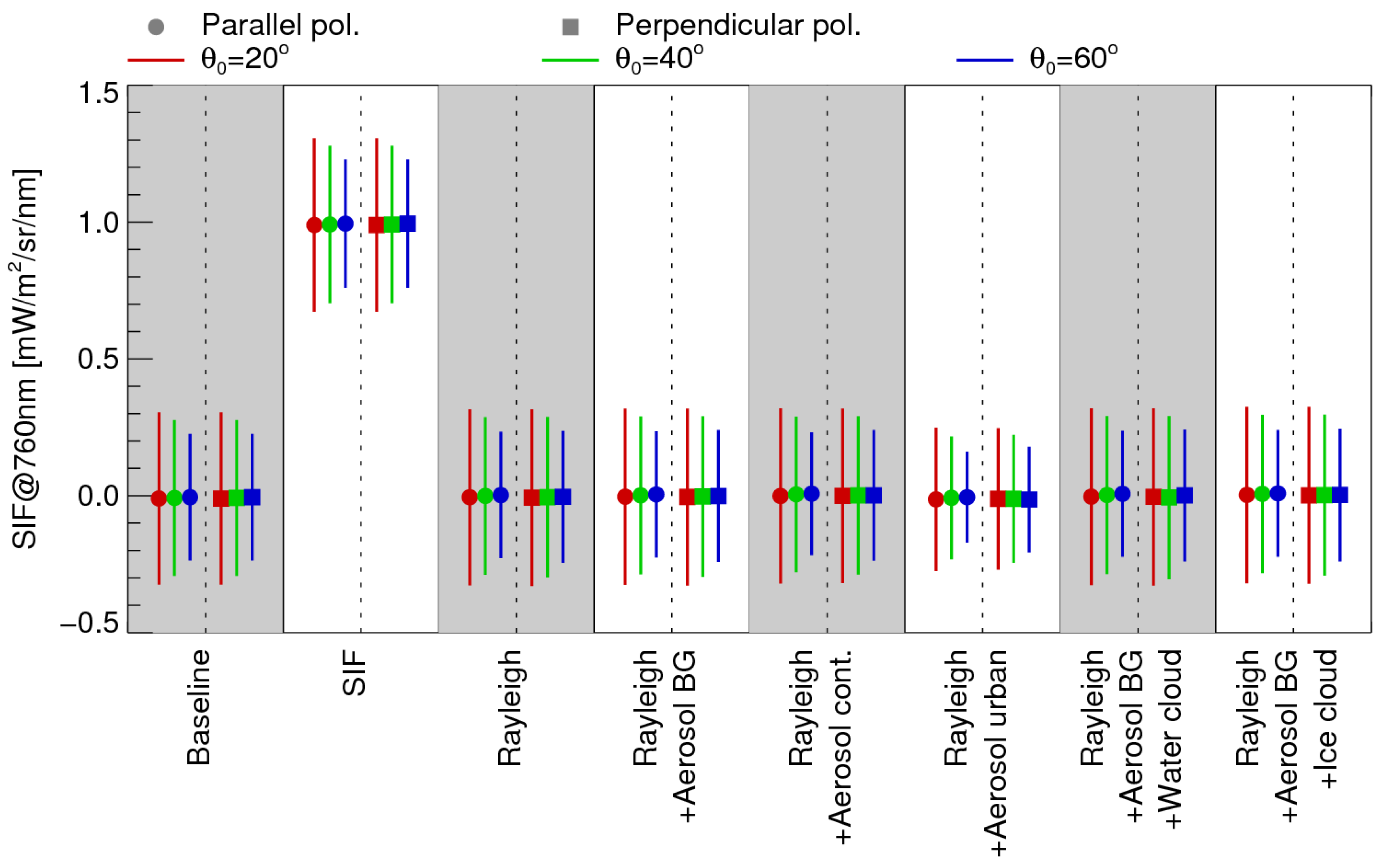
Each scenario is analyzed for three solar zenith angles (20°, 40°, and 60°) and for two directions of polarization (parallel and perpendicular to the SPP). The satellite zenith angle is set to 0° (nadir).
The SIF scenario adds 1 mW/m/sr/nm chlorophyll fluorescence at 760 nm to the simulated measurement of the baseline scenario. The XCO+6 ppm scenario has an increased CO concentration of 15 ppm, 10 ppm, and 5 ppm in the three lowermost layers, so that the column-average concentration is enhanced by 6 ppm.
All scattering related scenarios are more complex for the retrieval because of FOCAL’s scattering approximations. The Rayleigh scenario adds Rayleigh scattering to the baseline scenario; the Rayleigh optical thickness at 760 nm for this scenario is about 0.026. Rayleigh+Aerosol BG additionally includes a (primarily) stratospheric background aerosol with an AOT (aerosol optical thickness at 760 nm) of 0.019 (0.003 at 1600 nm and 0.001 at 2050 nm). Rayleigh+Aerosol cont adds a continental aerosol to the boundary layer so that the total AOT becomes 0.158 (0.060 at 1600 nm and 0.037 at 2050 nm). Rayleigh+Aerosol urban adds a strong contamination with urban aerosol to the boundary layer and the total AOT becomes 0.702 (0.245 at 1600 nm and 0.151 at 2050 nm).
The scenarios Rayleigh+Dark surface, Rayleigh+Bright surface, and Rayleigh+Ocean glint distinguish from the Rayleigh scenario only by their surface reflection properties. Rayleigh+Dark surface and Rayleigh+Bright surface correspond to the Rayleigh scenario but with an albedo multiplied with 0.7 and 1.4, respectively. The Rayleigh+Ocean glint scenario deviates from the assumption of a Lambertian surface bidirectional reflectance distribution function (BRDF); it includes an ocean surface at a wind speed of 5 m/s, 37° to the solar principal plane (SPP). Additionally, the satellite zenith angle of this scenario is set to 0.75 times the solar zenith angle so that the satellite looks near the glint spot of specular reflectance.
Two cloud scenarios (Rayleigh+Aerosol BG+Water cloud and Rayleigh+Aerosol BG+Ice cloud) add a sub-visible water or ice cloud to the Rayleigh+Aerosol BG scenario. The water cloud has a height of 3 km, droplets with an effective radius of 12 µm, and a COT (cloud optical thickness at 500 nm) of 0.039. The ice cloud is made of fractal particles with an effective radius of 50 µm, has a height of 8 km, and a COT of 0.033.
Appendix B lists important input parameters which have been used to perform the SCIATRAN RT calculations for all scenarios.
3.2.3. Results
Primarily, we are interested in XCO
retrieval results of high quality; the correct retrieval of other state vector elements is less important as long as the XCO
quality is not affected.
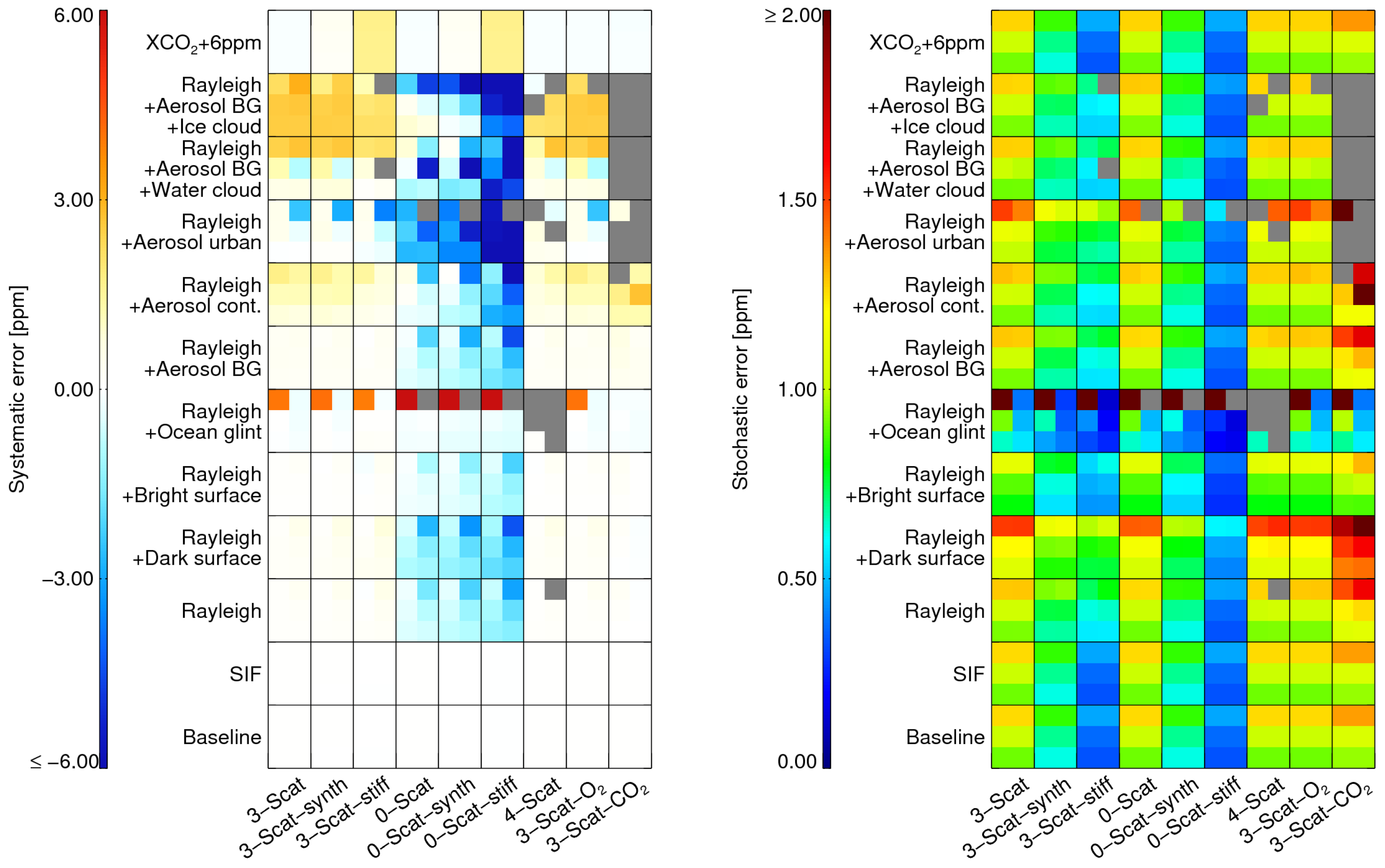
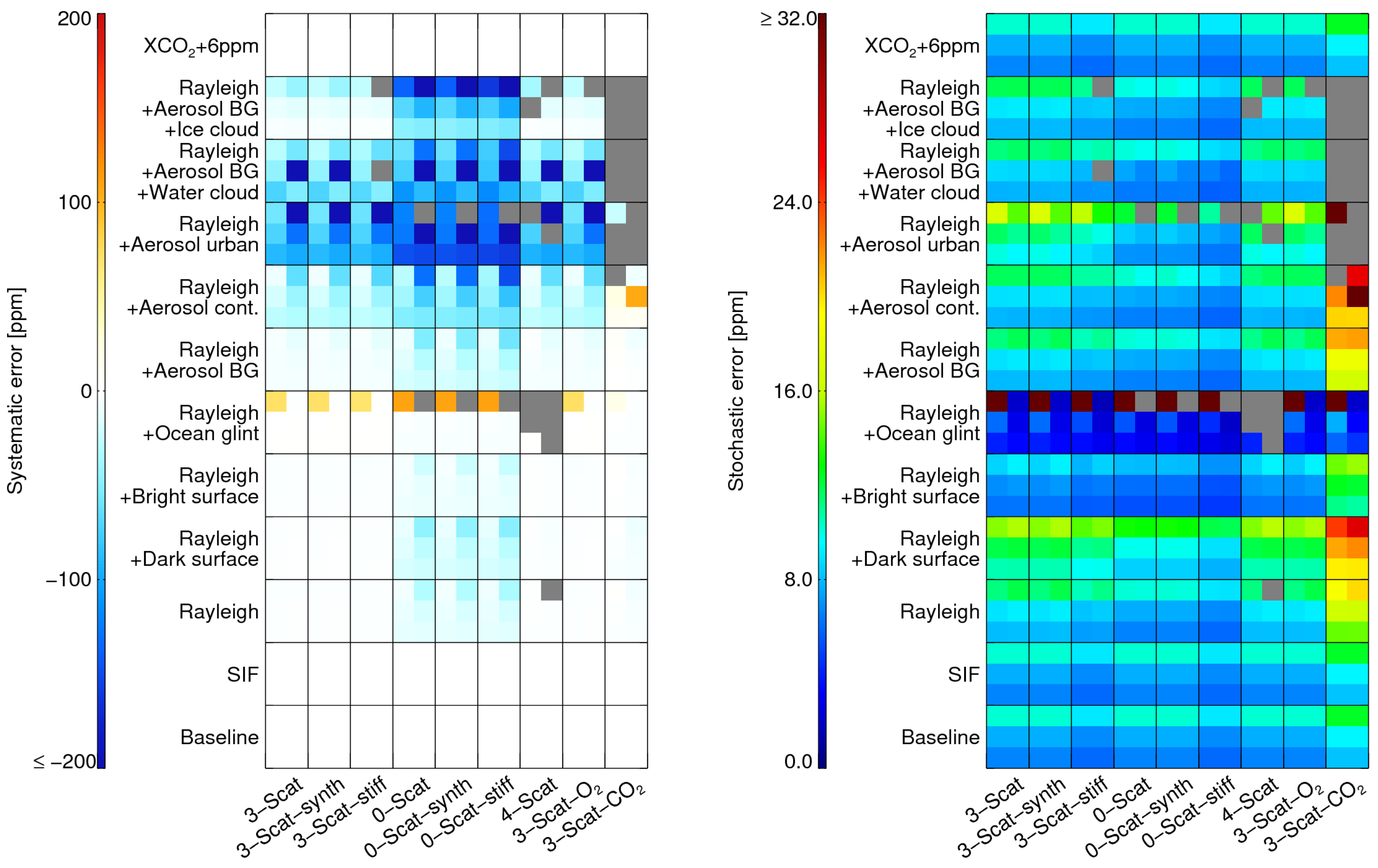
Figure 7 summarizes the systematic errors and stochastic uncertainties of the retrieved XCO
for all retrieval setups and geophysical scenarios.
The baseline scenario is mainly to ensure consistency of the RT used to simulate the measurements (SCIATRAN) and the RT of the retrieval (FOCAL). Additionally, the baseline scenario allows estimates of the retrieval’s noise error. With SCIATRAN, it is not simply possible to simulate FOCAL’s scattering approximations, that is why this scenario excludes scattering. The systematic errors of the baseline scenario are always very small (0.03 ppm at maximum), which confirms the RT consistency in the absorption only case and ensures that, e.g., the number of particles is basically identical in the SCIATRAN and the FOCAL “world”.
The systematic errors of the SIF scenario are not larger than for the baseline scenario, because i) SIF is solely determined from the SIF fit window and ii) there is no SIF flux emitted in the CO fit windows.
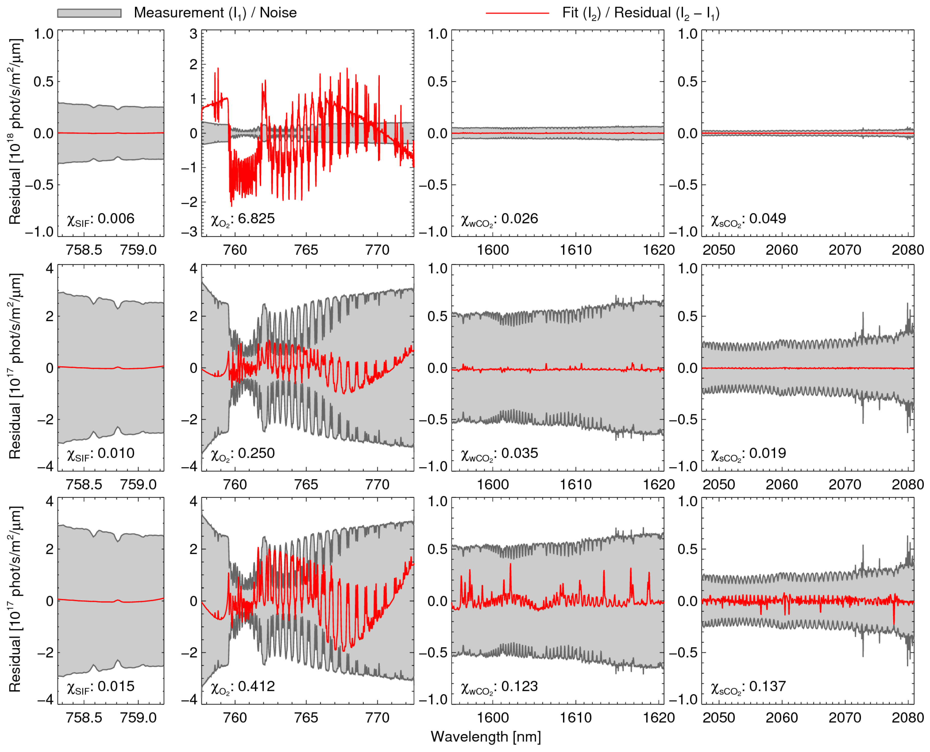
A more complex case for FOCAL is the
Rayleigh scenario, because Rayleigh scattering takes place in the entire atmospheric column with a peanut-shaped SPF. This means, it cannot be expected that FOCAL is able to perfectly fit the simulated measurement.
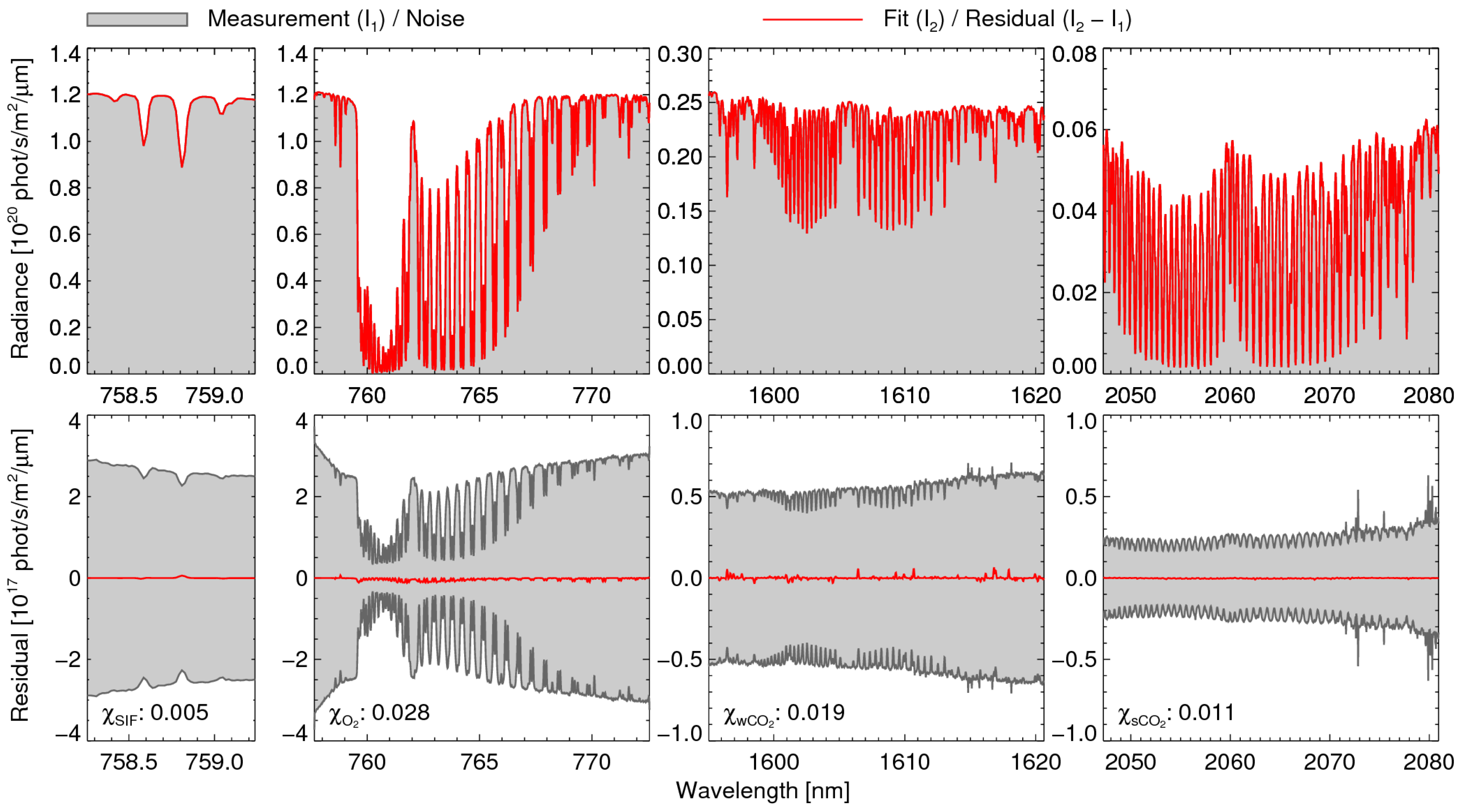
Figure 8 (top) shows a spectral fit in all fit windows but with a state vector not including any scattering parameter, so that the geophysical results (e.g., XCO
) become identical with those of the
0-Scat setup.
Not surprisingly, the residual in the O
fit window becomes large compared to the simulated measurement noise (
). The residuals in the CO
fit windows are already small compared to the instrumental noise even without fitting scattering parameters (
,
). This is only partly explained by Rayleigh scattering having an Ångström exponent of four and, therefore, a much smaller scattering optical thickness at longer wavelengths. It also indicates that disentangling scattering parameters and CO
concentration from measurements in the CO
fit windows may be difficult. In other words, most of the scattering information must be imprinted in the residual of the O
fit window. This is also why the results of the
3-Scat-O setup are similar to the
3-Scat setup and why the
3-Scat-CO retrievals are often not converging (
Figure 7).
Allowing the
3-Scat retrieval setup to fit the scattering parameters
,
, and
Å, reduces the O
residual to become typically four times smaller than expected from instrumental noise (
,
Figure 8, middle). Simultaneously, the XCO
error reduces from −0.43 ppm to 0.10 ppm (−0.89 ppm and 0.16 ppm for perpendicular polarization).
All other scattering related scenarios are even more “complicated” for FOCAL because different particles contribute to scattering. For example, cloud particles have different properties like height or Ångström exponent as aerosol particles, but FOCAL can only retrieve one effective height and one effective Ångström exponent. Additionally, the SPFs of aerosols and clouds are less isotropic. Therefore, the residuals (
Figure 8, bottom) and more importantly, the systematic errors typically increase for these scenarios (
Figure 7, left).
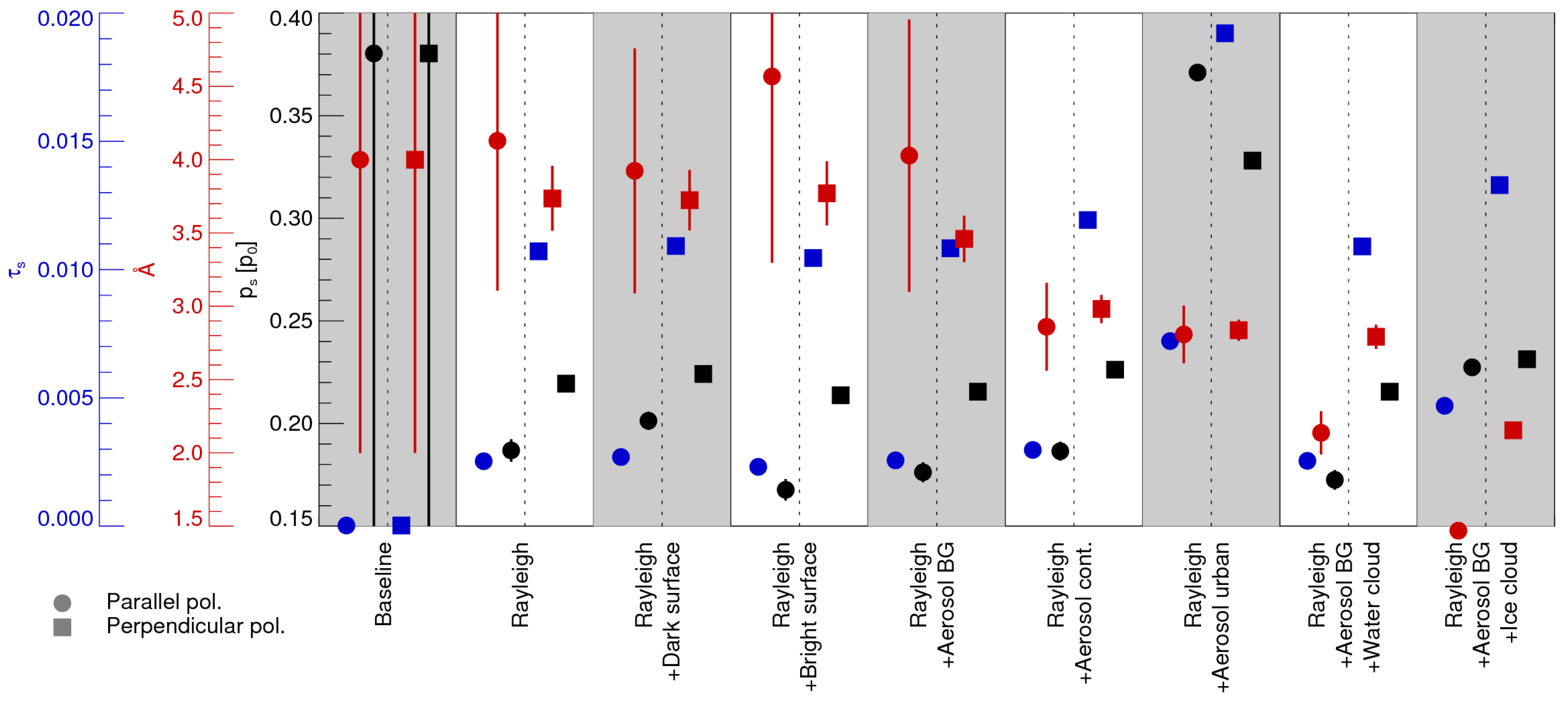
Figure 9 shows the retrieved scattering parameters for the
3-Scat setup and a set of scattering related plus the baseline scenario. As the baseline scenario does not include any scattering, the retrieved
and
Å are close to their a prior values and have a large a posteriori uncertainty. Consistent with the expectations, the retrieved effective Ångström exponent is close to four (about 3.8) for the Rayleigh scenario and reduces to 2.8–3.6 for the aerosol and 2.1–2.6 for cloud scenarios. This means the scattering optical thickness at longer wavelengths increases relative to the shorter wavelengths. Rayleigh scattered light is unpolarized in forward and backward scattering direction but polarized perpendicular to the incident beam for scattering angles of 90°. For this reason, the retrieved
is always larger for the polarization direction perpendicular to the SPP. As expected, this effect is more/less pronounced for larger/smaller solar zenith angles (not shown). In contrast to the
3-Scat and
4-Scat setups, the
0-Scat retrievals cannot fit
which results in a larger polarization dependency of the resulting systematic errors (
Figure 7, left).
As shown in
Figure 9, the highest scattering optical thicknesses at 760 nm are obtained for the urban aerosol and the cloud scenarios. However, the quantitative interpretation of the retrieved values of
and
is difficult because they are effective values representing all kinds of scattering in the atmospheric column. Additionally,
and
may not be perfectly independent because light path modifications are expected to become larger when enhancing the height of the scattering layer. It can be observed that the retrieved values of
are generally smaller than the scattering optical thicknesses computed by SCIATRAN (
Section 3.2.2). This is expected because of the different SPFs assumed by SCIATRAN and FOCAL. Especially for Mie scattering of cloud and aerosol particles, the SCIATRAN simulations use SPFs with a distinct forward peak contributing to the total scattering optical thickness. FOCAL, however, interprets scattering in forward direction as transmission (not contributing to
). This means,
is best comparable for the
Rayleigh scenario with a SPF without forward peak.
The scenarios Rayleigh, Rayleigh+Dark surface, and Rayleigh+Bright surface differ by their surface albedo. However, the retrieved scattering parameters show little differences because in FOCAL these parameters represent (within the limits of the made assumptions) approximations of real geophysical quantities.
Applying FOCAL to the
Rayleigh+Ocean glint scenario with a highly non-Lambertian surface BRDF results in systematic XCO
and XH
O errors usually comparable to the
Rayleigh scenario (
Figure 7 and
Figure 10, left) except for solar zenith angles of 60° and polarization parallel to the SPP. In near-glint geometry, specular reflectance dominates the radiation field but with increasing solar zenith angle the reflected radiation becomes more and more polarized. As a result the direct photon path often dominates (if not observing parallel polarization at large solar zenith angles) and an imperfect parameterization of scattering becomes less important. The domination of the direct photon path also results in a larger total radiance and, correspondingly, smaller stochastic errors in perpendicular polarization (
Figure 7 and
Figure 10, right). The larger systematic XCO
errors of about 4 ppm at 60° and parallel polarization are a result of the poor surface reflectivity in this observation geometry and associated with large stochastic errors of about 8 ppm and little error reduction (analog for XH
O). This means, applied to real measurements, such retrievals would most certainly be filtered during post processing. Note that due to the non-Lambertian surface, the retrieved albedo may have values larger than one.
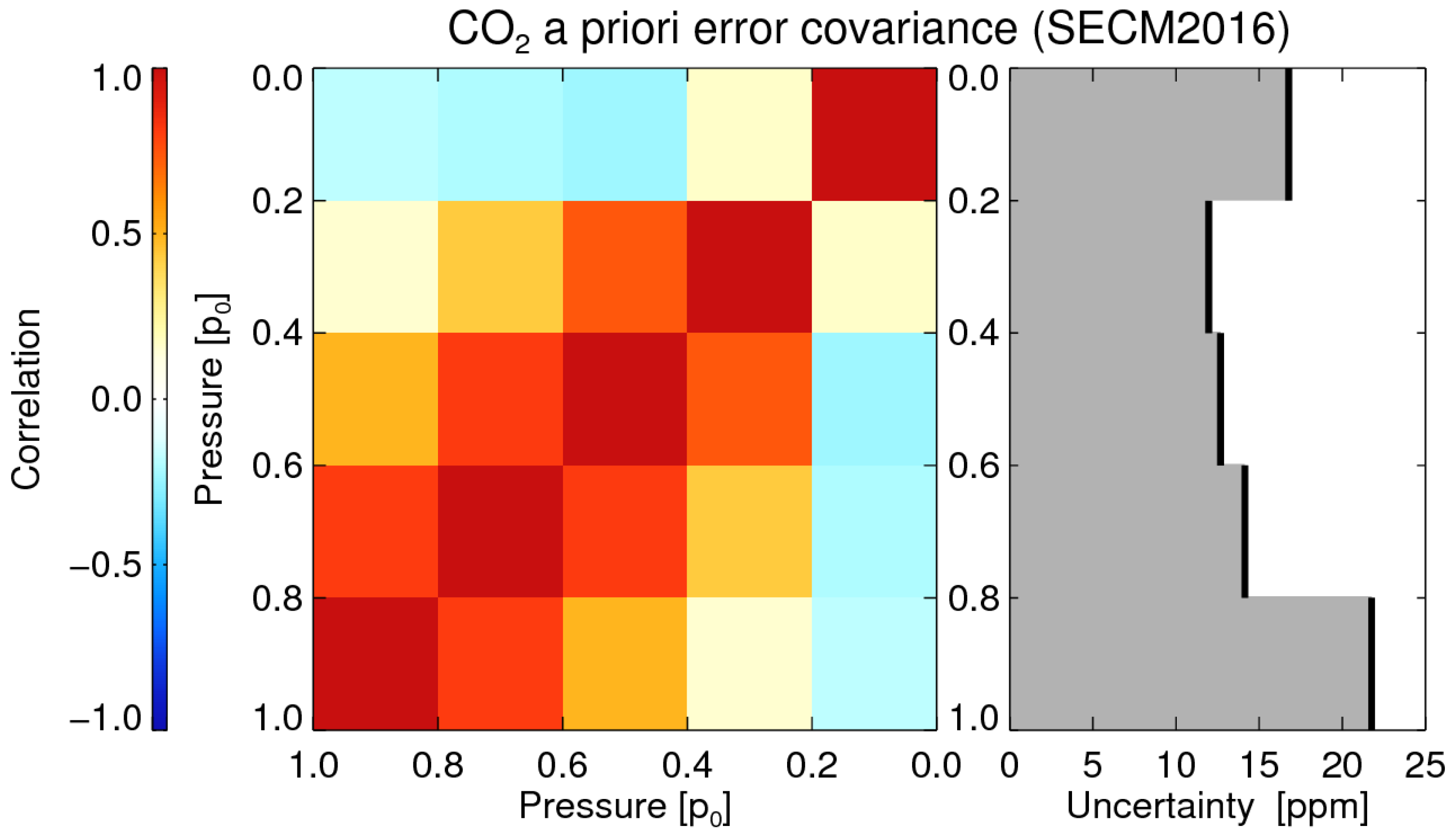
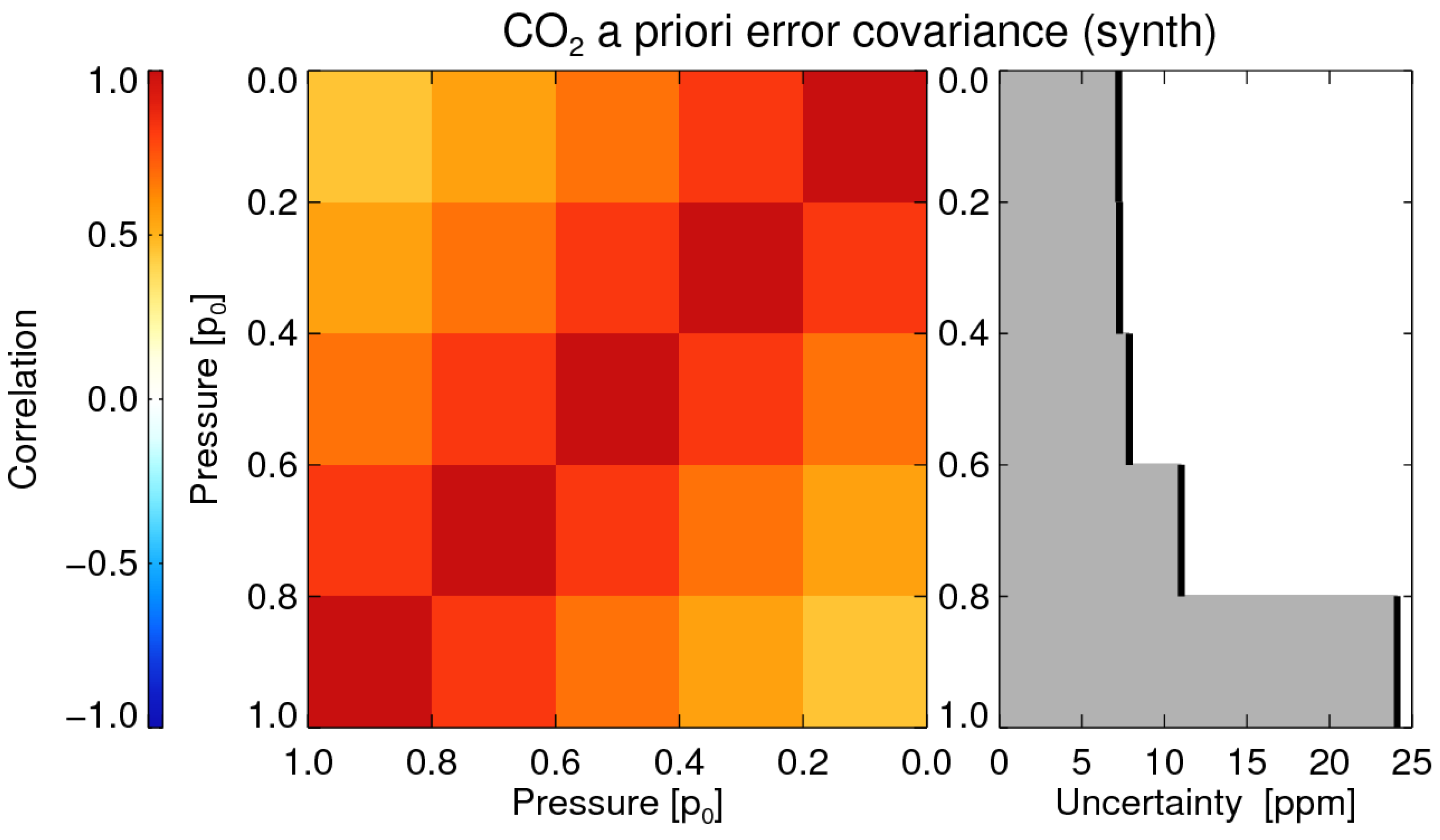
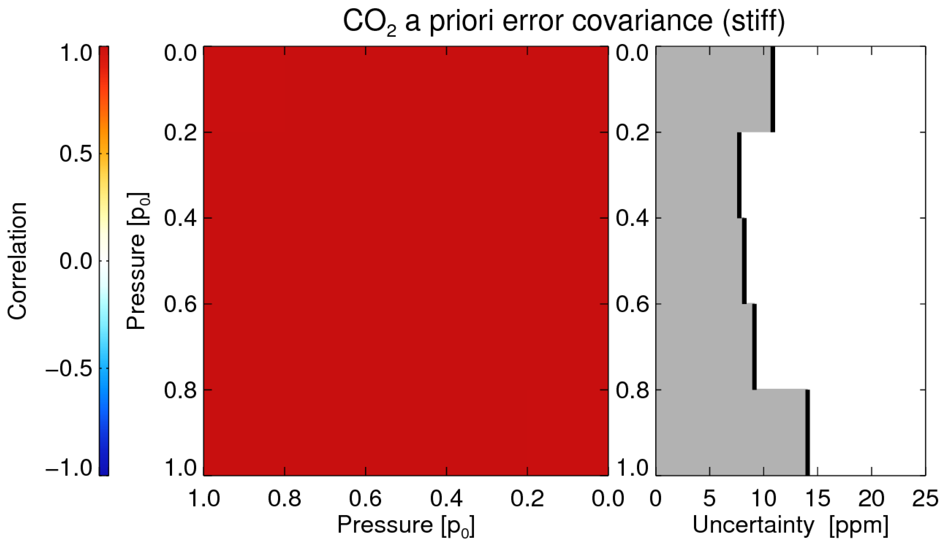
Figure 7 (right) shows that the shape of the CO
a priori error covariance matrix can considerably influence the stochastic XCO
a posteriori uncertainty, even though the a priori XCO
uncertainty has not been changed. Stiffening the covariance matrix by enhancing the layer-to-layer correlations as done for the
synth and
stiff setups (
Figure 11 and
Figure 12), reduces the stochastic XCO
uncertainty from typically about 1 ppm to 0.7 ppm (
synth) and 0.4 ppm to 0.6 ppm (
stiff), which does not necessarily mean that results actually improve.
Except for the
XCO+6 ppm scenario, the systematic errors of the
3-Scat,
3-Scat-synth, and
3-Scat-stiff setups are very similar. This is not the case for the
0-Scat,
0-Scat-synth, and
0-Scat-stiff setups for which the systematic errors increase with stiffness of the CO
a priori error covariance matrix. Apparently, the (loose) profile retrieval of the
0-Scat scenario happens to somewhat compensate light path related errors. In the case of the
3-Scat setups, the scattering parameters are doing this job.
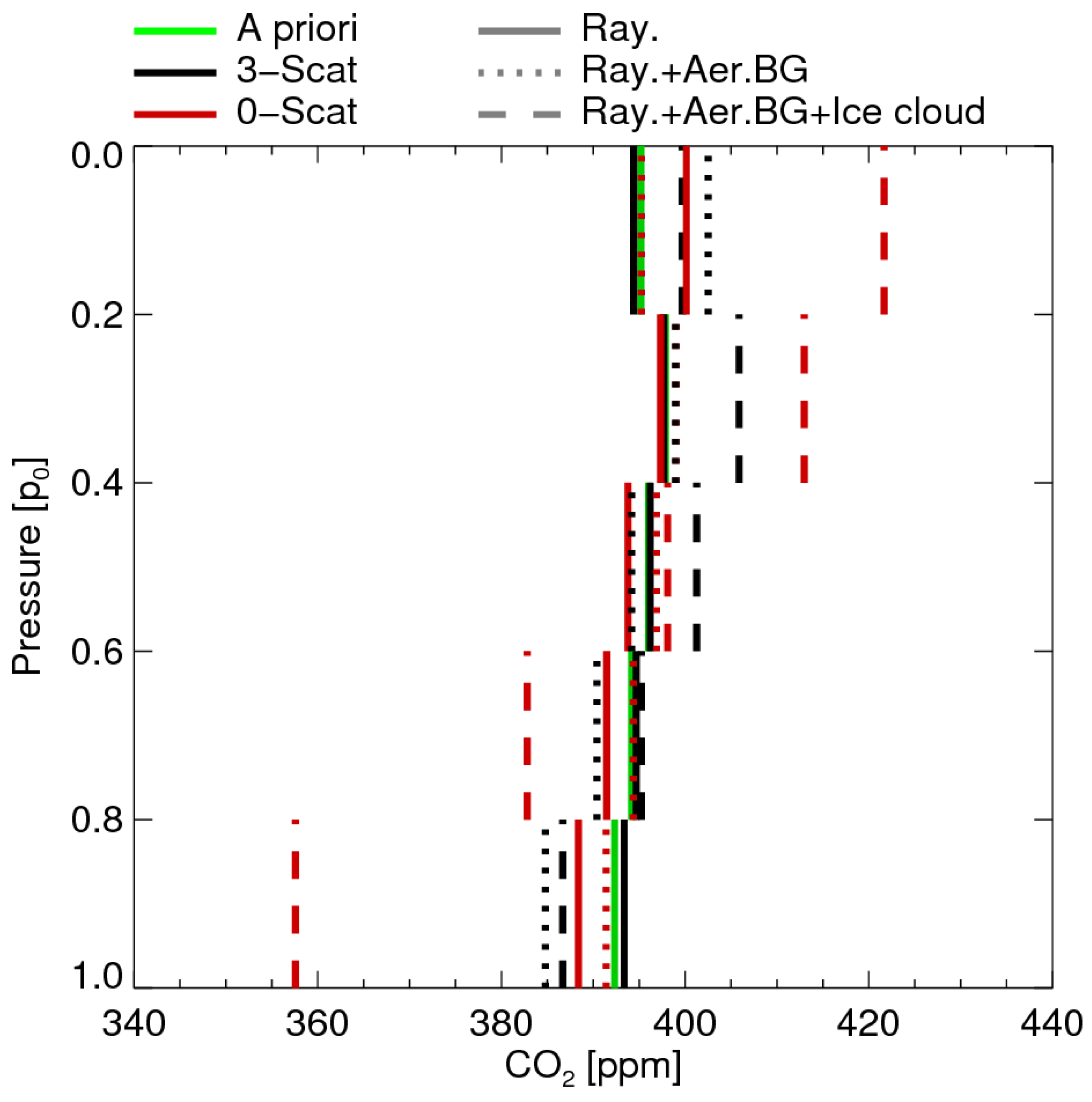
Figure 13 shows, that the largest deviations of the retrieved profiles from the true profile (a priori) indeed occur for the
0-Scat setup.
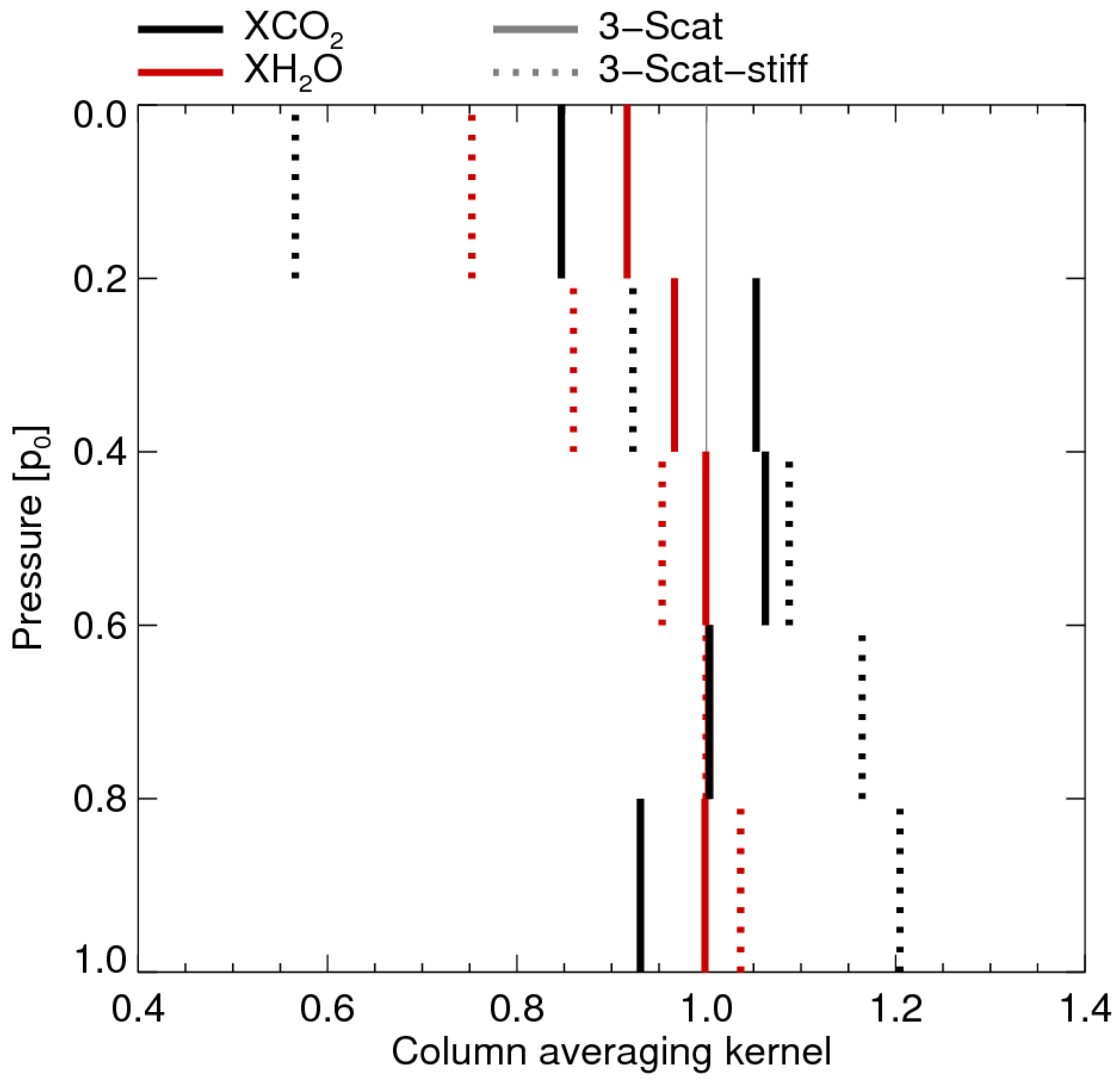
The degree of freedom for the CO
profile is about 2.2 for the
3-Scat setup and reduces to 1.8 for the
3-Scat-synth and 1.0 for the
3-Scat-stiff setup. The degree of freedom for the H
O profile reduces from 2.2 for the
3-Scat setup to 1.0 for the
3-Scat-stiff setup. Additionally, the column averaging kernels (AKs) change and show larger deviations from unity; specifically, as illustrated in
Figure 14, the XCO
AK increases to about 1.2 in the boundary layer and reduces to 0.6 in the stratosphere. As a result, the systematic error (in this particular case, the smoothing error) increases for the
stiff setups to about 1.6 ppm (
Figure 7, left).
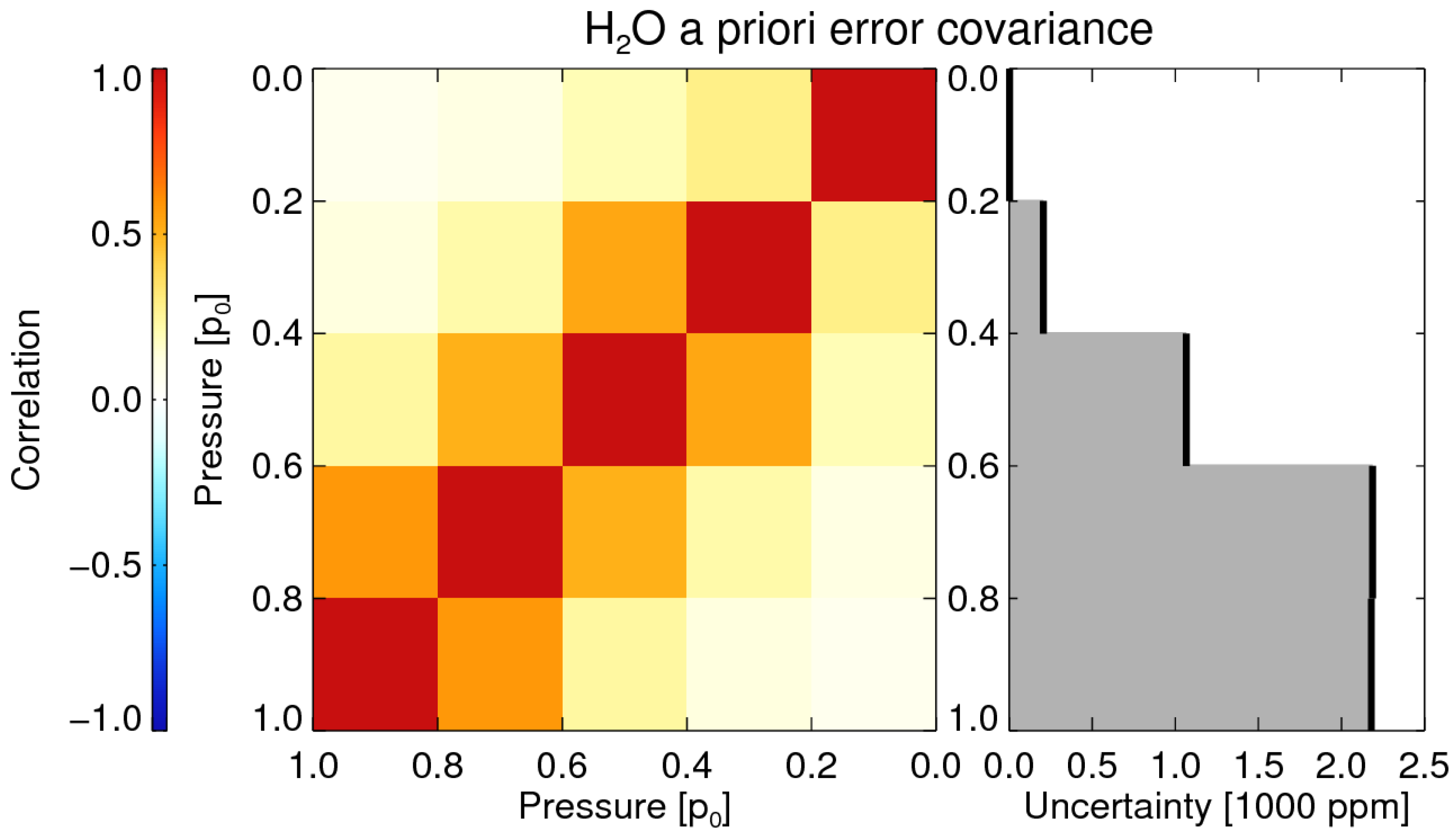
As illustrated in
Figure 10, scattering related systematic XH
O errors are usually negative and larger for the
0-Scat setups. Stiffening the H
O a priori error covariance matrix has little influence on the systematic or stochastic error which is usually about 10 ppm. SIF is almost not influenced by the mostly low scattering optical thicknesses of the tested scenarios and the stochastic a posteriori error is usually between 0.2 and 0.3 mW/m
/sr/nm (
Figure 15).
All tested retrieval setups do not have the ability to change the number of dry-air particles in the atmospheric column, e.g., by fitting the surface pressure, or a shift of the temperature profile. As a result, relative errors of the number of dry-air particles computed from the meteorological profiles directly translate into relative errors of the retrieved XCO and XHO. For example, a 1 hPa error of the surface pressure will result in a XCO error of about 0.4 ppm.

 ,
, 
