Multi-Scale Evaluation of the SMAP Product Using Sparse In-Situ Network over a High Mountainous Watershed, Northwest China

Abstract

As the latest L-band mission to date, evaluation of the Soil Moisture Active Passive (SMAP) products is one of its post-launch objectives. However, almost all previous studies have been conducted at the core validation sites (CVS) of the SMAP mission. This paper presents an evaluation of the SMAP soil moisture Level 3 (L3) and Level 4 (L4) products under different vegetation types at multiple tempo-spatial scales over the upper reach of the Heihe River Watershed, a topographically complex mountainous area in Northwest China. This was done through comparisons of the L3 and L4 products with ground-based observations from a sparse in situ network of permanent and temporary stations from 1 April 2015 to 22 June 2017. Results show that, compared with in situ observations at point scale, both the L3 and L4 products represent the temporal trends of the in situ observations in the study area well, with R values of 0.601 and 0.538 for the L3 ascending and descending products, respectively, and ranging from 0.353 to 0.410 for the L4 product at eight overpassing moments. However, because of the uncertainties of brightness temperature T_Bp and effective temperature T_eff as well as their propagations in the inversion algorithm, both products did not achieve the accuracy of 0.04 m³/m³ in mountainous area. These uncertainties also result in the “dry bias” of the SMAP products in almost all the evaluations to date. Compared with areal average values at the watershed scale, the L3 product is far beyond the accuracy of 0.04 m³/m³ and the L4 product basically achieves the accuracy. In vegetation-covered land, the suitability and the variability of the coefficient b_p result in both products performing best in cropland, then coniferous forest, sparse grassland, dense grassland, and alpine meadow, and worst in shrub. In barren land, the errors in estimating surface roughness h caused by the complex topography lead to poor performance of the SMAP products. With the relative errors of the SMAP brightness temperature observations and the corresponding land model forecast in the assimilation; the L3 and L4 products show different performance at both temporal and spatial scales; and the L3 product provides more reliable soil moisture estimates in the study area. Based on the results of this study, we propose: quantifying the uncertainties in estimating brightness temperature T_Bp and effective temperature T_eff; determine coefficient b_p and surface roughness h factor under various conditions; improving Goddard Earth Observing Model System Version 5 (GEOS-5) model; and deriving the SMAP-only climatology to improve the SMAP soil moisture estimates in the future.

1. Introduction

Soil moisture is a key variable in the global energy and water cycle, and is also important in many land surface disciplines such as agriculture, hydrology and environmental sciences [1,2]. In recent years, it has been considered as an Essential Climate Variable (ECV) by the World Meteorological Organization [3]. Although in situ measurements have been considered as the most accurate methods for obtaining soil moisture at point scale, it is impossible to represent the spatial distribution of highly variant soil moisture at large scale from in situ measurement networks [4,5]. In recent decades, satellite products of soil moisture at large scale have become available via different active and passive microwave remote sensing techniques [6,7,8,9,10]. Compared with C-band and X-band products, L-band products are much more suitable for the estimation of soil moisture because of their higher soil penetration depth, higher frequency and better vegetation penetration [11], especially for regions where soil moisture is a controlling factor on land-atmosphere exchanges [9].

Employing both an L-band radar and an L-band radiometer, the National Aeronautics and Space Administrati (NASA) Soil Moisture Active Passive (SMAP) satellite mission was launched on 31 January 2015. Both radar and radiometer instruments shared a rotating 6-m mesh reflector antenna on a platform in a 685-km sunsynchronous near-polar orbit, viewing the Earth’s surface at a constant incidence angle of 40° with swath width of 1000 km [12]. However, the radar instrument encountered an irrecoverable hardware failure on 7 July 2015, and the production of soil moisture data products continues using the radiometer data alone [12,13]. The SMAP mission delivers data products of four levels, including the instrument measurements (Level 1), geophysical retrievals (swath based, Level 2, and daily composite, Level 3), and land surface models assimilating SMAP measurements (Level 4) [12,14]. The SMAP mission aims to provide soil moisture estimates in the top 5 cm of soil over the global land area with an unbiased root mean square error (ubRMSE) less than 0.04 m³/m³ [14,15]. To meet the science requirements, one of its post-launch objectives is to validate the accuracy of the science data products [14]. However, so far, only a few validations of the SMAP products have been conducted, and almost all of them have been carried out at the core validation sites (CVS) [12,16,17,18,19,20,21,22]. Because observations from the CVS have been used to refine and validate retrieval algorithms, it is important to validate the SMAP products over other regions beyond the CVS [12,14,21,23].

The objectives of this work are first to validate the SMAP soil moisture Level 3 and Level 4 products under different vegetation types at multiple tempo-spatial scales over the upper reach of the Heihe River Watershed, a topographically complex, high mountainous area in Northwest China, then to quantify the differences between both products, and subsequently determine their suitability in mountainous areas. These were done through comparisons with ground-based measurements from a sparse in situ network of permanent and temporary stations from 1 April 2015 to 22 June 2017. Finally, the suitability of both products is analyzed and the future improvements are suggested.

2. Study Area and Datasets

2.1. Study Area

The Heihe River, with a drainage area of 128,000 km², is the second largest inland river (or terminal lake) in China [24]. The upper reach of the Heihe River Watershed is located in the Qilian Mountain ranges (Figure 1), with a length of 313 km and a drainage area of 10,009 km², producing the majority of runoff for the entire Heihe River Watershed [25]. The local climate is influenced by both the continental climate and the Qinghai-Tibet plateau climate [26], the mean annual temperature ranges from −3.1 to 3.6 °C with the minimum temperature of −28 °C. Mean annual precipitation ranges from 250 mm below 1900 m asl (meters above sea level) to 700 mm above 3600 m asl, and most precipitation (over 60%) falls between June and September. The elevation in the region ranges from 1674 to 5584 m asl [25,27].

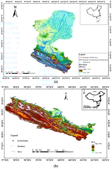
Figure 1. The Study area (a) The Heihe River Watershed in Northwest China; (b) The upper reach of the Hehe River Watershed.

In the upper reach of the Heihe River Watershed, the major vegetation types include coniferous forest (Picea crassifolia), shrub (Potentilla fruticosa), steppe (Stipa purpurea Griseb), alpine meadow (Kobresia pygmaea Clarke), alpine sparse vegetation (Saussurea medusa Maxim), and desert (Sympegma regelii Bunge) [28]. There are various soil types in the study area, e.g., aeolian sandy soil, cold desert soil, alpine meadow soil, mountain swamp chestnut soil and mountain marshy soil [26]. Because of the complex terrain surface, it is difficult to accurately estimate soil moisture at watershed scale in the study area [29].

2.2. The SMAP Product

The NASA’s SMAP satellite mission, was designed to provide global mapping of soil moisture and landscape freeze/thaw state with high resolution [9]. It aims to provide soil moisture estimates in the top 5 cm of soil over the global land area, excluding surfaces with permanent ice and snow, urban areas, wetlands, and vegetated areas with vegetation water content greater than 5 kg/m² [14]. The mission requirement is ubRMSE less than 0.04 m³/m³ for the surface soil moisture for the 36 km and 9 km gridded products within the retrieval domain.

The SMAP L3_SM_P_E and L4_SM_gph products from 1 April 2015 to 22 July 2017 over the study area are selected for validation in this research. Given the failure of the SMAP radar in July 2015 and the short measurement period, the L3_SM_P_E product (hereinafter referred to as “the L3 product”) is daily geophysical retrieval at 9 km by 9 km of half orbits based on the downscaling results of the observed brightness temperature with a resolution of 36 km by 36 km. The L4_SM_gph product (hereinafter referred to as “the L4 product”) is modeling value-added surface soil moisture product at a 3-h interval based on the SMAP retrievals and simulations by Goddard Earth Observing Model System Version 5 (GEOS-5) [14]. Both the SMAP L3 and L4 products are available with equally spaced grid at ~9 km by 9 km, known as the Discrete Global Grid (DGG) [30]. The entire study area is covered by roughly 410 DGGs of the SMAP products. Both products have been distributed by NASA National Snow and Ice Data Center Distributed Active Archive Center (NSIDC DAAC) and the NASA Alaska Satellite Facility Distributed Active Archive Center (ASF DAAC). Data and further details are available at http://nsidc.org/.

2.3. Sparse In situ Network

Sparse network measurements can be used as additional resources to expand the spatial and temporal scopes of the validation [12,23]. In this study, the sparse in situ soil moisture network was established in June 2013 by authors’ team over the upper reach of the Heihe River Watershed. It includes 35 nodes, which were established based on the combinations of vegetation and soil types in the study area (Figure 1, Table 1). Although with only 35 nodes, the sparse in situ network provides observations on the main characteristics of vegetation-soil types, making it representative to compare with the dense in-situ networks [31].

Table 1. The in-situ observation points in the study area.

Station	Longitude	Latitude	Altitude (m asl)	Vegetation	Sand (%)	Silt (%)	Clay (%)	Soil Types
D1	99.758	38.910	2151	Sparse grassland	33.890	58.970	7.140	Typical Sierozems
D2	99.520	38.781	2556	Sparse grassland	32.330	60.020	7.650	Light Castanozems
D3	99.988	38.955	1827	Sparse grassland	38.030	55.880	6.090	Clay gray desert soils
D4	100.013	38.455	2370	Sparse grassland	27.819	65.997	6.184	Typical Castanozems
D5	101.350	38.095	2558	Dense grassland	57.845	37.866	4.289	Light Castanozems
D6	99.186	39.146	2604	Sparse grassland	25.207	66.891	7.902	Light Castanozems
D7	98.329	38.899	3317	Sparse grassland	22.072	69.032	8.896	Calcareous Frigid frozen soils
D8	98.805	39.323	2170	Sparse grassland	20.128	72.581	7.291	Saturated Frigid frozen felt soils
D9	99.232	38.724	3622	Dense grassland	34.464	58.182	7.354	Saturated Frigid frozen felt soils
D10	97.824	39.338	3117	Sparse grassland	9.774	82.888	7.337	Calcareous Frigid frozen soils
D11	100.220	38.560	2890	Coniferous forest	11.134	81.961	6.905	Typical Castanozems
D12	99.711	38.789	2498	Coniferous forest	19.863	73.599	6.538	Typical Grey-cinnamon soils
D13	101.048	38.189	2977	Shrub	13.816	78.380	7.804	Peat Frigid felt soils
D14	100.418	38.480	2676	Coniferous forest	44.335	50.187	5.478	Light Castanozems
D15	101.050	38.160	3146	Shrub	9.022	83.357	7.621	Peat Frigid felt soils
D16	100.616	38.031	3105	Dense grassland	28.634	65.963	5.403	Saturated Frigid frozen felt soils
D17	100.929	38.065	3300	Sparse grassland	25.191	67.730	7.079	Typical Chernozems
D18	101.378	38.125	2787	Dense grassland	27.410	65.161	7.429	Dry farming Chernozems
D19	100.908	38.274	2697	Cropland	14.628	78.103	7.268	Typical Castanozems
D20	99.670	39.119	2147	Barren land	20.753	71.602	7.644	Calcareous Frigid calcic soils
D21	97.866	39.633	2770	Sparse grassland	25.212	68.056	6.732	Calcareous Frigid calcic soils
D22	97.971	39.535	2303	Sparse grassland	27.226	66.467	6.307	Saturated Frigid frozen felt soils
D23	98.351	39.472	2390	Sparse grassland	41.253	53.508	5.239	Typical Frigid frozen calcic soils
D24	98.756	38.788	4109	Barren land	41.699	52.654	5.648	Typical Frigid desert soils
D25	99.475	38.611	4155	Barren land	54.860	40.260	4.880	Saturated Frigid frozen felt soils
D26	100.237	38.184	3252	Sparse grassland	29.832	61.556	8.612	Typical Castanozems
D27	100.147	38.585	2465	Dense grassland	8.744	81.255	10.002	Light Castanozems
D28	101.269	38.299	2601	Dense grassland	14.337	73.138	12.524	Typical Castanozems
D29	99.623	38.409	3249	Dense grassland	22.241	69.842	7.917	Peat Frigid felt soils
D30	101.050	38.165	3109	Dense grassland	20.356	73.725	5.920	Saturated Frigid frozen felt soils
D31	99.969	38.241	2920	Dense grassland	24.748	69.119	6.133	Saturated Frigid frozen felt soils
D32	99.485	38.592	3800	Alpine meadow	26.737	63.807	9.455	Typical Gray calcic soils
D33	100.286	38.554	2698	Dense grassland	19.860	73.600	6.540	Typical Castanozems
D34	100.937	38.215	2886	Dense grassland	9.480	84.390	6.130	Typical Chernozems
D35	99.915	38.833	2839	Dense grassland	27.930	67.160	4.910	Typical Castanozems

Through experimental analysis, soil textures of the in situ nodes are silt loam, silt, and sandy loam according to the United States Department of Agriculture (USDA) soil classification system, with the silt loam being the dominant texture (Table 1). For each node, soil moisture at depths of 5, 15, 25, 40 and 60 cm was measured at 30-min intervals by soil moisture sensor (Decagon’s 5TE), and the data at depths of 5 cm were used as the surface soil moisture data in this study. The measurements by the soil moisture sensor were calibrated using field collected soil samples [32,33]. Soil samples were first weighed in the field and then weighed again after oven dried for 24 h at 105 °C. The details of the field sampling and analysis can be found in [33,34]. According to the manual provided by Decagon Company [35], the soil moisture at each in situ point was subsequently calculated based on the weight difference between the wet and dry soil and volume of the container.

3. Methods

3.1. Evaluation Metrics

Both the SMAP L3 and L4 products, as well as the in situ observations are in units of m³/m³. In order to facilitate comparisons with other evaluation studies, we used the following three metrics for the validation in this study. The formula of three statistical indicators, correlation coefficient (R), root-mean-square errors (RMSE) and the mean bias (bias) are as follows [5,9,36,37].

$$R=\frac{{\displaystyle {\sum }_{t=1}^n(S{M}_t^{obs}-{\overline{SM}}^{obs})(S{M}_t^{sat}-{\overline{SM}}^{sat})}}{\sqrt{{\displaystyle {\sum }_{t=1}^n{(S{M}_t^{obs}-{\overline{SM}}^{obs})}^2}}\sqrt{{\displaystyle {\sum }_{t=1}^n{(S{M}_t^{sat}-{\overline{SM}}^{sat})}^2}}}$$

(1)

$$RMSE=\sqrt{\frac{{\displaystyle {\sum }_{t=1}^n{(S{M}_t^{obs}-S{M}_t^{sat})}^2}}{n}}$$

(2)

$$\mathrm{bias}={\overline{SM}}^{sat}-{\overline{SM}}^{obs}$$

(3)

where, $S{M}_t^{obs}$ and $S{M}_t^{sat}$ are the soil moisture values of ground sites and satellite-based products on tth day, ${\overline{SM}}^{obs}$ and ${\overline{SM}}^{sat}$ are the average values of ground sites and satellite-based products during the evaluation period, n is the number of days. As the target accuracy of the SMAP product is expressed by ubRMSE (unbiased RMSE) [14,15], ubRMSE has also been analyzed in this study. It is related to RMSE through ${RMSE}^2{=ubRMSE}^2+bia{s}^2$.

3.2. Temporal Stability Analysis

The temporal stability analysis has been conducted to compare the similarity of the spatial distributions of soil moisture data between the L3 and L4 products, over the same period from 1 April 2015 to 22 June 2017 [11,38,39,40]. For each grid x, the stability of soil moisture estimates from one time step to another is evaluated by mean relative difference (MRD) ${\overline{\delta }}_x$ and standard deviation $\sigma ({\delta }_x)$.

$${\overline{\delta }}_x=\frac{1}{n}{\displaystyle \sum _{t=1}^n{\delta }_{xt}}$$

(4)

$$\sigma ({\delta }_x)=\sqrt{\frac{1}{n-1}{\displaystyle \sum _{t=1}^n{({\delta }_{xt}-{\overline{\delta }}_x)}^2}}$$

(5)

where, n is the number of days during the evaluation period, ${\delta }_{xt}$ is the relative difference of grid x at tth day,

$${\delta }_{xt}=\frac{S{M}_{\mathrm{xt}}^{sat}-{\overline{SM}}_t^{sat}}{{\overline{SM}}_t^{sat}}$$

(6)

and, ${\overline{SM}}_t^{sat}$ is the areal mean value for all m grids at tth day and calculated as Formula (7),

$${\overline{SM}}_t^{sat}=\frac{1}{m}{\displaystyle \sum _{x=1}^{m}S{M}_{xt}^{sat}}$$

(7)

and, $S{M}_{xt}^{sat}$ is the soil moisture estimates of the SMAP product for grid x at tth day.

The MRD and standard deviation were calculated for each grid to illustrate tempo-spatial distributions of both the L3 and L4 products in the study area. Generally, higher standard deviations of MRDs indicate a lower persistence of soil moisture distribution in time, and drier (wetter) areas will get a low (high) MRD and with a low (high) rank [11]. Therefore, the similarity of MRD ranks of the L3 and L4 products is a measure of the similarity of their spatial distribution.

4. Results

4.1. Evaluation of the SMAP L3 and L4 Products at Each Overpassing Moment

The differences between the retrievals of the SMAP products at different overpassing moments remain unclear [14]. Therefore, the SMAP L3 and L4 products, at each overpassing moment from 1 April 2015 to 22 June 2017, were compared with the corresponding observations at all the in situ sites. As shown in Table 2, the L3 product of both the ascending and descending orbits, catches the trend of the observations well with R values of 0.601 and 0.538, respectively, with significance of α = 0.001. The bias values are negative, indicating that the L3 product underestimated soil moisture, so called “dry bias” [11]. The RMSE values are 0.062 and 0.065 m³/m³, while the ubRMSE values are 0.054 and 0.053 m³/m³ for the ascending and descending products, respectively. Thus, compared with in situ observations at point scale, the SMAP L3 product did not achieve the accuracy of 0.04 m³/m³ in the study area. With larger R values, smaller RMSE and absolute bias values, and almost the same ubRMSE values, the L3 ascending product performed better than the L3 descending product.

Table 2. Evaluation of the Soil Moisture Active Passive (SMAP) L3 and L4 products in the study area.

Product	Overpassing Moments	R	RMSE (m3/m3)	Bias (m3/m3)	ubRMSE (m3/m3)	n
The L3 Product	Ascending	0.601 *	0.062	−0.031	0.054	6706
	Descending	0.538 *	0.065	−0.037	0.053	7467
The L4 Product	01:30	0.402 *	0.076	0.027	0.071	26,770
	04:30	0.376 *	0.077	0.028	0.072	26,768
	07:30	0.355 *	0.077	0.028	0.072	26,764
	10:30	0.353 *	0.077	0.028	0.072	26,735
	13:30	0.371 *	0.076	0.025	0.072	26,777
	16:30	0.387 *	0.074	0.024	0.070	26,777
	19:30	0.400 *	0.075	0.024	0.071	26,778
	22:30	0.410 *	0.076	0.026	0.071	26,976

Note: * refers to passing significance test of 0.001.

The evaluation indices of the L4 product at all the eight overpassing moments are shown in Table 2. With R values ranging from 0.353 to 0.410 (at significant level of α = 0.001), the L4 product at all the eight overpassing moments catches the trend of the observations well. The bias values are positive ranging from 0.024 to 0.028, thus the L4 product overestimated soil moisture data in the study area. As the RMSE values range from 0.074 to 0.077 m³/m³, and ubRMSE values range from 0.070 to 0.072 m³/m³, the SMAP L4 product did not achieve the accuracy of 0.04 m³/m³ in the study area compared with in situ observations at point scale. Although R values slightly vary with overpassing moments, both RMSE and bias values are nearly the same with overpassing moments, indicating that the L4 product has systemic errors in the study area. Furthermore, the L3 product fits the observation better than the L4 product with larger R values, and smaller RMSE and ubRMSE values (Table 2).

4.2. Evaluation of the SMAP L3 and L4 Products under Different Vegetation Types

Soil heterogeneity contributes less than 0.7% volumetric soil-moisture error for L-band product [41]. Moreover, soil textures of the in situ nodes show little difference in this study (Table 1). Thus, clustered in situ soil moisture time series by vegetation type were compared with the SMAP estimates to investigate the differences of soil moisture estimates under different vegetation types. As shown in Table 3, the L3 product catches the trend of the observations well with R values ranging from 0.160 to 0.752 with all at α = 0.001 significant level. The bias values are negative, indicating that the L3 product also shows “dry bias” for all the vegetation types. As the RMSE values range from 0.047 to 0.208 m³/m³, while the ubRMSE values range from 0.025 to 0.079 m³/m³, the L3 product did not achieve the accuracy of 0.04 m³/m³ for all the vegetation types except cropland and coniferous forest.

Table 3. Evaluation of the SMAP L3 and L4 products under different vegetation types.

Vegetation Types	The L3 Product					The L4 Product
	R	RMSE (m3/m3)	Bias (m3/m3)	ubRMSE (m3/m3)	n	R	RMSE (m3/m3)	Bias (m3/m3)	ubRMSE (m3/m3)	n
Alpine Meadow	0.752 *	0.149	−0.140	0.052	363	0.546 *	0.131	−0.095	0.090	6201
Sparse Grassland	0.555 *	0.047	−0.012	0.045	5018	0.382 *	0.075	0.057	0.048	80,093
Dense Grassland	0.578 *	0.054	−0.023	0.049	5146	0.362 *	0.063	0.027	0.057	75,880
Shrub	0.160 *	0.208	−0.192	0.079	768	0.218 *	0.163	−0.113	0.117	9022
Coniferous forest	0.698 *	0.049	−0.037	0.033	1192	0.480 *	0.076	0.059	0.048	16,837
Cropland	0.733 *	0.067	−0.062	0.025	475	0.394 *	0.048	0.013	0.046	6509
Barren land	0.632 *	0.066	−0.019	0.063	1211	0.412 *	0.064	−0.006	0.064	19,803

Note: * refers to passing significance test of 0.001. The indices are average values of all the overpassing moments for each product.

Regarding to the L4 product, with R values ranging from 0.218 to 0.546 (all of them pass significance test of 0.001), it catches the trend of the observations well at all the eight overpassing moments, but also exhibits a substantial bias (Table 3). The L4 product underestimated soil moisture in alpine meadow and shrub with negative bias values, overestimated soil moisture in sparse and dense grasslands, coniferous forest and cropland with positive bias values, while showing negligible bias in barren land with values near zero. As the RMSE values range from 0.048 to 0.163 m³/m³, and ubRMSE values range from 0.046 to 0.117 m³/m³, the SMAP L4 product did not achieve the accuracy of 0.04 m³/m³ for all the vegetation types in the study area.

Because R values are strongly affected by the data amount, and RMSE values are strongly affected by the value range, ubRMSE is used as the main index to evaluate the differences of the soil moisture estimates between vegetation types when R values pass significance test of 0.001. As shown in Table 3, both the L3 and L4 products match the observations best in cropland, then coniferous forest, sparse grassland, dense grassland, alpine meadow, barren land and shrub. With larger R values and smaller ubRMSE values, the L3 product shows better performance than the L4 product for all the vegetation types except shrub. In shrub, the L4 product shows larger R value and larger ubRMSE value.

4.3. Comparison of the SMAP L3 and L4 Products at Watershed Scale

The SMAP L3 and L4 products, as well as in situ observations, were processed into daily areal average values for fair comparison at the watershed scale. The comparison of time series variance is shown in Figure 2. At the watershed scale, the R values are 0.810 and 0.411 for the L3 and L4 products, respectively, indicating that both products capture soil moisture dynamics very well and the L3 product performed better. The ubRMSE values are 0.027 and 0.042 m³/m³ for the L3 and L4 products, thus the L3 product is far beyond the accuracy of 0.040 m³/m³ at the watershed scale, while the L4 product basically achieves the accuracy. The bias values are −0.024 and 0.019 m³/m³, indicating that the L3 product underestimates soil moisture data and the L4 product overestimates soil moisture data in the study area.

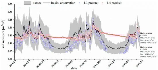
Figure 2. Time series of daily areal average values of the SMAP L3 and L4 products and in situ observation in the study area.

It is worth mentioning that, in winter (from December to March), the L3 product lacked data and the L4 product provided unreliable estimates with a linear trend showing significantly overestimations. The details of seasonal differences are shown in Table 4. Both the L3 and L4 products performed best in autumn, then followed by summer and spring. Evaluated by the combination of R, RMSE, absolute bias and ubRMSE values, the L3 product fits the observation better than the L4 product in spring, summer and autumn.

Table 4. Evaluation of daily average values from the SMAP L3 and L4 products at seasonal scale.

Seasons	The L3 Product					The L4 Product
	R	RMSE (m3/m3)	Bias (m3/m3)	ubRMSE (m3/m3)	n	R	RMSE (m3/m3)	Bias (m3/m3)	ubRMSE (m3/m3)	n
Spring	0.712	0.045	−0.039	0.022	216	0.052	0.033	0.001	0.033	245
Summer	0.735	0.028	−0.011	0.026	198	0.634	0.026	−0.010	0.024	205
Autumn	0.878	0.030	−0.022	0.020	168	0.522	0.039	0.022	0.032	182
Winter	--	--	--		0	−0.062	0.075	0.074	0.012	181

4.4. Temporal Stability Analysis

The temporal stability analysis is applied in this study because it is less influenced by sampling size and not so much dependent on the absolute values of soil moisture, but rather accounts for the tempo-spatial distributions of soil moisture [11]. The MRDs and their standard deviations of both the L3 and L4 products are shown in Figure 3. The L3 product has MRDs between −0.489 and 0.902, and for the L4 product the range of MRDs is from −0.438 to 0.945. The standard deviations of the L3 MRDs are quite high, ranging from 0.099 to 0.371 with mean value over all pixels of 0.184. For the L4 product, the standard deviations of MRDs range from 0.027 to 0.137 with an areal mean value of 0.072. Compared to the L4 product, the higher ranges of MRDs and higher standard deviations of the L3 product imply more dynamic in its tempo-spatial distributions.

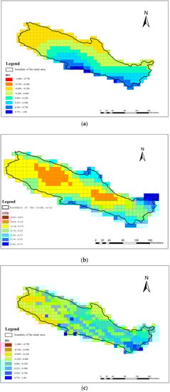
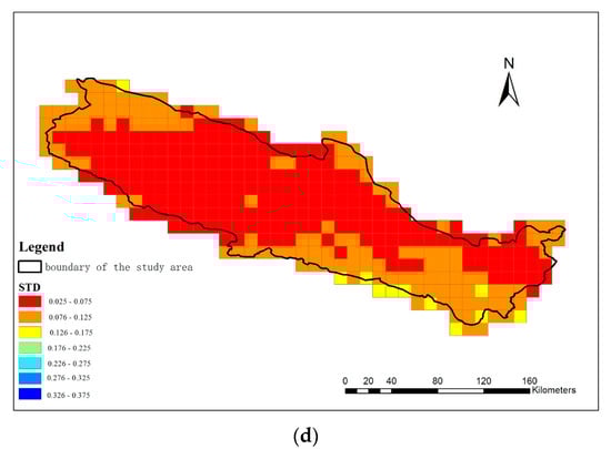
Figure 3. Temporal stability analysis of the SMAP L3 and L4 products. (a) mean relative differences (MRDs) of the L3 product; (b) standard deviation of the L3 product; (c) MRDs of the L4 product; (d) standard deviation of the L4 product.

For the L3 product, the MRDs are presented as smaller in the northwest and larger in the southeast, indicating that the estimates are drier in the northwest and wetter in the southeast. For the L4 product, the MRDs are smaller in the west and slightly larger in the east, which means that the estimates are drier in the west and wetter in the east. The precipitation in the study area shows increasing trends from northwest to southeast [42,43], leading to same spatial pattern of soil moisture. Thus, the L3 product better catches the spatial pattern of soil moisture in the study area. For both products, the standard deviations are smaller in central areas and larger in outlying areas. This implies lower persistence of soil moisture distributions over time in outlying areas than in central areas for both products. Nevertheless, the standard deviations of the L4 product show significantly smaller range, indicating that the L4 product had greater persistence of soil moisture distributions over time than the L3 product (Figure 3).

5. Discussion

5.1. Impacts of Uncertainties in Retrieval Algorithms

In the SMAP mission, the tau-omega model has been applied to describe the components from the soil, and the vegetation canopy contributes to the L-band brightness temperature [9,14]. If the air, vegetation, and near surface soil can be assumed to be in thermal equilibrium, then the vegetation temperature (T_C) is approximately equal to soil effective temperature (Ts), and both temperatures T_C and Ts can be replaced by the single effective temperature for the scene (T_eff) in the radiative transfer equation. To retrieve soil moisture data, it is necessary to isolate the soil surface emissivity $e_p$ in Formula (8) by inversion of the tau-omega model.

$$e_p=\frac{e-(1-{\omega }_p)(1-{\gamma }^2)}{(1-{\omega }_p){\gamma }^2+{\omega }_p\gamma }$$

(8)

where

$$e=\frac{T_{Bp}}{T_{eff}}$$

(9)

and

$$\gamma =\exp (-{\tau }_p\sec \theta )$$

(10)

and T_Bp is the brightness temperature of each SMAP grid cell, ${\tau }_p$ is the nadir vegetation opacity, ${\omega }_p$ is the vegetation effective scattering albedo, $\theta$ is the surface incidence angle of 40°. Based on the derived value of $e_p$, the smooth surface soil emissivity is determined by removing the roughness effects, and then soil moisture can be retrieved based on Fresnel equation and dielectric mixing model. Therefore, the accuracy of T_Bp and T_eff, as well as the suitability of ${\tau }_p$ and ${\omega }_p$ are crucial for the retrieval of soil moisture data [9,14].

There are uncertainties in estimating both T_Bp and T_eff in the SMAP mission. In mountainous areas, angles of incidence in the target area could not be derived solely from the radiometer observation angle, and the surrounding reflection significantly affects brightness temperature simulation [44]. Nevertheless, both of them have been ignored in the SMAP mission [14]. Meanwhile, the L3_SM_P_E product with a resolution of 9 km by 9 km, has been retrieved from the downscaled brightness temperatures in the L2_SM_P product [45]. The downscaling algorithms would cause uncertainties in T_Bp estimates, especially in areas with complex land surface conditions [45,46]. In the SMAP mission, the effective temperature T_eff has been provided by the GMAO (GSFC Global Modeling and Assimilation Office) model, also with unclear uncertainty. Moreover, the uncertainties of both T_Bp and T_eff would propagate through the soil moisture inversion algorithm [45], which is still unclear and requires further investigations in the future. Therefore, although well catching the temporal trend of in situ observations, both the L3 and L4 products did not achieve the accuracy of 0.04 m³/m³ at each overpassing moment in the study area.

The L3 product shows “dry bias” for all the vegetation types at each overpassing moment in this study, which has also been revealed at both footprint scale and global scale in previous studies, especially in mountainous areas (Table 5). Colliander et al. [12] attributed the “dry bias” to growth effects of vegetation. However, as shown in Table 6, both the L3 ascending and descending products underestimated soil moisture for all the vegetation types in both growing seasons (summer and autumn) and non-growing season (spring), with even larger underestimation in non-growing season. It implies that the “dry bias” is more related to the system structure of retrieval algorithms rather than the growth effects. Both ${\tau }_p$ and ${\omega }_p$ are the factors describing vegetation effects, and the retrieval parameters of them have been trained or validated by observations from the CVS [12], thus they can be assumed approximately precise at the CVS. However, the evaluations of the SMAP product at the CVS also show the “dry bias” [12]. Therefore, the “dry bias” of the SMAP L3 product is mainly caused by the uncertainties of the T_Bp and T_eff estimates rather than other factors. Furthermore, because the assumptions of thermal equilibrium are more likely to be true at the 6 a.m. SMAP overpass [9,14], the L3 ascending product fits the observation better than the L3 descending product.

Table 5. Evaluations of the SMAP products with in situ observations in previous studies.

Satellite Products	Study Area	Validation Period	R	RMSE (m3/m3)	Bias (m3/m3)	ubRMSE (m3/m3)	Reference
SMAP L2 product (9km)	Around the globe	13 April~6 July 2015	0.286~0.981	0.022~0.113	−0.070~0.075	0.018~0.084	[12]
SMAP L2 product (36 km)	the SMAP Validation Experiment 2015 in Southeast Arizona	1~18 August 2015	0.49	0.037	0.029	----	[21]
SMAP L2 product (36 km)	CVS	31 March~26 October 2015	0.719~0.781	0.061~0.071	−0.040~0.008	0.038~0.044	[13]
SMAP L3 product (9 km)	Genhe in China	15 July 2013~23 September 2016	0.498~0.713	0.039~0.063	−0.022~−0.050	----	[47]
SMAP L4 product (9 km)	the Great Plains region of the United States	1 April~1 December 2015	0.901	0.027	−0.001	----	[48]
SMAP L4 product (9 km)	Two in situ networks over the United States	April 2015~March 2016	0.54~0.8	0.09~0.15	----	0.09~0.12	[49]
SMAP L3 product (36 km)	Over China	1 April 2015~31 August 2016	0.44	0.108	0.058	0.059	[50]
SMAP L3_A product (3 km)	Cold and Arid Regions in Northwestern China	13 April~7 July 2015	0.214	0.17	−0.116	0.124	[51]
SMAP L3_AP product (9 km)			0.385	0.213	−0.203	0.067
SMAP L3_P product (36 km)		2 April~31 December 2015	0.498	0.098	−0.087	0.045
SMAP L3_P product (36 km)	Three networks over United States and Europe	1 April~1 December 2015	0.764	0.052	0.016	0.036	[52]

Table 6. Evaluation of the SMAP L3 products of both ascending and descending orbits at seasonal scale.

Vegetation Types	Seasons	Ascending				Descending
		R	RMSE (m3/m3)	bias (m3/m3)	n	R	RMSE (m3/m3)	bias (m3/m3)	n
Alpine meadow	Spring	0.568 *	0.133	−0.112	34	0.275	0.118	−0.094	55
	Summer	0.740 *	0.159	−0.154	81	0.766 *	0.160	−0.154	90
	Autumn	0.953 *	0.148	−0.145	46	0.834 *	0.152	−0.149	57
	Winter	--	--	--	0	--	--	--	0
Sparse grassland	Spring	0.466 *	0.045	−0.008	688	0.394 *	0.050	−0.013	816
	Summer	0.655 *	0.044	−0.002	1042	0.515 *	0.052	−0.017	1050
	Autumn	0.644 *	0.040	−0.013	672	0.520 *	0.045	−0.021	721
	Winter	--	--	--	0	--	--	--	0
Dense grassland	Spring	0.489 *	0.055	−0.041	701	0.460 *	0.052	−0.036	853
	Summer	0.659 *	0.052	−0.010	1096	0.611 *	0.058	−0.022	1142
	Autumn	0.689 *	0.051	−0.019	624	0.682 *	0.048	−0.016	728
	Winter	--	--	--	0	--	--	--	0
Shrub	Spring	0.016	0.268	−0.263	102	0.439 *	0.272	−0.268	112
	Summer	0.487 *	0.171	−0.159	176	0.514 *	0.176	−0.166	182
	Autumn	0.020	0.185	−0.167	94	0.096	0.179	−0.165	102
	Winter	--	--	--	0	--	--	--	0
Coniferous forest	Spring	0.579 *	0.053	−0.038	151	0.436 *	0.053	−0.032	192
	Summer	0.808 *	0.046	−0.037	218	0.728 *	0.056	−0.046	228
	Autumn	0.785 *	0.043	−0.036	181	0.741 *	0.040	−0.029	222
	Winter	--	--	--	0	--	--	--	0
Cropland	Spring	0.719 *	0.080	−0.078	69	0.710 *	0.076	−0.073	83
	Summer	0.817 *	0.055	−0.049	101	0.773 *	0.067	−0.061	100
	Autumn	0.722 *	0.066	−0.062	59	0.666 *	0.056	−0.052	63
	Winter	--	--	--	0	--	--	--	0
Barren land	Spring	0.496 *	0.077	−0.029	135	0.426 *	0.08	−0.040	167
	Summer	0.688 *	0.058	−0.012	275	0.661 *	0.065	−0.024	301
	Autumn	0.782 *	0.058	−0.005	153	0.662 *	0.059	−0.015	179
	Winter	--	--	--	0	--	--	--	0
In total	Spring	0.470 *	0.068	−0.043	1880	0.431 *	0.069	−0.044	2278
	Summer	0.670 *	0.059	−0.023	2989	0.593 *	0.066	−0.035	3093
	Autumn	0.659 *	0.058	−0.030	1829	0.596 *	0.058	−0.032	2072
	Winter	--	--	--	0	--	--	--	0

Note: No data of the SMAP product in winter. * refers to passing significance test of 0.001.

5.2. Impacts of Parameters b_p and h under Different Vegetation Types

According to Formula (8), ${\tau }_p$ and ${\omega }_p$ are two important factors related to vegetation effects [9,14]. In the SMAP mission, the nadir vegetation opacity ${\tau }_p$ is related to the total columnar vegetation water content W (kg/m²) by ${\tau }_p=b_{p}W$ with the coefficient b_p dependent on vegetation type [9,14]. Both b_p and ${\omega }_p$ have been determined before launch [12,14]. Meanwhile, surface soil reflectivity $r_p$, related to the soil emissivity $e_p$ by $e_p=1{-r}_p$, has been smoothed by $r_p^{smooth}{=r}_p^{rough}/\exp (-h)$ in the SMAP retrieval. As a linear function of the root mean square of surface heights, surface roughness h is also an important factor for soil moisture estimation in mountainous area [51,53].

As the parameters ${\omega }_p$ and b_p are functions of vegetation geometry and vegetation water content, both of them are important factors affecting the performance under vegetation conditions. Better characterizing parameter ${\omega }_p$ is important in soil moisture retrievals from space-borne observations [54,55,56,57]. However, as shown in Table 7, differing significantly in the values of ${\omega }_p$, both the SMAP L3 and L4 products show same performance trends under different vegetation types in the study area. Thus, the effects of ${\omega }_p$ on the performance differences of both products under different vegetation types are not discussed in this study.

Table 7. Values of ${\omega }_p$ used in both the SMAP L3 and L4 products under different vegetation types in the study area.

Vegetation Types	The L3 Product	The L4 Product
Alpine meadow	0.050	0.07
Sparse grassland	0.050	0.07
Dense grassland	0.050	0.07
Shrub	0.050	0.12
Coniferous forest	0.050	0.12
Cropland	0.050	0.12
Barren land	0.000	----

The b_p factor is more sensitive than surface roughness h in vegetated condition, thus the b_p factor is the most important parameter in soil moisture retrieval of the SMAP product for vegetation [58]. In the study area, the main crop is corn in cropland, which has been considered in the SMAP mission [14,59], thus leading to best performance in cropland in the study area far beyond the accuracy of 0.04 m³/m³. For coniferous forest, the parameters of evergreen needle leaf have been calibrated and validated by the CanExSM10 (The Canadian Experiment for Soil Moisture in 2010) measurements [14,60,61]. The main tree types are pine and spruce over the BERMS (Boreal Ecosystem Research and Monitoring Sites) forested sites in CanExSM10 [61], both of them are coniferae as well as picea crassifolia in our study area. Thus, the parameters of forest are suitable in the study area because of the similarity of tree species, resulting in better performance of the SMAP products in coniferous forest far beyond the accuracy of 0.04 m³/m³.

The parameters of grasslands have also been considered in the SMAP mission [14,62], but performed not as well as in coniferous forest. This is because the b_p factor varies depending on different soil and vegetation conditions [58], but only average values for each type have been applied in the SMAP mission [14,62]. Compared with the coniferous forest, the invariable b_p factor results in worse performance because of stronger intra-annual variation in grasslands (alpine meadow, sparse and dense grasslands). Since the brightness temperature shows higher sensitivity to vegetation under wet soil conditions [9,63], the misevaluation impacts of the b_p factor are much more significant in wet conditions [61,64]. Because of the wetness conditions of three grasslands (Table 8 and Figure 4), the L3 product shows best performance in sparse grassland under the driest condition, then dense grassland, and alpine meadow under the wettest condition.

Table 8. Statistics of in-situ observation under different vegetation types.

Statistics (m3/m3)	Alpine Meadow	Sparse Grassland	Dense Grassland	Shrub	Coniferous Forest	Cropland	Barren Land
Minimum	0.018	0.002	0.052	0.177	0.048	0.137	0.026
Maximum	0.477	0.370	0.424	0.627	0.294	0.295	0.339
Average	0.295	0.112	0.174	0.355	0.145	0.204	0.151
CV	0.254	0.587	0.311	0.243	0.319	0.143	0.474
Stdev	0.075	0.066	0.054	0.086	0.046	0.029	0.072

Note: CV refers to coefficient of variation.

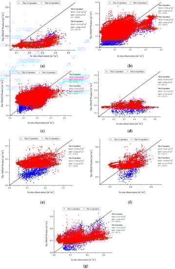
Figure 4. Scatterplots of the SMAP L3 and L4 products and in situ observation in the study area. (a) alpine meadow; (b) sparse grassland; (c) dense grassland; (d) shrub; (e) coniferous forest; (f) cropland; (g) barren land.

The SMAP L3 product shows poor performance in estimating soil moisture in shrub land. This is because the dominant species is potentilla fruticosa in the shrub land in the upper reach of the Heihe River Watershed, which belongs to the vegetation class of open shrublands in the SMAP mission. However, in the study area, the shrubland is often mixed with grassland, which leads to complexity in soil moisture retrieval. Moreover, potentilla fruticosa shows strong intra-annual variations because of growth effects. Thus, the invariable b_p factor results in errors of soil moisture retrievals in the shrubland. Meanwhile, the brightness temperature is much more sensitive to vegetation under wet soil conditions [9,63]. Under the wettest condition with higher soil moisture data in the shrub (Table 8 and Figure 4), the misevaluation impacts of the b_p factor is most significant and thus leading to worst performance in the shrub in the study area.

The L4 product is the assimilation results of the SMAP retrievals and the GEOS-5 model simulations, thus it shows similar performance with the L3 product under different vegetation types. Overall, the suitability as well as the variability of the b_p factor result in the performance differences of both the L3 and L4 products under different vegetation types in the study area. The impacts of the b_p factor is more significant under wet conditions, resulting in performance differences in the three grasslands with a declining order of sparse grassland, dense grassland and alpine meadow.

For barren land, compared to surface roughness and soil moisture, the backscatter weakly depends on soil type [65]. The uncertainties of surface roughness h dominate the error budget of T_Bp modeling over barren soil surface [53]. Meanwhile, although depending on surface soil moisture, the parameterization of h performs better when soil surface is relatively smooth than when the soil surface gets rougher [53]. Because of the complex topography in the study area, the errors in parameterization of h lead to poor performance of the SMAP products in barren land in the study area.

5.3. Impacts of Seasonal Frozen Soil

In the SMAP mission, the soil moisture data are retrieved by the relationship between soil moisture and dielectric constant. As soil moisture increases, the soil dielectric constant increases, which leads to an increase in soil reflectivity or a decrease in soil emissivity [14]. However, besides dry soil, low dielectric constant can also be associated with frozen soil which has a similar dielectric constant to dry soil independent of water content [14]. Thus, landscape freeze/thaw state is important in soil moisture data retrieval in the SMAP mission [66].

In the upper reach of the Heihe River Watershed, seasonal frozen soils account for about 65% of the study area [67], which strongly affects the soil moisture retrieval in the SMAP mission. In winter, the freeze_thaw_fraction values of all grids are near 1.0, leading to missing estimates, thus there is no data from the L3 product in the study area. For those frozen grids with estimates in the study area, the SMAP mission estimates unfrozen soil water, and the freeze_thaw_fraction values range from 0.008 to 0.892, the R values are 0.464 and 0.334 for the ascending and descending products, respectively, while the ubRMSE values are 0.051 and 0.053 m³/m³, respectively. Because the in situ soil moisture sensor 5TE can measure free water in frozen soil [68], the L3 product well catches the trend of observations under the frozen states. Under the unfrozen state, the R values are 0.624 and 0.555 for the ascending and descending products, respectively, and the corresponding ubRMSE values are 0.054 m³/m³ for both products. With slight differences in bias, the L3 product better catches the temporal trend of the in situ observations under the unfrozen state than the frozen state. Meanwhile, because of the soil frozen/thaw processes in spring in the study area, both the L3 and L4 products showed better performance in summer and autumn than in spring. However, the better performance of both products in autumn than in summer is caused by growth effects of the vegetation during the growing season.

5.4. Impacts of Assimilation System

The L4 product is soil moisture estimate by assimilating the SMAP observation (downscaled brightness temperature from L2 product) with simulation by a catchment land surface model, GEOS-5 [14]. The assimilation causes the performance differences in the L3 and L4 products. Because the L-band brightness temperatures generated by the GEOS-5 model and its associated microwave radiative transfer model have been calibrated to match the climatology of satellite observations, the GEOS-5 model provides unbiased modeled brightness temperatures in long-term mean ignoring seasonal variations in bias [17]. Meanwhile, the brightness temperature by the SMAP observations is converted to anomalies for assimilation by removing the climatology of satellite observations [17]. With lacking of SMAP-only climatology, the aforementioned climatology of satellite observations has been derived by the Soil Moisture and Ocean Salinity (SMOS) product, thus leading to the systemic errors of soil moisture estimates by the SMAP L4 product.

The calibration of the GEOS-5 model makes its simulation results more capable in reflecting the climatological trends with smaller variation. In winter, as there is no SMAP observed brightness temperature because of frozen states as for the L3 product, the estimates of the L4 product are all the simulation results by the GEOS-5 model, thus leading to linear temporal trends of the L4 product in winter. Also because of the better reflection in the climatological trends by the GEOS-5 model, the L4 product shows smaller variations with significantly smaller coefficient of variation (CV) values than the L3 product (Figure 4), thus the L3 product is more dynamic than the L4 product in catching the tempo-spatial distributions of soil moisture at the watershed scale.

In winter, the larger areal average values of soil moisture indicate that the GEOS-5 model overestimates soil moisture in the study area. This is because the GEOS-5 model has been calibrated over unfrozen land to simulate all the water in the soils [69]. However, the observed soil moisture is free water in the frozen soils, thus the values would be much smaller than the model simulations. Meanwhile, as shown in Table 4 and Figure 4, compared to the L3 product, the L4 product shows larger soil moisture estimates in all the seasons and under all the vegetation types. In the SMAP mission, the L3 product is the retrieval of downscaled (9-km) brightness temperatures, and the L4 product is assimilation result by retrieval of downscaled (9-km) brightness temperatures and GEOS-5 simulation. Because the same algorithm has been applied to retrieve soil moisture from brightness temperatures in both the L3 and L4 products, the larger estimates of the L4 product are mainly caused by the GEOS-5 model simulations. Moreover, the L3 product underestimates soil moisture in the study area, the overestimation of the L4 product indicates that the GEOS-5 model overestimates soil moisture in the study area. In summary, the assimilation makes the L4 product show similar temporal trends with the L3 product, but significantly differ in tempo-spatial distributions. Because of the relative errors of the SMAP brightness temperature observations and the corresponding land model forecast in the assimilation [14], the L3 product shows better performance than the L4 product in the study area under all the evaluation cases.

6. Conclusions

This paper presents evaluation of the SMAP L3 and L4 products under different vegetation types at multiple tempo-spatial scales over the upper reach of the Heihe River Watershed, Northwest China. The results are expected to increase the understanding of the suitability and the future improvements of the SMAP soil moisture products. Both products were compared with ground-based observations from a sparse in situ network from 1 April 2015 to 22 June 2017. Results show that both the L3 and L4 products well catch the temporal trend of the in situ observations in the study area. However, compared with in situ observations at point scale, both of them did not achieve the accuracy of 0.04 m³/m³ because of the uncertainties of brightness temperature T_Bp and effective temperature T_eff as well as their propagations in the inversion algorithm. Compared with areal average values at the watershed scale, the L3 product is far beyond the accuracy of 0.04 m³/m³ and the L4 product basically achieves the accuracy. The performance differences of both products at point scale and at watershed scale are caused by the scale mismatch in the evaluations, which is not discussed here because this study focuses on the impacts of vegetation types on the soil moisture estimates.

Almost all the evaluations show the “dry bias” of the SMAP product, it is more related to the aforementioned uncertainties of T_Bp and T_eff rather than the growth effects stated by Colliander et al. (2017a). Under different vegetation types, although both the L3 and L4 products catch the temporal trend of the observations well, the suitability and the variability of the b_p factor result in that both products performed best in cropland, then coniferous forest, sparse grassland, dense grassland, alpine meadow and worst in shrub. In barren land, the errors in estimating surface roughness h caused by the complex topography lead to poor performance of the SMAP product.

Although with similar temporal trends, the L3 and L4 products show different performance at both temporal and spatial scales, which are mainly caused by the assimilation system. Because the climatology of satellite observations used in the assimilation system has been derived by the SMOS product, the SMAP L4 product has systemic errors in soil moisture estimates. The calibration of the GEOS-5 model makes its simulation results more capable in reflecting the climatological trends with smaller variations, leading to larger variations of the L3 product than the L4 product in both temporal variations and spatial distributions. Moreover, the overestimations of soil moisture by the GEOS-5 model cause the overestimations of the L4 product. Although lacking data in winter, the L3 product well estimated the free soil water under both unfrozen state and frozen state. However, the L4 product provides unreliable estimates with a linear trend showing significantly overestimations in winter. Overall, because of the relative errors of the SMAP brightness temperature observations and the corresponding land model forecast in the assimilation, the L3 product provides more reliable soil moisture estimates with more dynamic spatial patterns than the L4 product in the study area.

Based on the results of this study, the following suggestions are proposed for the future improvements of the SMAP products. First, it is necessary to quantify the uncertainties of the estimates of brightness temperature T_Bp and effective temperature T_eff to retrieve more reliable soil moisture data. Second, the suitable values of coefficient b_p and surface roughness h are crucial in soil moisture retrievals, it is essential to determine b_p factor and h factor under various conditions in the future, especially for vegetation types with strong intra-annual variations. Finally, both the SMAP-only climatology and improvements of the GEOS-5 model are needed to improve the SMAP soil moisture estimates.

References

- Vereecken, H.; Huisman, J.A.; Pachepsky, Y.; Montzka, C.; van der Kruk, J.; Bogena, H.; Weihermüller, L.; Herbst, M.; Martinez, G.; Vanderborght, J. On the spatiotemporal dynamics of soil moisture at the field scale. J. Hydrol. 2014, 516, 76–96. [Google Scholar] [CrossRef]
- Petropoulos, G.P.; Ireland, G.; Barrett, B. Surface soil moisture retrievals from remote sensing: Current status, products & future trends. Phys. Chem. Earth 2015, 83–84, 36–56. [Google Scholar] [CrossRef]
- World Meteorological Organization; United Nations Eductional, Scientific and Cultural Organization; United Nations Environment Programme; International Council for Science. Implementation Plan for the Global Observing System for Climate in Support of the UNFCCC; Technical Report World Climate Observing System; World Meteorological Organization (WMO): Geneva, Switzerland, 2010.
- Srivastava, P.K.; Han, D.; RicoRamirez, M.A.; Islam, T. Appraisal of SMOS soil moisture at a catchment scale in a temperate maritime climate. J. Hydrol. 2013, 498, 292–304. [Google Scholar] [CrossRef]
- Al-Yaari, A.; Wigneron, J.-P.; Ducharne, A.; Kerr, Y.; de Rosnay, P.; de Jeu, R.; Govind, A.; Al Bitar, A.; Albergel, C.; Muñoz-Sabater, J.; et al. Global-scale evaluation of two satellite-based passive microwave soil moisture datasets (SMOS and AMSR-E) with respect to Land Data Assimilation System estimates. Remote Sens. Environ. 2014, 149, 181–195. [Google Scholar] [CrossRef]
- Wagner, W.; Lemoine, G.; Rott, H. A method for estimating soil moisture from ERS scatterometer and soil data. Remote Sens. Environ. 1999, 70, 191–207. [Google Scholar] [CrossRef]
- Kerr, Y.H.; Waldteufel, P.; Wigneron, J.P.; Martinuzzi, J.M.; Font, J.; Berger, M. Soil moisture retrieval from space: The Soil Moisture and Ocean Salinity (SMOS) mission. IEEE Trans. Geosci. Remote Sens. 2001, 39, 1729–1735. [Google Scholar] [CrossRef]
- Owe, M.R.; de Jeu, R.; Walker, J. A methodology for surface soil moisture and vegetation optical depth retrieval using the microwave polarisation difference index. Geosci. Remote Sens. 2001, 39, 1643–1654. [Google Scholar] [CrossRef]
- Entekhabi, D.; Njoku, E.G.; O’Neill, P.E.; Kellogg, K.H.; Crow, W.T.; Edelstein, W.N.; Entin, J.K.; Goodman, S.D.; Jackson, T.J.; Johnson, J.; et al. The Soil Moisture Active Passive (SMAP) Mission. Proc. IEEE 2010, 98, 704–716. [Google Scholar] [CrossRef]
- Jackson, T.J.; Cosh, M.H.; Bindlish, R.; Starks, P.J.; Bosch, D.D.; Seyfried, M.; Goodrich, D.C.; Moran, M.S.; Du, J. Validation of advanced microwave scanning radiometer soil moisture products. IEEE Trans. Geosci. Remote Sens. 2010, 48, 4256–4272. [Google Scholar] [CrossRef]
- Rötzer, K.; Montzka, C.; Bogena, H.; Wagner, W.; Kerr, Y.H.; Kidd, R.; Vereecken, H. Catchment scale validation of SMOS and ASCAT soil moisture products using hydrological modeling and temporal stability analysis. J. Hydrol. 2014, 519, 934–946. [Google Scholar] [CrossRef]
- Colliander, A.; Jackson, T.J.; Bindlish, R.; Chan, S.; Das, N.; Kim, S.B.; Cosh, M.H.; Dunbar, R.S.; Dang, L.; Pashaian, L.; et al. Validation of SMAP surface soil moisture products with core validation sites. Remote Sens. Environ. 2017, 191, 215–231. [Google Scholar] [CrossRef]
- Chan, S.K.; Bindlish, R.; O’Neill, P.E.; Njoku, E.; Jackson, T.; Colliander, A.; Chen, F.; Burgin, M.; Dunbar, S.; Piepmeier, J.; et al. Assessment of the SMAP Passive Soil Moisture Product. IEEE Trans. Geosci. Remote Sens. 2016, 54, 4994–5006. [Google Scholar] [CrossRef]
- Entekhabi, D.; Yueh, S.; O’Neill, P.E.; Kellogg, K.H.; Allen, A.; Bindlish, R.; Brown, M.; Chan, S.; Colliander, A.; Crow, W.T.; et al. SMAP Handbook; The National Aeronautics and Space Administration: Wsahington, DC, USA, 2014.
- Brown, M.E.; Escobar, V.; Moran, S.; Entekhabi, D.; O’Neill, P.E.; Njoku, E.G.; Doorn, B.; Entin, J.K. NASA’s Soil Moisture Active Passive (SMAP) Mission and Opportunities for Applications Users. Bull. Am. Meteorol. Soc. 2013, 94, 1125–1128. [Google Scholar] [CrossRef]
- Vreugdenhil, M.; Dorigo, W.; Broer, M.; Haas, P.; Eder, A.; Hogan, P.; Bloeschl, G.; Wagner, W. Towards a high-density soil moisture network for the validation of SMAP in Petzenkirchen, Austria. In Proceedings of the IGARSS 2013 IEEE International Geoscience and Remote Sensing Symposium, Melbourne, Australia, 21–26 July 2013. [Google Scholar]
- Reichle, R.; Koster, R.; De Lannoy, G.; Crow, W.; Kimball, J. Algorithm Theoretical Basis Document Level 4 Surface and Root Zone Soil Moisture (L4_SM) Data Product; The National Aeronautics and Space Administration (NASA): Wsahington, DC, USA, 2014.
- O’Neill, P.; Chan, S.; Colliander, A.; Dunbar, S.; Njoku, E.; Bindlish, R.; Chen, F.; Jackson, T.; Burgin, M.; Piepmeier, J.; et al. Evaluation of the validated Soil Moisture product from the SMAP radiometer. In Proceedings of the IGARSS 2016 IEEE International Geoscience and Remote Sensing Symposium, Beijing, China, 10–15 July 2016; pp. 125–128. [Google Scholar]
- Pan, M.; Cai, X.; Chaney, N.W.; Entekhabi, D.; Wood, E.F. An initial assessment of SMAP soil moisture retrievals using high-resolution model simulations and in situ observations. Geophys. Res. Lett. 2016, 43, 9662–9668. [Google Scholar] [CrossRef]
- Al-Yaari, A.; Wigneron, J.-P.; Kerr, Y.; Rodriguez-Fernandez, N.J.; O’Neill, P.E.; Jackson, T.J.; De Lannoy, G.J.M.; Al Bitar, A.; Mialon, A.; Richaume, P.; et al. Evaluating soil moisture retrievals from ESA’s SMOS and NASA’s SMAP brightness temperature datasets. Remote Sens. Environ. 2017, 193, 257–273. [Google Scholar] [CrossRef]
- Colliander, A.; Cosh, M.H.; Misraa, S.; Jackson, T.J.; Crow, W.T.; Chan, S.; Bindlish, R.; Chae, C.; Collins, C.H.; Yueh, S.H. Validation and scaling of soil moisture in a semi-arid environment: SMAP validation experiment 2015 (SMAPVEX15). Remote Sens. Environ. 2017, 196, 101–112. [Google Scholar] [CrossRef]
- Jin, M.; Zheng, X.; Jiang, T.; Li, X.; Li, X.; Zhao, K. Evaluation and Improvement of SMOS and SMAP Soil Moisture Products for Soils with High Organic Matter over a Forested Area in Northeast China. Remote Sens. 2017, 9, 387. [Google Scholar] [CrossRef]
- Chen, F.; Crow, W.T.; Colliander, A.; Cosh, M.; Jackson, T.J.; Bindlish, R.; Reichle, R. Application of triple collocation in ground-based validation of soil moisture active/passive (SMAP) Level 2 data products. IEEE J. Sel. Top. Appl. Earth Obs. Remote Sens. 2017, 10, 489–502. [Google Scholar] [CrossRef]
- Qi, S.; Luo, F. Land-use change and its environmental impact in the Heihe River Basin, arid northwestern China. Environ. Geol. 2006, 50, 535–540. [Google Scholar] [CrossRef]
- Zhang, L.; He, C.; Li, J.; Wang, Y.; Wang, Z. Comparison of IDW and physically-based IDEW method in hydrological modelling for a large mountainous watershed, Northwest China. River Res. Appl. 2017, 33, 912–924. [Google Scholar] [CrossRef]
- Geng, X.; Wang, X.; Yan, H.; Zhang, Q.; Jin, G. Land Use/Land Cover Change Induced Impacts on Water Supply Service in the Upper Reach of Heihe River Basin. Sustainability 2015, 7, 366–383. [Google Scholar] [CrossRef]
- Li, Z.; Xu, Z.; Shao, Q.; Yang, J. Parameter estimation and uncertainty analysis of SWAT model in upper reaches of the Heihe river basin. Hydrol. Process. 2009, 23, 2744–2753. [Google Scholar] [CrossRef]
- Gao, B.; Qin, Y.; Wang, Y.; Yang, D.; Zheng, Y. Modeling Ecohydrological Processes and Spatial Patterns in the Upper Heihe Basin in China. Forests 2016, 7, 10. [Google Scholar] [CrossRef]
- Kang, J.; Jin, R.; Li, X.; Ma, C.; Qin, J.; Zhang, Y. High spatio-temporal resolution mapping of soil moisture by integrating wireless sensor network observations and MODIS apparent thermal inertia in the Babao River Basin, China. Remote Sens. Environ. 2017, 191, 232–245. [Google Scholar] [CrossRef]
- González-Zamora, Á.; Sánchez, N.; Martínez-Fernández, J.; Gumuzzio, Á.; Piles, M.; Olmedo, E. Long-term SMOS soil moisture products: A comprehensive evaluation across scales and methods in the Duero Basin (Spain). Phys. Chem. Earth 2015, 83–84, 123–136. [Google Scholar] [CrossRef]
- Kerr, Y.H.; Al-Yaari, A.; Rodriguez-Fernandez, N.; Parrens, M.; Molero, B.; Leroux, D.; Bircher, S.; Mahmoodi, A.; Mialon, A.; Richaume, P.; et al. Overview of SMOS performance in terms of global soil moisture monitoring after six years in operation. Remote Sens. Environ. 2016, 180, 40–63. [Google Scholar] [CrossRef]
- Bai, X.; Zhang, L.; Wang, Y.; Tian, J.; He, C.; Liu, G. Variations of Soil Moisture Under Different Land Use and Land Cover Types in the Qilian Mountain, China. Res. Soil Water Conserv. 2017, 24, 17–25. (In Chinese) [Google Scholar] [CrossRef]
- Tian, J.; Zhang, B.; He, C.; Yang, L. Variability in Soil Hydraulic Conductivity and Soil Hydrological Response under Different Land Covers in the Mountainous Area of the Heihe River Watershed, Northwest China. Land Degrad. Dev. 2017, 28, 1437–1449. [Google Scholar] [CrossRef]
- Jin, X.; Zhang, L.; Gu, J.; Zhao, C.; Tian, J.; He, C. Modeling the Impacts of Spatial Heterogeneity in Soil Hydraulic Properties on Hydrologic Process in the Upper Reach of the Heihe River in the Qilian Mountains, Northwest China. Hydrol. Process. 2015, 29, 3318–3327. [Google Scholar] [CrossRef]
- Cobos, D.R.; Chambers, C. Calibrating ECH2O Soil Moisture Sensor; Application Note; Decagon Devices: Pullman, WA, USA, 2009. [Google Scholar]
- Albergel, C.; de Rosnay, P.; Gruhier, C.; Muñoz-Sabater, J.; Hasenauer, S.; Isaksen, L.; Kerr, Y.; Wagner, W. Evaluation of remotely sensed and modelled soil moisture products using global ground-based in situ observations. Remote Sens. Environ. 2012, 118, 215–226. [Google Scholar] [CrossRef]
- Wu, Q.; Liu, H.; Wang, L.; Deng, C. Evaluation of AMSR2 soil moisture products over the contiguous United States using in situ data from the International Soil Moisture Network. Int. J. Appl. Earth Obs. Geoinf. 2016, 45, 187–199. [Google Scholar] [CrossRef]
- Vachaud, G.; Silans, A.P.D.; Balabanis, P.; Vauclin, M. Temporal stability of spatially measured soil water probability density function. Soil Sci. Soc. Am. J. 1985, 49, 822–828. [Google Scholar] [CrossRef]
- Kachanoski, R.G.; Jong, E.D. Scale dependence and the temporal persistence of spatial patterns of soil water storage. Water Resour. Res. 1988, 24, 85–91. [Google Scholar] [CrossRef]
- Polcher, J.; Piles, M.; Gelati, E.; Barella-Ortiz, A.; Tello, M. Comparing surface-soil moisture from the SMOS mission and the ORCHIDEE land-surface model over the Iberian Peninsula. Remote Sens. Environ. 2016, 174, 69–81. [Google Scholar] [CrossRef]
- Galantowicz, J.F.; Entekhabi, D.; Njoku, E.G. Estimation of Soil-Type Heterogeneity Effects in the Retrieval of Soil Moisture from Radiobrightness. IEEE Trans. Geosci. Remote Sens. 2000, 38, 312–316. [Google Scholar] [CrossRef]
- Ding, Y.; Baisheng, Y.E.; Zhou, W. Temporal and Spatial Precipitation Distribution in the HeiheCatchment, Northwest China, During the Past 40 a. J. Glaciol. Geocryol. 1999, 21, 42–48. (In Chinese) [Google Scholar]
- Wang, C.; Zhao, C.Y. A Study of the Spatio-Temporal Distribution of Precipitation in Upper Reaches of Heihe River of China Using TRMM Data. J. Nat. Resour. 2013, 28, 862–872. (In Chinese) [Google Scholar]
- Pellarin, T.; Mialon, A.; Biron, R.; Coulaud, C.; Gibon, F.; Kerr, Y.; Lafaysse, M.; Mercier, B.; Morin, S.; Redor, I.; et al. Three years of L-band brightness temperature measurements in a mountainous area: Topography, vegetation and snowmelt issues. Remote Sens. Environ. 2016, 180, 85–98. [Google Scholar] [CrossRef]
- Das, N.N.; Entekhabi, D.; Dunbar, R.S.; Njoku, E.G.; Yueh, S.H. Uncertainty Estimates in the SMAP Combined Active-Passive Downscaled Brightness Temperature. IEEE Trans. Geosci. Remote Sens. 2016, 54, 640–650. [Google Scholar] [CrossRef]
- Wu, X.; Walker, J.P.; Das, N.N.; Panciera, R.; Rüdiger, C. Evaluation of the SMAP brightness temperature downscaling algorithm using active-passive microwave observations. Remote Sens. Environ. 2014, 155, 210–221. [Google Scholar] [CrossRef]
- Cui, H.; Jiang, L.; Du, J.; Zhao, S.; Wang, G.; Lu, Z.; Wang, J. Evaluation and analysis of AMSR-2, SMOS, and SMAP soil moisture products in the Genhe area of China. J. Geophys. Res. Atmos. 2017, 122, 8650–8666. [Google Scholar] [CrossRef]
- Bi, H.; Zeng, J.; Zheng, W.; Fan, X. Validation of SMAP Soil Moisture analysis product using in-situ measurements over the Little Washita Watershed. In Proceedings of the 2016 IEEE International Geoscience and Remote Sensing Symposium (IGARSS), Beijing, China, 10–15 July 2016. [Google Scholar]
- Zhang, X.; Zhang, T.; Zhou, P.; Shao, Y.; Gao, S. Validation Analysis of SMAP and AMSR2 Soil Moisture Products over the United States Using Ground-Based Measurements. Remote Sens. 2017, 9, 104. [Google Scholar] [CrossRef]
- Sun, Y.; Huang, S.; Ma, J.; Li, J.; Li, X.; Wang, H.; Chen, S.; Zang, W. Preliminary Evaluation of the SMAP Raiometer Soil Moisture Product over China Using In Situ Data. Remote Sens. 2017, 9, 292. [Google Scholar] [CrossRef]
- Ma, C.; Li, X.; Wang, J.; Wang, C.; Duan, Q.; Wang, W. A comprehensive Evaluation of Microwave Emissivity and Brightness Temperature Sensitivities to Soil Parameters Using Qualitative and Quantitative Sensitivity Analyses. IEEE Trans. Geosci. Remote Sens. 2017, 55, 1025–1038. [Google Scholar] [CrossRef]
- Zeng, J.; Chen, K.S.; Bi, H.; Chen, Q.; Yuan, L. A preliminary assessment of the SMAP radiometer soil moisture product using three in-situ networks. In Proceedings of the 2016 IEEE International Geoscience & Remote Sensing Symposium, Beijing, China, 10–15 July 2016. [Google Scholar]
- Peng, B.; Zhao, T.; Shi, J.; Lu, H.; Mialon, A.; Kerr, Y.H.; Liang, X.; Guan, K. Reappraisal of the roughness effect parameterization schemes for L-band radiometry over bare soil. Remote Sens. Environ. 2017, 199, 63–77. [Google Scholar] [CrossRef]
- Davenport, I.; Fernandez-Galvez, J.; Gurney, R. A sensitivity analysis of soil moisture retrieval from the tau–omega microwave emission model. IEEE Trans. Geosci. Remote Sens. 2005, 43, 1304–1316. [Google Scholar] [CrossRef]
- Van der Schalie, R.; Parinussa, R.; Renzullo, L.; van Dijk, A.; Su, C.-H.; de Jeu, R. SMOS soil moisture retrievals using the land parameter retrieval model: Evaluation over the Murrumbidgee Catchment, southeast Australia. Remote Sens. Environ. 2015, 163, 70–79. [Google Scholar] [CrossRef]
- Fernandez-Moran, R.; Wigneron, J.P.; Lopez-Baeza, E.; Al-Yaari, A.; Coll-Pajaron, A.; Mialon, A.; Mierneckid, M.; Parrens, M.; Salgado-Hernanz, P.M.; Schwank, M.; et al. Roughness and vegetation parameterizations at L-band for soil moisture retrievals over a vineyard field. Remote Sens. Environ. 2015, 170, 269–279. [Google Scholar] [CrossRef]
- Konings, A.G.; Piles, M.; Das, N.; Entekhabi, D. L-band vegetation optical depth and effective scattering albedo estimation from SMAP. Remote Sens. Environ. 2017, 198, 460–470. [Google Scholar] [CrossRef]
- Seo, D.; Lakhankar, T.; Khanbilvardi, R. Sensitivity Analysis of b-factor in Microwave Emission Model for Soil Moisture Retrieval A Case Study for SMAP Mission. Remote Sens. 2010, 2, 1273–1286. [Google Scholar] [CrossRef]
- Wigneron, J.P.; Parde, M.; Waldteufe, P.; Chanzy, A. Characterizing the dependence of vegetation model parameters on crop structure, incidence angle, and polarization at L-band. IEEE Trans. Geosci. Remote Sens. 2004, 42, 416–425. [Google Scholar]
- Tabatabaeenejad, A.; Burgin, M.; Moghaddam, M. Potential of L-band radar for retrieval of canopy and subcanopy parameters of boreal forests. IEEE Trans. Geosci. Remote Sens. 2012, 50, 2150–2160. [Google Scholar] [CrossRef]
- Djamai, N.; Magagi, R.; Goïta, K.; Hosseini, M.; Cosh, M.H.; Berg, A.; Toth, B. Evaluation of SMOS soil moisture products over the CanEx-SM10 area. J. Hydrol. 2015, 520, 254–267. [Google Scholar] [CrossRef]
- Njoku, E.G.; Wilson, W.J.; Yueh, S.H.; Dinardo, S.; Li, F.K.; Jackson, T.J.; Lakshmi, V.; Bolten, J. Observations of soil moisture using a passive and active low-frequency microwave airborne sensor during SGP99. IEEE Trans. Geosci. Remote Sens. 2002, 40, 2659–2673. [Google Scholar] [CrossRef]
- Ulaby, F.T.; Moore, R.K.; Fung, A.K. Microwave Remote Sensing: Active and Passive; Volume III, From Theory to Application; Artech House: Dedham, MA, USA, 1986. [Google Scholar]
- Gherboudj, I.; Magagi, R.; Goïta, K.; Berg, A.; Toth, B.; Walker, A. Validation of SMOS data over agricultural and boreal forest areas in Canada. IEEE Trans. Geosci. Remote Sens. 2012, 50, 1623–1635. [Google Scholar] [CrossRef]
- Oh, Y.; Sarabandi, K.; Ulaby, F.T. Semi-empirical model of the ensemble-averaged differential Mueller matrix for microwave backscattering from bare soil surfaces. IEEE Trans. Geosci. Remote Sens. 2002, 40, 1348–1355. [Google Scholar] [CrossRef]
- Derksen, C.; Xu, X.; Dunbar, R.S.; Colliander, A.; Kim, Y.; Kimball, J.S.; Black, T.A.; Euskirchen, E.; Langlois, A.; Loranty, M.M.; et al. Retrieving landscape freeze/thaw state from Soil Moisture Active Passive (SMAP) radar and radiometer measurements. Remote Sens. Environ. 2017, 194, 48–62. [Google Scholar] [CrossRef]
- Ning, B.Y.; He, Y.Q.; He, X.Z.; Li, Z.X. Advances on water resource research in Heihe river Basin. J. Desert Res. 2008, 28, 1180–1185. (In Chinese) [Google Scholar]
- Dente, L.; Vekerdy, Z.; Wen, J.; Su, Z. Maqu network for validation of satellite-derived soil moisture products. Int. J. Appl. Earth Obs. Geoinf. 2012, 17, 55–65. [Google Scholar] [CrossRef]
- De Lannoy, G.J.M.; Reichle, R.H.; Pauwels, V.R.N. Global Calibration of the GEOS-5 L-Band Microwave Radiative Transfer Model over Nonfrozen Land Using SMOS Observations. J. Hydrometeorol. 2013, 14, 765–785. [Google Scholar] [CrossRef]
© 2017 by the authors. Licensee MDPI, Basel, Switzerland. This article is an open access article distributed under the terms and conditions of the Creative Commons Attribution (CC BY) license (http://creativecommons.org/licenses/by/4.0/).