Gross Primary Production of a Wheat Canopy Relates Stronger to Far Red Than to Red Solar-Induced Chlorophyll Fluorescence

Abstract

Sun-induced chlorophyll fluorescence (SIF) is a radiation flux emitted by chlorophyll molecules in the red (RSIF) and far red region (FRSIF), and is considered as a potential indicator of the functional state of photosynthesis in remote sensing applications. Recently, ground studies and space observations have demonstrated a strong empirical linear relationship between FRSIF and carbon uptake through photosynthesis (GPP, gross primary production). In this study, we investigated the potential of RSIF and FRSIF to represent the functional status of photosynthesis at canopy level on a wheat crop. RSIF and FRSIF were continuously measured in the O₂-B (SIF687) and O₂-A bands (SIF760) at a high frequency rate from a nadir view at a height of 21 m, simultaneously with carbon uptake using eddy covariance (EC) techniques. The relative fluorescence yield (Fyield) and the photochemical yield were acquired at leaf level using active fluorescence measurements. SIF was normalized with photosynthetically active radiation (PAR) to derive apparent spectral fluorescence yields (ASFY687, ASFY760). At the diurnal scale, we found limited variations of ASFY687 and ASFY760 during sunny days. We also did not find any link between Fyield and light use efficiency (LUE) derived from EC, which would prevent SIF from indicating LUE changes. The coefficient of determination ($r^2$) of the linear regression between SIF and GPP is found to be highly variable, depending on the emission wavelength, the time scale of observation, sky conditions, and the phenological stage. Despite its photosystem II (PSII) origin, SIF687 correlates less than SIF760 with GPP in any cases. The strongest SIF–GPP relationship was found for SIF760 during canopy growth. When canopy is in a steady state, SIF687 and SIF760 are almost as effective as PAR in predicting GPP. Our results imply some constraints in the use of simple linear relationships to infer GPP from SIF, as they are expected to be better predictive with far red SIF for canopies with a high dynamic range of green biomass and a low LUE variation range.

1. Introduction

Terrestrial vegetation plays a major role at the Earth’s surface by harvesting sunlight and converting photons’ energy into a redox potential available to the rest of the biosphere. This basic process of energy conversion occurs in the antennae pigments of photosystems from the excited state of chlorophyll a (Chl a). In optimal conditions, the process is highly efficient, although a small part of the absorbed energy is re-emitted as fluorescence. This emission occurs in two broad bands in the red and far red parts of the spectrum, with maxima near 685 and 740 nm, respectively [1]. As fluorescence emission competes with photochemical conversion and heat dissipation of the excess energy, chlorophyll fluorescence (ChlF) has long been considered as a convenient non-intrusive probe to assess photosynthetic processes in chloroplasts and leaves (for a comprehensive review, see [2,3,4]). However, assessment of ChlF at larger scales has long been limited by the power of light sources that can be used to excite fluorescence from remote distances [5]. In the last decade, new methods for the remote sensing of ChlF at canopy level were developed to disentangle sun-induced fluorescence (SIF) from reflected light. Shortly, these methods take advantage of narrow absorption features of the solar spectrum—the so-called Fraunhofer lines—in which incident radiation is significantly reduced [6,7]; for a review, see [8]. As vegetation fluorescence is added to reflected light, it induces a small but detectable alteration of the absorption features, allowing the quantification of fluorescence. This “in-filling” approach has been successfully applied in the atmospheric absorption bands (namely, O₂-A and O₂-B) or in the solar Fraunhofer lines to detect vegetation fluorescence from various platforms at ground level [6,9,10,11,12], from an airborne platform [13,14], from an unmanned aerial vehicle (UAV) [15], and from space [16,17]. Recently, the European Space Agency (ESA) selected the FLEX (FLuorescence EXplorer) mission to be the 8th Earth Explorer in the framework of the Living Planet Program [18].

Using data from the GOSAT-TANSO (Greenhouse gases Observing SATellite-Thermal And Near-infrared Sensor for carbon Observation) instrument, a linear relationship between far red SIF (FRSIF) and gross primary production (GPP) was found on a monthly or yearly basis [16,19]. On a monthly basis, FRSIF from croplands in the US corn-belt strongly correlated with GPP estimated from flux towers, but deviated from model-based GPP. Hence, agricultural productivity is suspected to be severely underestimated by global GPP models [20]. According to these observations, SIF appears as a powerful indicator that can help to improve the assessment of plant productivity on a global basis. However, a better understanding of the complex interactions between the factors that contribute to canopy fluorescence is required to go beyond a simple empirical observation of an association between GPP and fluorescence radiance. So far, ChlF has been extensively studied at the chloroplast or leaf level, but observation of ChlF at the canopy level and its relationship with photosynthesis in natural conditions is still in its infancy [21]. In this context, outdoor ground studies based on continuous ChlF measurements over well-characterized ecosystems are essential experimental tools to capture the complex dynamic of SIF at both diurnal and seasonal scales. Using a high spectral resolution spectrometer, Rossini et al. [22] found a strong linear relationship ($r^2=0.80$) between SIF at 760 nm measured in the O₂-A band (SIF760) and GPP measured with eddy covariance (EC) techniques on a rice crop in an analysis over two complete vegetative cycles. This value of the correlation coefficient is close to the value found from space data in [16]. However, in their study, fluorescence measurements were acquired only at solar noon, and no information is provided about the diurnal dynamic of fluorescence and its interaction with GPP. In another study performed at ground level on a maize crop over four seasonal cycles, a much lower correlation between SIF760 and GPP was found ($r^2=0.30$) [23], which indicates that the correlation between SIF and GPP is subjected to changes, while the factors that control these variations remain unknown. Damm et al. [24] analyzed the full diurnal cycle of SIF and GPP, but their investigation was limited to a short period in the season, with no major phenological vegetation changes. In another study, the relationship between airborne SIF and GPP was found to be asymptotic and ecosystem-specific [25]. Spaceborne SIF is also used to constrain process-based vegetation models like SCOPE [26], with better simulations of GPP than other approaches based on vegetation indices [27,28]. However, the factors that drive the SIF–GPP relationship in different experimental conditions according, for example, to irradiance or phenology remains unclear, as studies on this topic are still rare. More specifically, the question remains as to what extent this relationship is due to absorbed photosynthetically active radiation (APAR) and/or light use efficiency (LUE) [29].

Moreover, most studies are limited to far red SIF (e.g., SIF760, measured in the O₂-A band at 760 nm), and very little information is available on the diurnal and seasonal dynamics of red SIF (RSIF, e.g., SIF687, measured in the O₂-B band at 687 nm) [23]. Compared to far red fluorescence, red fluorescence—produced dominantly by photosystem II (PSII)—is the most variable part of ChlF [30]. Hence, RSIF would be a preferential choice to assess physiologically-induced ChlF variations, and the detection of both peaks would provide complementary information on photosystem I (PSI) and PSII emissions [31]. In this study, we used the field platform for continuous measurements of fluorescence [32] located in Avignon, France to investigate both diurnal and seasonal dynamics of RSIF and FRSIF over a wheat crop during a complete vegetative cycle. SIF was continuously measured and retrieved from the O₂-B (SIF687) and O₂-A (SIF760) bands. Carbon fluxes were simultaneously monitored using eddy covariance techniques [33]. In most previous ground studies, SIF measurements were taken at a very low altitude (around 1 m above the canopy, see [22,23,24]). These experimental conditions are not truly representative of a remote sensing viewing configuration, because it implies either a limited sampled area (which is not representative of the whole canopy), or a large field of view, which encompasses different viewing angles. Here, we performed nadir measurements from the top of a crane at an altitude of 21 m with a relatively narrow low field of view (5°) to limit the extent of the viewing angles. Fluorescence was also assessed at leaf level using active measurements to derive information on fluorescence and photochemical yields.

The aims of the study are:

-

to investigate both diurnal and seasonal dynamics of RSIF and FRSIF during a complete vegetative cycle of a crop,

-

to analyze the relationship between SIF and GPP according to emission wavelength, time scale, and phenological stage,

-

to investigate the factors that potentially control the relationship between SIF and GPP using independent measurements of APAR on one hand, and of fluorescence and photochemical yield by active methods on the other hand.

2. Materials and Methods

2.1. Experimental Site

The study was conducted with the experimental field platform designed for the continuous measurement of vegetation fluorescence at the “Institut National de la Recherche Agronomique” (INRA) site located in Montfavet near Avignon, France (${43}^{\circ }$${55}^{\prime }$${3.24}^{″}$N, $4^{\circ }$${52}^{\prime }$${46.60}^{″}$E). The site is equipped with a movable crane, which can translate between two contiguous field plots of 100 × 200 ${\mathrm{m}}^2$ and 60 × 150 ${\mathrm{m}}^2$. Additional information on the site and instrumental equipment can be found in [32]. The two plots were sowed with winter wheat (Triticum turgidum durum, cultivar Daker) on 19 November 2009, with a plant density of 338 plants/${\mathrm{m}}^2$ and a distance between rows of $14.5\mathrm{c}\mathrm{m}$. Measurements were carried out from 3 March 2010 (day of year (DOY) 62) to 16 June 2010 (DOY 167). This time period goes roughly from the end of the tillering phase to the end of grain filling (Figure 1).

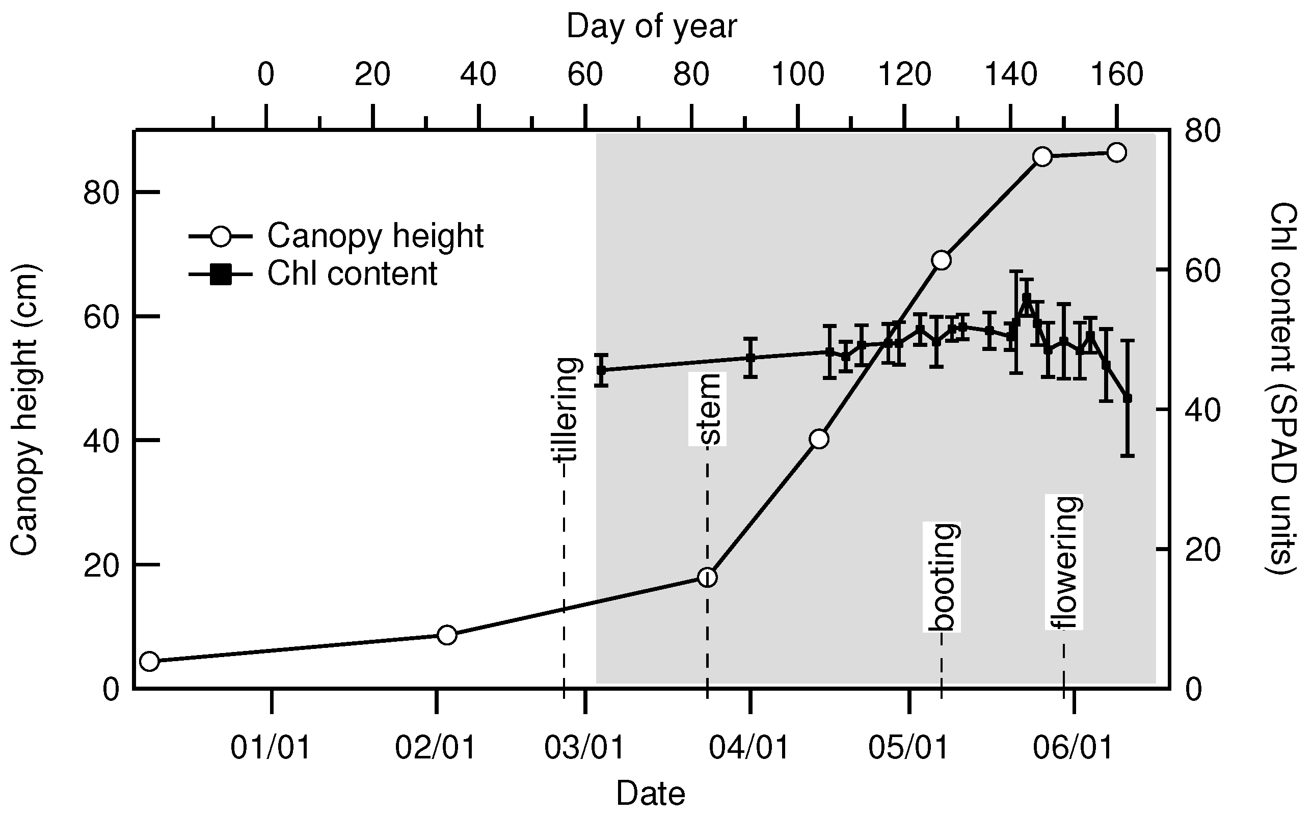
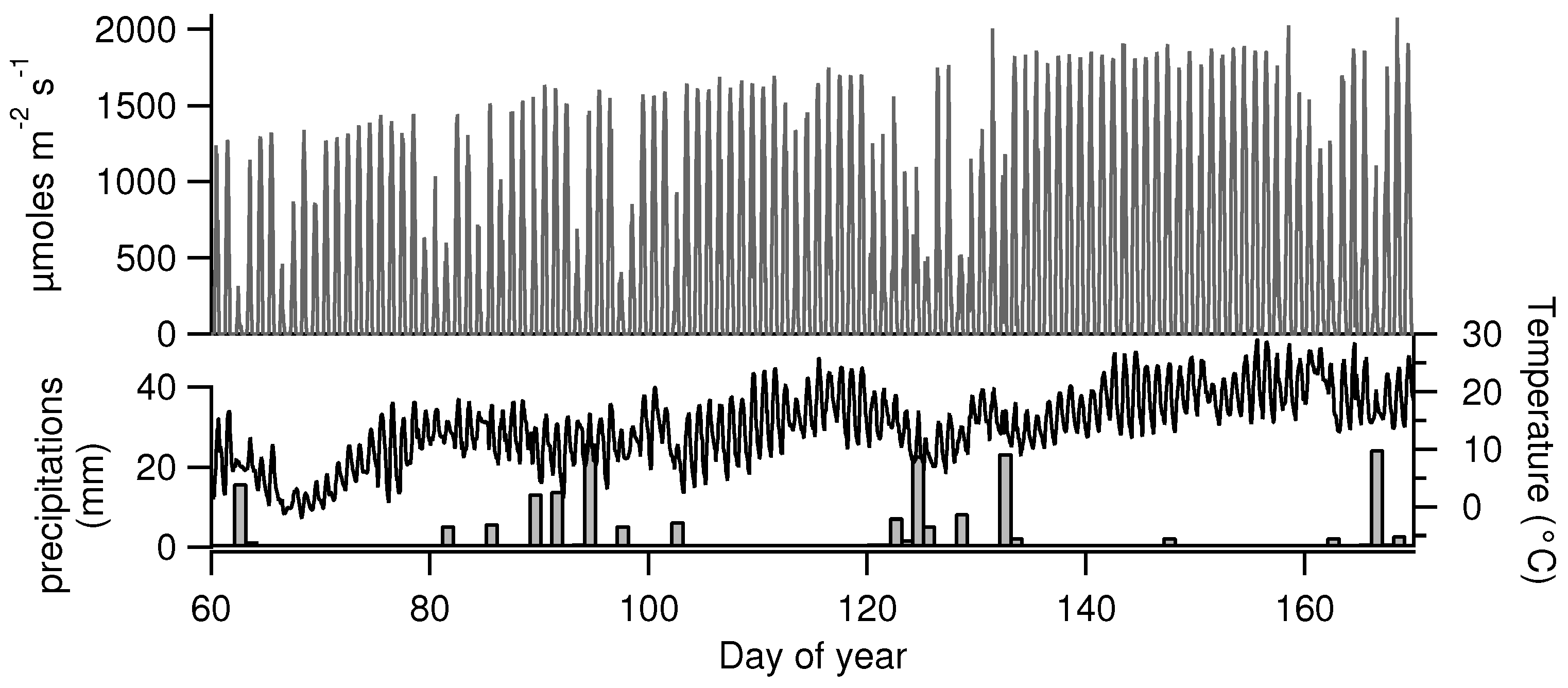
2.2. Canopy Characterization and Environmental Data

Leaf chlorophyll content was estimated with a chlorophyll meter SPAD-502 (Minolta, Ramsey, NJ, USA), and is expressed here in SPAD units, which presents a curvilinear relationship with chlorophyll content and roughly corresponds to it in $\mathsf{\mu }$g$·$${\mathrm{cm}}^{-2}$ [34]. Leaf fluorescence spectra under natural light were acquired with a specific laboratory-made device (leaf spectro-fluorometer, LSF) described elsewhere [13,35]. Briefly, it consists of a focusing optic that projects blue-green filtered sunlight on the leaf, so that the illumination intensity is equivalent to the outdoor incident photosynthetically active radiation (PAR). The fluorescence emission spectrum is detected from $660\mathrm{n}\mathrm{m}$ to $800\mathrm{n}\mathrm{m}$ with a compact spectrometer coupled with a fibre optic. Mean canopy height, fresh and dry above-ground biomass, and leaf area index (LAI) were measured at periodic intervals during crop development (

Table 1. Height, leaf area index (LAI), and aerial biomass of the crop at different dates during the measurement campaign.

Date	2 March	24 March	14 April	7 May	26 May	9 June
Day of Year	34	83	104	127	146	160
Height ($\mathrm{c}$$\mathrm{m}$)	8.6	18	40	69	86	86
LAI (${\mathrm{m}}^2$$·$${\mathrm{m}}^{-2}$)	0.15	0.89	3.32	6.88	5.74	1.07
Fresh biomass (kg$·$${\mathrm{m}}^{-2}$)	0.091	0.58	2.13	4.26	4.32	3.50
Dry biomass (kg$·$${\mathrm{m}}^{-2}$)	0.018	0.116	0.384	1.02	1.51	1.67

). LAI was assessed using a LI-3100 (Li-Cor, Lincoln, NE, USA) area meter. Incident PAR was measured at the same sampling rate as the vegetation radiance acquired by TriFLEX (see Section 2.3.1) with a quantum sensor (JYP 1000, SDEC, Reignac sur Indre, France). Half-hourly diffuse fraction of incident PAR was measured using a BF3 light sensor (Delta-T Devices, Cambridge, UK) and air temperature with a HPM35D sensor (Vaisala, Helsinki, Finland) (see Figure 2).

2.3. Passive Remote Sensing of SIF and Reflectance

2.3.1. Instrumental Setup and Retrieval of Fluorescence

Vegetation radiance was recorded with the TriFLEX instrument described in [32].The instrument was fixed at the top of the crane to observe vegetation from nadir. At the working height ($21\mathrm{m}$), the diameter of the observed area on top of the canopy was about $2\mathrm{m}$. Given the crop homogeneity, this measuring configuration can be considered as representative of true remote sensing conditions. Briefly, TriFLEX is a fluorosensor that uses two identical spectro-radiometers (HR2000+, $10\mathsf{\mu }\mathrm{m}$ entrance slit, full width at half-maximum (FWHM) $0.4\mathrm{n}\mathrm{m}$ at $687\mathrm{n}\mathrm{m}$ and $0.5\mathrm{n}\mathrm{m}$ at $760\mathrm{n}\mathrm{m}$, Ocean Optics, Dudenin, FL, USA) to simultaneously record the vegetation radiance and irradiance spectra in the chlorophyll emission band from $630\mathrm{n}\mathrm{m}$ to $815\mathrm{n}\mathrm{m}$ with a $0.09\mathrm{n}\mathrm{m}/\mathrm{pixel}$ sampling interval. With this setting, the time delay between vegetation and irradiance spectrum is reduced, enabling kinetic measurements of SIF. A third spectro-radiometer (HR2000+, $50\mathsf{\mu }\mathrm{m}$ entrance slit, FWHM $2\mathrm{n}\mathrm{m}$) alternatively measured vegetation radiance and solar irradiance on a broader spectral range from $300\mathrm{n}\mathrm{m}$ to $900\mathrm{n}\mathrm{m}$. Irradiance spectra were assessed by measuring radiance over a white reference surface made with a frosted polyvinyl chloride panel. The reflectance spectrum of the reference panel was determined in the laboratory against a reflectance standard (Spectralon, Labsphere, North Dutton, NH, USA), and further checked at the end of the measurements campaign to account for possible shifts induced by prolonged outdoors conditions. Each spectro-radiometer was connected to a fibre optic, which looks down to the vegetation at nadir with a field of view corresponding to a measured area of $2\mathrm{m}$ diameter. Vegetation and reference spectra were atmospherically corrected for the difference in altitude between ground and the reference panel using MODTRAN 4 [36]. The signal acquired on the vegetation was corrected to compensate for the absorption of the atmosphere along the path from vegetation to sensor, and the signal acquired on the reference board was corrected for the lack of absorption of incident light from the reference altitude to the ground. The two measured signals were corrected from these effects using MODTRAN 4, which computes the two transmission factors [37]. The variation of fluorescence flux induced by this atmospheric correction was about 5% for the O₂-A absorption band and 1.3% for the O₂-B band. Raw data were aggregated to a limited number of spectral channels designed to capture the essential features of each absorption band (three channels at 757.86, 760.51, and 770.46 $\mathrm{n}$$\mathrm{m}$ for the A band, four channels at 683.14, 685.00, 686.97, and 697.06 $\mathrm{n}$$\mathrm{m}$ for the B band), and were automatically saved on a remote server. Bandwidths of integration were from $0.1\mathrm{n}\mathrm{m}$ to $0.89\mathrm{n}\mathrm{m}$, according to channel (see [32] for details). SIF retrieval was performed with the algorithm proposed in [32] and described in Appendix A . In this method (called nFLD hereafter, where n is the number of measuring channels), fluorescence radiance at a given absorption band (SIF687 in the O₂-B band, SIF760 in the O₂-A band) is retrieved using a limited number (n) of measuring channels in each O₂ band and specific models of fluorescence and reflectance that apply only in the vicinity of each oxygen absorption band. We used three channels in the O₂-A band, and a polynomial of degree one to model the reflectance (i.e., a linear model), and four channels in the O₂-B band with a polynomial of degree two to model reflectance. In Appendix A, the retrieval errors were assessed on a simulated database of canopy and reference panel radiances with a known level of fluorescence. The mean retrieval error (${\overline{SIF}}_{bias}$), as well as the root mean square error (${\overline{SIF}}_{RMSE}$) computed from retrievals on a set of simulated top of canopy (TOC) radiances were found to be higher for SIF687 than for SIF760 (−0.038 vs. 0.015 mW$·$${\mathrm{m}}^{-2}·$${\mathrm{sr}}^{-1}·$${\mathrm{nm}}^{-1}$ for ${\overline{SIF}}_{bias}$, and $0.061$ vs. 0.022 mW$·$${\mathrm{m}}^{-2}·$${\mathrm{sr}}^{-1}·$${\mathrm{nm}}^{-1}$ for ${\overline{SIF}}_{RMSE}$, respectively, under a PAR irradiance of 1400 $\mathsf{\mu }$mol$·$${\mathrm{m}}^{-2}$$·$${\mathrm{s}}^{-1}$ (see Appendix A). These error values should be taken into account in the interpretation of the experimental results after PAR correction.

2.3.2. Derivation of Other Remote Sensing Parameters

Raw fluorescence and other optical data were averaged over $1\min$ time intervals in order to reduce the relative random error. This sampling rate allows for the discrimination of rapid changes in illumination caused by clouds. Wheat has a rather erectophile canopy architecture [38,39], and erectophile canopies are the most affected by bidirectional effects induced by changes in illumination. An additional averaging over $30\min$ was applied in order to synchronize fluorescence data with gas exchange measurements. We defined an apparent spectral fluorescence yield (ASFY) of the canopy (ASFY687, ASFY760) by dividing SIF expressed in quanta units ($\mathsf{\mu }$mol$·$${\mathrm{m}}^{-2}·$${\mathrm{sr}}^{-1}·$${\mathrm{nm}}^{-1}$) by PAR ($\mathsf{\mu }$mol$·$${\mathrm{m}}^{-2}$$·$${\mathrm{s}}^{-1}$) [9,40]. The factor π is used here to convert radiance units into irradiance units. Hence, ASFY is equivalent to a spectral density with units in $\mathrm{n}{\mathrm{m}}^{-1}$.

$$\mathrm{ASFYx}\left[\mathrm{n}{\mathrm{m}}^{-1}\right]=\frac{\pi \times \mathrm{SIFx}[\mathsf{\mu }\mathrm{mol}·{\mathrm{m}}^{-2}·{\mathrm{sr}}^{-1}·{\mathrm{nm}}^{-1}]}{\mathrm{PAR}[\mathsf{\mu }\mathrm{mol}·{\mathrm{m}}^{-2}·{\mathrm{s}}^{-1}]};x\in \{687,760\}$$

(1)

In a similar way, we defined the true spectral fluorescence yield (SFY) as:

$$\mathrm{SFYx}\left[\mathrm{n}{\mathrm{m}}^{-1}\right]=\frac{\pi \times \mathrm{SIFx}[\mathsf{\mu }\mathrm{mol}·{\mathrm{m}}^{-2}·{\mathrm{sr}}^{-1}·{\mathrm{nm}}^{-1}]}{\mathrm{APAR}[\mathsf{\mu }\mathrm{mol}·{\mathrm{m}}^{-2}·{\mathrm{s}}^{-1}]};x\in \{687,760\}$$

(2)

We also computed the Normalized Difference Vegetation Index (NDVI) from spectroscopic data as:

$$\mathrm{NDVI}=\frac{\rho 755-\rho 685}{\rho 755+\rho 685}$$

(3)

where ρ685 and ρ755 are the vegetation reflectance at $685\mathrm{n}\mathrm{m}$ and $755\mathrm{n}\mathrm{m}$, respectively.

2.4. Measurements of Canopy Transmittance and Absorbed PAR

Canopy transmittance was measured with a laboratory-made system which consists of ten quantum sensors (spectral bandwidth 400–700 nm) randomly distributed under the canopy at ground level. The transmitted irradiance $I_T$ was computed as the mean irradiance on the ten sensors averaged over time intervals of 30 min. An eleventh sensor measured the incident PAR at the top of the canopy in the same spectral band. APAR and the fraction of absorbed PAR (fAPAR) were computed from transmitted irradiance as:

$$\mathrm{fAPAR}=0.96\times (1-\frac{I_T}{\mathrm{PAR}})$$

(4)

$$\mathrm{APAR}=\mathrm{fAPAR}\times \mathrm{PAR}$$

(5)

The factor 0.96 results from the regression model between the true fAPAR (which requires the measurement of both transmitted and reflected light), and the fAPAR obtained here, which is deduced from transmitted light only [41].

2.5. Measurements of CO₂ Fluxes

The Avignon site is part of the CarboEurope-IP Regional Experiment [42] and the CarboEurope-IP Ecosystem Component. CO₂ fluxes were measured continuously using the eddy covariance (EC) technique at 30 min intervals by means of a Young 81000 3D sonic anemometer (Young, Traverse City, MI, USA) and a LI-7500 open path CO₂/H₂O analyzer (Li-Cor, Lincoln, NE, USA). We used Level 4 (i.e., quality-checked and gap-filled) data products from the CarboEurope database [33]. The footprint analysis suggests that—on average—85–90% of the fluxes originated from the studied field. Because EC measures Net Ecosystem Exchange (NEE), which is the algebraic sum of the CO₂ fixed by plants (GPP) and ecosystem respiration ($Re$), NEE was partitioned to derive GPP. For this purpose, day-time measurements were fitted to a hyperbolic dependence with PAR according to [43]:

$$\mathrm{NEE}=\frac{a_1\times \mathrm{PAR}}{a_2+\mathrm{PAR}}+R_e$$

(6)

with fitting parameters $a_1$, $a_2$, and $R_e$. With this formulation, the estimate of NEE at zero PAR gives the mean daytime respiration $R_e$, which was subsequently fit to an exponential function of temperature and extrapolated to daytime temperature. The mean value for $R_e$ during the measurement period was $4.6\pm 1.0\mathsf{\mu }\mathrm{mol}\mathrm{C}·{\mathrm{m}}^{-2}·{\mathrm{s}}^{-1}$ (1 sd). This is a rather moderate value compared to the total carbon flux. By subtracting $R_e$ from NEE, we computed the half-hourly average of GPP as:

$$\mathrm{GPP}=-\mathrm{NEE}+R_e$$

(7)

2.6. Active Fluorometry in the Field

Fluorescence parameters and incident PAR at the leaf level were obtained with a PAM-2000 (Heinz WalzGmbh, Eichenring, Effeltrich, Germany) equipped with a leaf clip holder. Fluorescence emission was filtered before detection with a RG9 long-pass filter (Schott, Germany, cut-off wavelength 700 nm) and a heat protection filter. The RG9 filter prevents from detecting excitation light (650 nm) and defines a spectral detection band in the far red, without any sensitivity to the red peak. PAM-2000 measurements were taken at 8:30, 12:00, and 16:00 (Coordinated universal time, UTC). At each measurement time, around 20 positions on different leaves in the canopy were randomly selected, and the following measurements were performed at each position $p_i$: (i) incident PAR on the leaf ($PA{R}_i$); (ii) steady state fluorescence under ambient light ($F{s}_i$); and (iii) maximum fluorescence level under a saturating light pulse ($F^{\prime }{m}_i$). Care was taken to avoid changing the leaf orientation by the measuring process. From these measurements, the photochemical yield (${\mathrm{\Phi }}_i$) of photosystem II (PSII) was derived according to [44]:

$${\mathrm{\Phi }}_{P_i}=\frac{F^{\prime }{m}_i-F{s}_i}{F^{\prime }{m}_i}=\frac{\Delta F_i}{F^{\prime }{m}_i}$$

(8)

Leaf measurements taken at a given time were averaged using $PA{R}_i$ as weight coefficients. As the intensity of the pulsed excitation and the configuration of the leaf clip remained constant, $F{s}_i$ can be considered as a relative measurement of the apparent fluorescence yield at position $p_i$, which is defined as the ratio between emitted fluorescence and incident light. Under natural sunlight, fluorescence flux emitted by each leaf area at position $p_i$ can be approximated by $PA{R}_i\ast F{s}_i$ , if we neglect variations of apparent yield caused by chlorophyll content and excitation wavelength. This approximation can be justified by the fact that leaf chlorophyll content is high (i.e., >40 $\mathsf{\mu }\mathrm{g}·{\mathrm{cm}}^{-2}$) and that incident radiation is almost totally absorbed. The fluorescence flux at each individual position sums up to produce the total fluorescence flux emitted by the whole leaf area of the canopy. Hence, we can define the mean apparent fluorescence yield of the total leaf area as:

$${\overline{F}}_s=\frac{{\sum }_{i}PA{R}_i\times F{s}_i}{{\sum }_{i}PA{R}_i}$$

(9)

Ideally, the whole set of individual measurements should cover exactly the total leaf area of the canopy. Practically, we only have a subsample of it. However, we assume that the resulting weighted mean is still an approximation of the true value within the experimental error caused by imperfect sampling.

Similarly, electrons flux—which varies as the product of ${\mathrm{\Phi }}_P$ and PAR—sums up on the total leaf area of the canopy, and we can define the mean photochemical yield (${\overline{\mathrm{\Phi }}}_P$) as:

$${\overline{\mathrm{\Phi }}}_P=\frac{{\sum }_{i}PA{R}_i\times {\mathrm{\Phi }}_{P_i}}{{\sum }_{i}PA{R}_i}$$

(10)

Here we again assume (as above) that ${\overline{\mathrm{\Phi }}}_P$ can be considered as an approximation of the true canopy photochemical yield, despite the error introduced by under-sampling.

2.7. SIF and GPP Models

Following an efficiency approach largely used for plant productivity and initially proposed by Monteith [45], SIF can be conceptualized as the product of absorbed photosynthetically active radiation (APAR), fluorescence yield $Fyield\left(\lambda \right)$, and an escape factor $\tau \left(\lambda \right)$ that accounts for the probability of emitted fluorescence to escape from the canopy and reach the sensor [20]. $Fyield\left(\lambda \right)$ is the light-use efficiency for fluorescence, and represents the fraction of absorbed PAR photons that are re-emitted as fluorescence. The factor $\tau \left(\lambda \right)$ can be considered as the effective transmittance of the canopy for fluorescence. Hence, SIF can be written as:

$$\mathrm{SIF}\left(\lambda \right)=\mathrm{APAR}\times Fyield\left(\lambda \right)\times \tau \left(\lambda \right)$$

(11)

On the other hand, GPP can be expressed as [45]:

$$\mathrm{GPP}=\mathrm{APAR}\times \mathrm{LUE}$$

(12)

where LUE is the light use efficiency, which accounts for the fraction of absorbed photons that drive carbon fixation. SIF and GPP share a common factor, APAR. Any deviation from a strict proportional relationship between SIF and GPP is driven by the relationships between the other factors $Fyield$, τ, and LUE.

2.8. Statistical Analysis

Statistical analyses (Analysis of variance (ANOVA), Tukey tests, linear regression) have been performed with the Mathematica 9 software package (Wolfram Research Inc., Champaign, IL, USA) and the Igor Pro 6 software (Wavemetrics, Lake Oswego, OR, USA).

3. Results

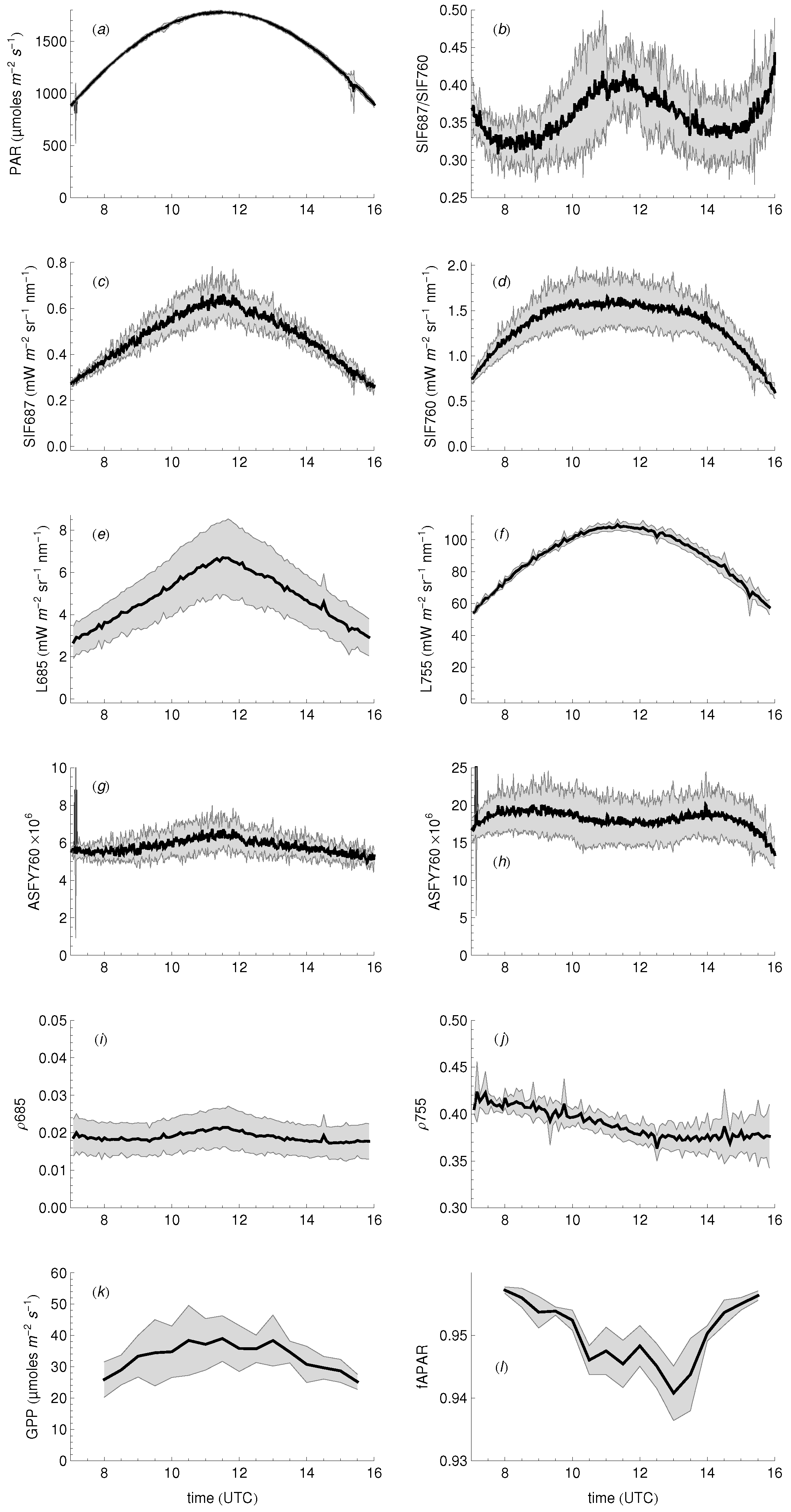
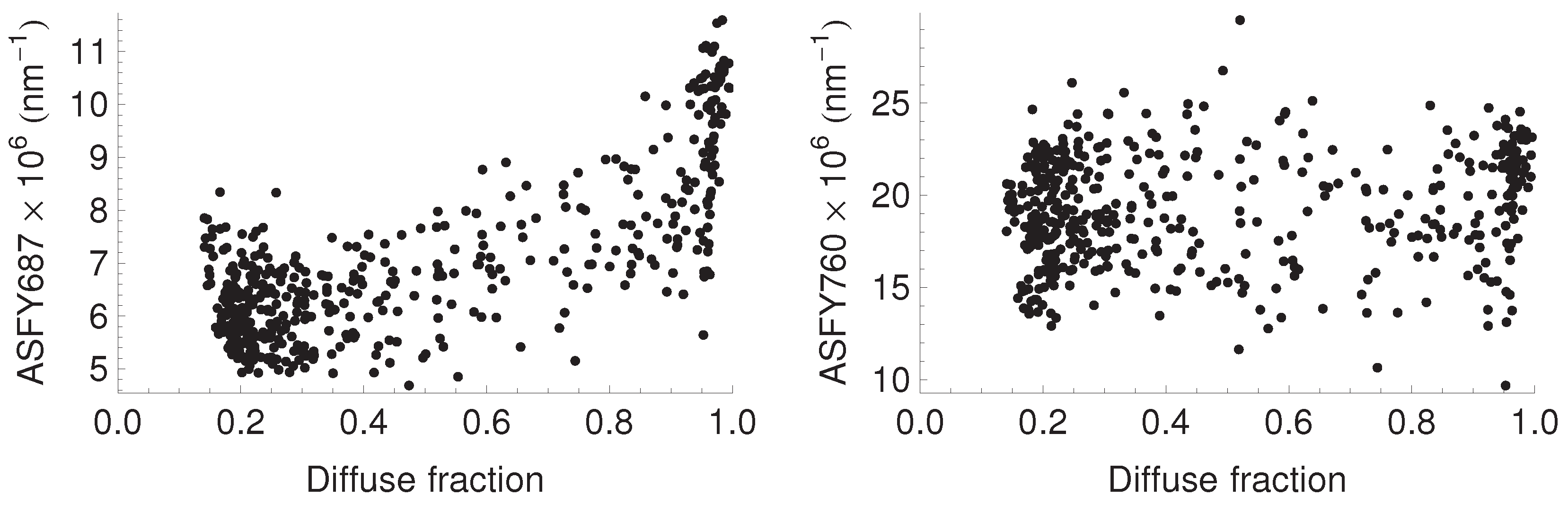
3.1. Daily Cycles of Fluorescence

Illumination conditions in terms of light intensity and incident angle present large variations during the time course of the day, which can impact light absorption and emission. Figure 3 shows mean diurnal patterns of top of canopy (TOC) red and far red radiances ($L685$, $L758$) and fluorescence signals (SIF687, SIF760, ASFY687, ASFY760) on sunny days , when the crop has reached a steady mature state (LAI = 6, see Table 1). PAR showed a typical variation close to a cosine law as a function of sun zenith angle (Figure 3a). Depending on emission wavelength, SIF exhibited different diurnal patterns: SIF687 showed an almost linear increase (decrease) with time before (after) solar noon, while SIF760 had a rather bell-shaped variation, reaching a steady state level around solar noon (Figure 3c,d). TOC radiances daily cycles were also wavelength-dependent (Figure 3e,f). An interesting result is that SIF and radiance patterns were quite similar for nearby wavelengths. At wavelengths strongly absorbed by chlorophyll (i.e., 687 nm for SIF and 685 nm for L), linear variations with time were observed. At non-absorbed wavelengths (i.e., 760 nm for SIF and 758 nm for L), the diurnal cycle showed a bell-shaped pattern similar to PAR. Differences in emission wavelengths were also reflected in the mean diurnal course of reflectances and ASFY (Figure 3g,h). ASFY687 reached its highest level around noon, while ASFY760 showed a small decrease compared to its morning value.

Diurnal variations of fAPAR—caused, for example, by leaf movements or by the complex interactions of varying incident angles with canopy structure—would affect ASFY diurnal pattern. To evaluate possible fAPAR effects on ASFY, we investigated the fAPAR time course by measuring the transmitted PAR and converted it into fAPAR using Equation (4). During the mature state of the crop, fAPAR showed only small variations, and a small decrease (<2%) could be observed in the middle of the day in clear sky conditions.

To better understand the origin of daily changes in ASFY, we compared SIF measurements with active fluorescence measurements performed at leaf level with the PAM-2000. Active measurements provide relative changes in fluorescence quantum yield if measurements are taken on the same leaf and if all experimental parameters are kept constant (e.g., measuring distance, measuring beam intensity). When comparing different leaves, changes in pigment content can result in an additional dispersion. Here we compared the PAM-2000 fluorescence level (Fs) between groups of leaves sampled in the morning and at noon on three different sunny days (

Table 2. Changes of fluorescence between morning ( 8:00 UTC) and noon ( 12:00 UTC) on sunny days. Fs: mean leaf fluorescence level measured with a PAM-2000; ${\mathrm{F}}^{\prime }$m: maximum fluorescence level of leaf upon a saturating pulse; ${\mathrm{\Phi }}_P$: leaf photochemical yield; number of samples as indicated; ASFY687 and ASFY760, apparent spectral fluorescence yield at $687$ and $760\mathrm{n}\mathrm{m}$ defined as the ratio between fluorescence radiance and incident PAR. Mean values between 8:00 and 8:30 (morning) and 12:00 and 12:30 (noon) are reported. Significance levels are indicated: n.s., * p < 0.05, ** p < 0.01, *** p < 0.001. The measuring distance on the leaf-clip was modified on DOY 149, so Fs and ${\mathrm{F}}^{\prime }$m measurements between DOYs 119–142 and DOYs 149–156 are not comparable.

Date	PAR ($\mathsf{\mu }\mathbf{mol}·{\mathbf{m}}^{-2}·{\mathbf{s}}^{-1}$)	Fs (a.u.)	${\mathrm{F}}^{\prime }$m (a.u.)	${\mathrm{\Phi }}_{\mathit{P}}$	ASFY687 (${\mathbf{nm}}^{-1}{10}^{-6}$)	ASFY760 (${\mathbf{nm}}^{-1}{10}^{-6}$)
2010/04/29 (DOY 119)		(n = 20)	(n = 20)	(n = 20)	(n = 30)	(n = 30)
morning	1159	0.377	0.6	0.367	0.37	1.14
Rel. var. noon/morning		−14% (***)	−25% (***)	−25% (***)	12% (***)	−3% (***)
2010/05/13 (DOY 133)		(n = 20)	(n = 20)	(n = 20)	(n = 30)	(n = 30)
morning	1230	0.344	0.498	0.302	0.318	1.13
Rel. var. noon/morning		−12% (*)	−16% (n.s.)	−12% (**)	11% (***)	−11% (***)
2010/05/17 (DOY 137)		(n = 19)	(n = 19)	(n = 19)	(n = 30)	(n = 30)
morning	1257	0.359	0.534	0.328	0.325	1.08
Rel. var. noon/morning		−15% (**)	−24% (***)	−25% (***)	15% (***)	−3% (*)
2010/05/20 (DOY 140)		(n = 20)	(n = 20)	(n = 20)	(n = 30)	(n = 30)
morning	1288	0.347	0.513	0.321	0.341	1.12
Rel. var. noon/morning		−17% (**)	−21% (n.s.)	−11% (***)	12% (***)	−16% (***)
2010/05/22 (DOY 142)		(n = 17)	(n = 17)	(n = 17)	(n = 30)	(n = 30)
morning	1189	0.322	0.77	0.557	0.287	0.88
Rel. var. noon/morning		−7% (n.s.)	−45% (***)	−47% (***)	4% (***)	−10% (***)
2010/05/29 (DOY 149)		(n = 32)	(n = 32)	(n = 32)	(n = 30)	(n = 30)
morning	1327	0.194	0.387	0.474	0.345	1.04
Rel. var. noon/morning		−10% (***)	−32% (***)	−30% (***)	6% (***)	−5% (**)
2010/06/02 (DOY 153)		(n = 30)	(n = 30)	(n = 30)	(n = 30)	(n = 30)
morning	1289	0.196	0.443	0.526	0.3.=35	0.952
Rel. var. noon/morning		−4% (n.s.)	−39% (***)	−45% (***)	27% (***)	−4% (**)
2010/06/04 (DOY 155)		(n = 30)	(n = 30)	(n = 30)	(n = 30)	(n = 30)
morning	1291	0.194	0.367	0.44	0.307	0.822
Rel. var. noon/morning		−13% (**)	−37% (***)	−44% (***)	8% (***)	−16% (***)
2010/06/05 (DOY 156)		(n = 20)	(n = 20)	(n = 20)	(n = 30)	(n = 30)
morning	1299	0.189	0.307	0.368	0.308	0.751
Rel. var. noon/morning		−20% (***)	−40% (***)	−52% (***)	14% (***)	−10% (***)

). The analysis was limited to sunny days to ensure repeatability in light intensity and quality between days. No significant differences in Fs were observed between groups taken at the same hour on different days. However, a slight but highly significant decrease (p < 0.01) was observed on six out of nine days when comparing noon groups to morning groups of leaves (−12% on average). A significant decrease between morning and noon was also observed on $F^{\prime }m$ and ${\mathrm{\Phi }}_P$ (−31% and −32% on average, respectively). The decrease in $F^{\prime }m$ shows that a significant amount of non photochemical quenching was accumulated at noon, which reduced the photochemical yield of photosystem II. Significant variations of ASFY687 and ASFY760 were also observed from Table 2 (+12% and −8.7% on average, respectively), but none correspond linearly to the amount of the decrease in photochemical yield.

During the day, surface irradiance can also present large changes in the fractions of direct and diffuse light. In order to evaluate the effect of light intensity and directionality on apparent yield, we compared the SIF–PAR relationship between clear sky and overcast days for different development stages of the crop (Figure 4). It was found that FRSIF was more responsive than red SIF to crop development, while it was less responsive to the diffuse fraction of PAR ( $f_{diffPAR}$). This point is further illustrated by Figure 5, where ASFY is plotted against $f_{diffPAR}$ for a mature crop only, to avoid LAI effects on ASFY. It clearly shows than ASFY687 increased with $f_{diffPAR}$, while ASFY760 showed almost no effect (see also

Table 3. Changes in mean ASFY upon sky conditions. Data taken from Figure 5.

	Clear Sky	Overcast
Diffuse fraction of PAR	≤0.2	≥0.9
n samples	221	93
Median PAR ($\mathsf{\mu }$mol$·$${\mathrm{m}}^{-2}$$·$${\mathrm{s}}^{-1}$)	1620	494
Median $ASFY687\times {10}^6$ ($\mathrm{n}{\mathrm{m}}^{-1}$)	6.1	9.3
Median $ASFY760\times {10}^6$ ($\mathrm{n}{\mathrm{m}}^{-1}$)	18.7	21.1

). The transition from clear to overcast sky has two main effects on irradiance: (i) a decrease in the PAR intensity; and (ii) a change in the incident angle distribution of the incoming light. We observed only a limited change of $Fs$ at leaf level when light level changed from 1500 to 500 $\mathsf{\mu }$mol$·$${\mathrm{m}}^{-2}$$·$${\mathrm{s}}^{-1}$ (+10%, see Section 3.4). This suggests that irradiance intensity is not the only factor acting on SIF, and that other factors such as the angular distribution of incoming PAR should also be considered in the relationship between SIF and PAR.

3.2. Seasonal Patterns of Fluorescence

Figure 6 gives an overview of the time course of the fluorescence signals during the whole measurements campaign, compared to NDVI, GPP, and fAPAR. NDVI increased at the beginning of the measurement period from a value of about 0.4–0.45, and reached a steady state level above 0.9 which lasted from DOY 100 to DOY 150, and then decreased slightly at the beginning of the senescent phase. It should be noted that during the steady state phase of NDVI, the crop still grew up, as can be seen from canopy height and biomass measurements (Figure 1; Table 1). During the measurement period, SIF687 varied from 0.2 to 0.8 mW$·$${\mathrm{m}}^{-2}·$${\mathrm{sr}}^{-1}·$${\mathrm{nm}}^{-1}$, while SIF760 varied from almost 0 to 2 mW$·$${\mathrm{m}}^{-2}·$${\mathrm{sr}}^{-1}·$${\mathrm{nm}}^{-1}$. SIF760 showed large variations in amplitude at the beginning of the measurement period during crop growth, even when NDVI reached a steady state level (Figure 6c,d). A strong decrease of SIF760 was also observed at the end of the experiment, associated with the senescent period and a decrease of leaves’ chlorophyll content (see Figure 1). Compared to SIF760 (Figure 6c), SIF687 (Figure 6b) showed more limited changes in intensity, despite crop growth and senescence. These contrasting evolution patterns between fluorescence bands are better evidenced by the time course of the emission ratio (Figure 6e). SIF687/SIF760 showed large variations during crop growth and senescence, and remained almost stable with low values between 0.25 and 0.6 during crop maturity. Normalization of SIF687 and SIF760 with PAR reduced diurnal and day-to-day variations, as can be seen from the seasonal patterns of ASFY687 and ASFY760 (Figure 6f,g). Again, it can also be observed that the two fluorescence bands exhibited very different patterns. ASFY687 showed less variations than ASFY760 during the different phases of the crop development (apart from some peaks associated with cloudy periods), while ASFY760 showed a regular increase from the beginning of the experiment and a strong decrease at senescence.

Figure 6 shows that fAPAR increased during the development stage (until DOY 120) and then remained stable from DOY 120 to DOY 154 at a high level (>0.93) until the beginning of senescence. During senescence, fAPAR decreased slightly, in association with a concomitant lowering of Chl content (Figure 1). fAPAR presented daily variations, which were up to 20% at the beginning of the growth phase (DOY < 110), but were greatly reduced as soon as fAPAR reached its highest values (≥2%).

At the seasonal scale, GPP presented a regular increase during crop growth from DOYs 60 to 120, and a strong decrease at senescence. The seasonal patterns of GPP and SIF760 were quite similar, but large differences were observed between the patterns of GPP and SIF687.

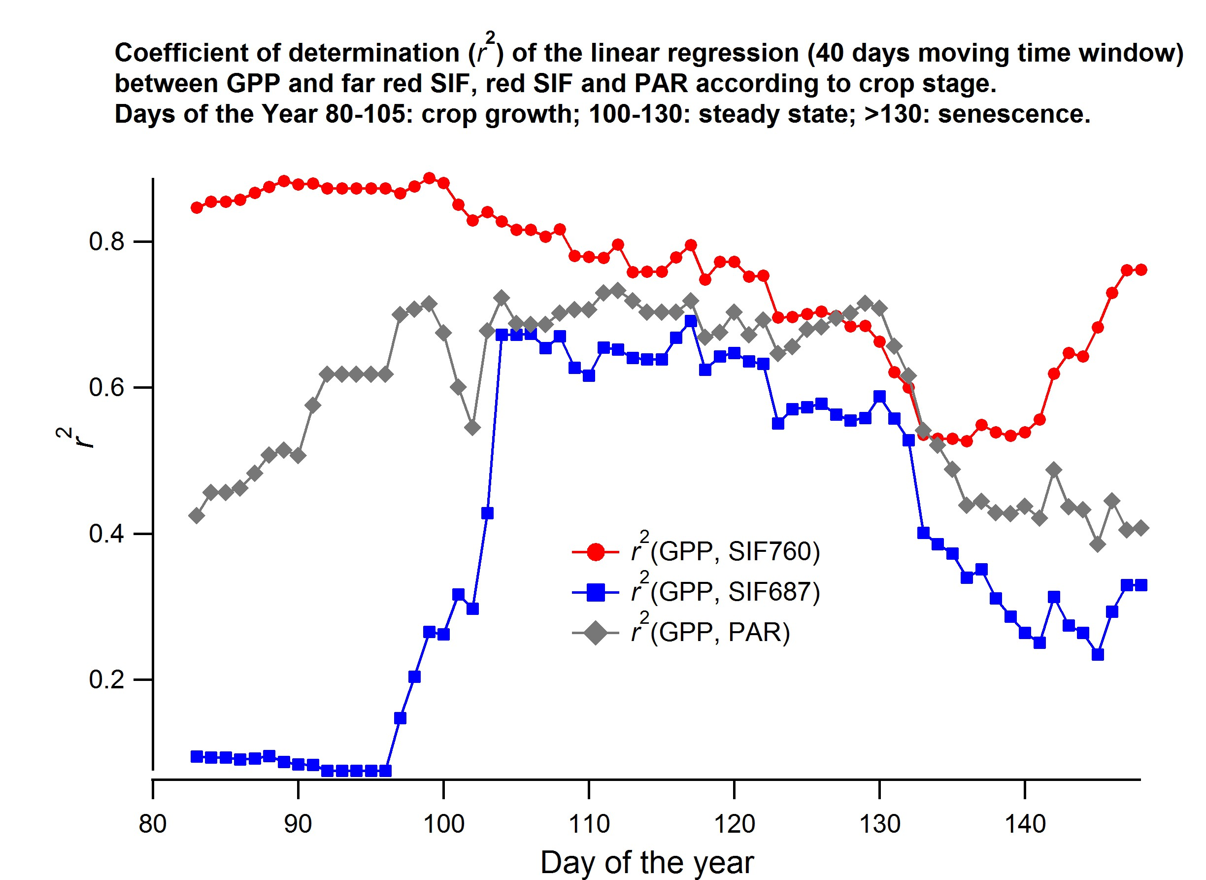
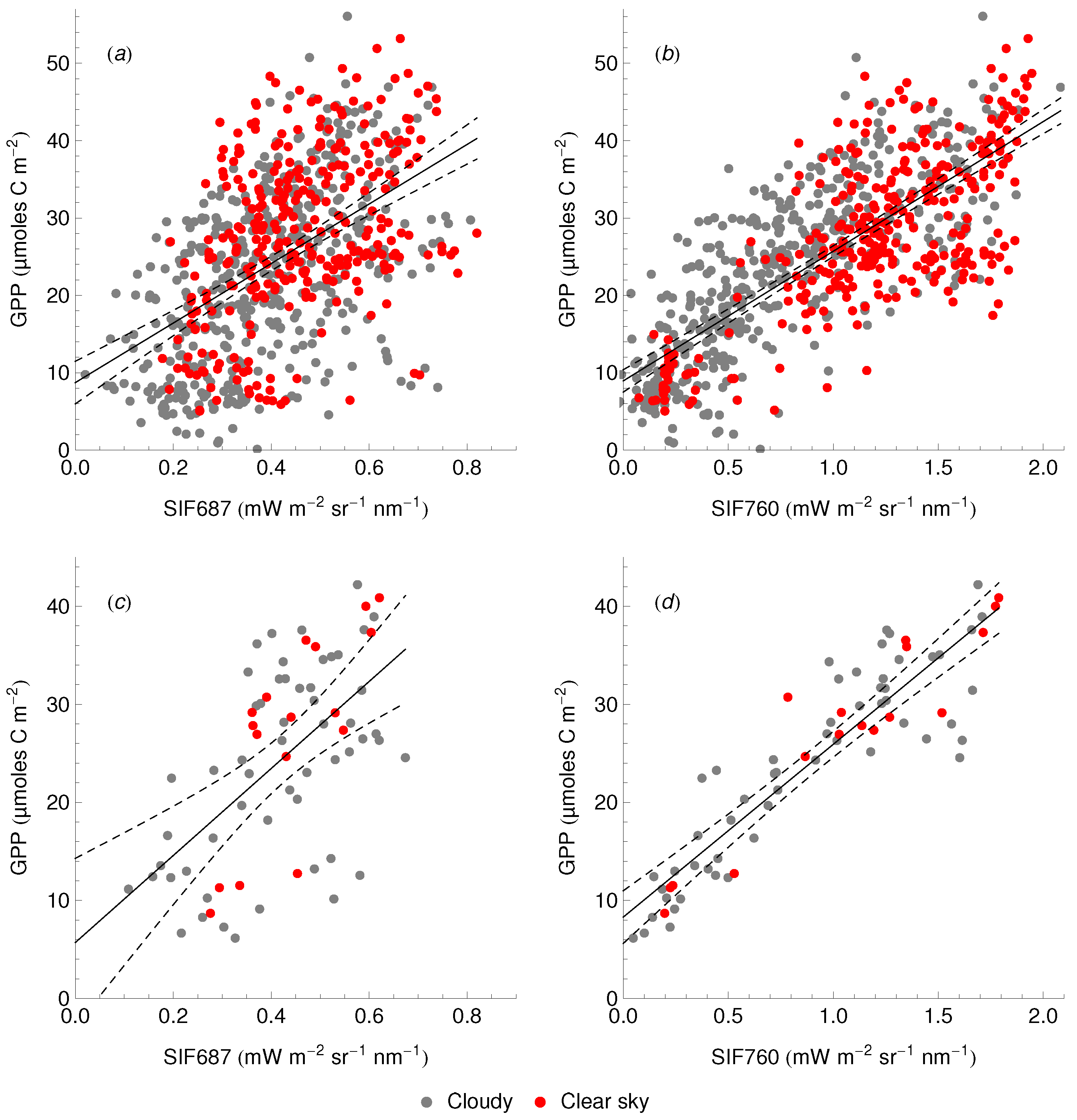
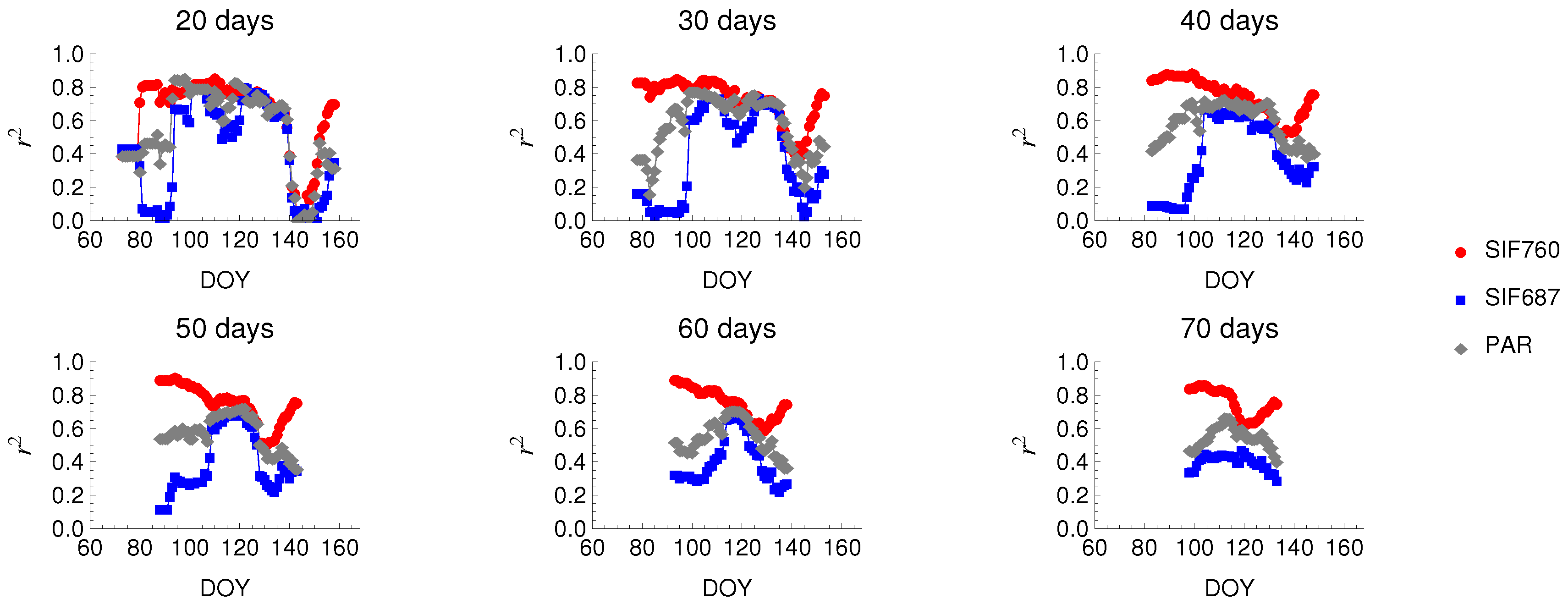
3.3. Relationship between SIF and GPP

The relationship between SIF and GPP was investigated by linear regression between the two variables upon different observational cases: (i) the emission wavelength (SIF687 vs. SIF760); (ii) the time scale of observation (vs. daily averages in the 8:00–15:30 UTC time period) (Figure 7); (iii) the diffuse fraction of PAR (clear sky vs. all sky conditions); and (iv) the time of observation. A significant relationship was found between half-hourly values of SIF760 and GPP ($r^2=0.58$, Figure 7b). Using daily instead of half-hourly averages significantly increased the coefficient of determination ($r^2=0.83$, Figure 7d), while the slope of the regression line did not change (17.6 ± 0.9 (1sd) (daily) instead of 17.2 ± 0.4 (1sd) $\mathsf{\mu }$moles C$·$${\mathrm{J}}^{-1}$$·$sr$·$$\mathsf{\mu }$m (half-hourly)). On the other hand, the relationship between half-hourly SIF687 and GPP was strongly reduced compared to SIF760 ($r^2=0.25$, Figure 7a). Using daily averages improved the relationship, but still gave a coefficient of determination ($r^2=0.34$) lower than the corresponding one for SIF760 (

Table 4. Statistics of the linear regression between SIF and GPP as a function of experimental conditions. Integration time: $30\min$, SIF and GPP are averaged over $30\min$; $6.5\mathrm{h}$, SIF and GPP are averaged between 8:00 and 15:30 UTC. Sky conditions: All, all measured points are included in the analysis; Clear sky, clear sky at the measuring time only; Clear sky during the whole day, only data from complete clear sky days are considered. p-value and t-statistics for the probability of the regression slope to be zero are indicated.

Integration Time	30 min	30 min	30 min	6.5 h	6.5 h
Sky Conditions	All	Clear Sky	Clear Sky during the Whole Day	All	Clear Sky during the Whole Day
data points	768	313	173	72	17
SIF687
$r^2$	0.25	0.16	0.33	0.34	0.58
p-value	<0.001	<0.001	<0.001	<0.001	<0.001
t-statistics	16.05	7.73	9.21	6.07	4.57
SIF760
$r^2$	0.58	0.52	0.61	0.83	0.88
p-value	<0.001	<0.001	<0.001	<0.001	<0.001
t-statistics	32.46	18.31	16.39	18.28	10.74

). The relationship between half-hourly SIF and GPP slightly weakened if we considered measurements under clear sky, except if we considered only measurements when the sky is clear during the full day (Table 4), where a slight increase of the coefficient of determination was observed. For daily-integrated measurements, limiting the observations to clear sky increased $r^2$ for both SIF687 and SIF760. A critical question in SIF remote sensing is the representativeness of single SIF measurements per day to describe carbon uptake over a long period of time [16,20]. Sun-synchronous satellites like GOSAT or FLEX can only acquire SIF once a day. For example, the orbit of FLEX allows a single measurement at 10:00 hours (local time descending node, LTDN), which varies slightly with latitude. We evaluated the relationship between SIF measured at a given time in the day and GPP. Two cases were considered for the integration time of GPP: (i) the instantaneous value, integrated over $30\min$ at the same time as the fluorescence measurement; and (ii) the daily integrated value between 8:00 and 15:30. Slight changes in the coefficient of determination were observed as a function of measurement time, with the strongest relationship occurring around noon (Figure 8). We therefore evaluated the relationship between SIF and GPP for SIF measurements at 12:00 according to different sky conditions: (i) clear and cloudy sky together; (ii) clear sky at the time of SIF measurement; (iii) clear sky during the entire day of measurement (

Table 5. Statistics of the linear regression between SIF averaged over $30\min$ between 12:00 and 12:30 UTC and GPP as a function of experimental conditions. GPP integration time: $30\min$, GPP is averaged over $30\min$ between 12:00 and 12:30 UTC; $6.5\mathrm{h}$, GPP is averaged between 8:00 and 15:30 UTC.Sky conditions: All, all measured points at 12:00 UTC are included in the analysis; Clear sky, clear sky at the measuring time only; Clear sky during the whole day, only data from completely clear sky days are considered. p-value and t-statistics for the probability of the regression slope to be zero are indicated.

GPP Integration Time	30 min	30 min	30 min	6.5 h	6.5 h	6.5 h
Sky Conditions	All	Clear Sky	Clear Sky during the Whole Day	All	Clear Sky	Clear Sky during the Whole Day
data points	52	19	10	64	25	15
SIF687
$r^2$	0.21	0.17	0.66	0.24	0.2	0.66
p-value	0.001	0.08	0.004	<0.001	0.02	<0.001
t-statistics	3.66	1.84	3.91	4.41	2.42	5.01
SIF760
$r^2$	0.56	0.56	0.75	0.76	0.78	0.93
p-value	<0.001	<0.001	0.001	<0.001	<0.001	<0.001
t-statistics	7.9	4.61	4.84	13.99	9.05	12.99

). It was found that mixing clear and cloudy sky conditions in the regression decreased the coefficient of determination. Additionally, the relationship decreased when we considered instantaneous values of GPP instead of daily integrated ones. The strongest relationship ($r^2=0.93$) was found for SIF760 when we only included data from clear sky days in the regression computation. This questions the potential of simple linear relationship based on SIF to estimate the fraction of carbon uptake that takes place during overcast days.

To evaluate the effect of the crop state on the relationship between GPP and SIF, we performed linear regressions on data from restricted time windows (Figure 9). We found noticeable changes in the coefficient of determination ($r^2$) when the regression period (20 to 70 days) was time shifted from the beginning of crop development to senescence. Figure 9 shows the result of linear regression between GPP and PAR. It can be seen that when a crop was under development, $r^2$ (GPP, SIF760) was much higher than $r^2$ (GPP, SIF687). As a crop entered into a steady state, the relationship between SIF760 and GPP slightly weakened, and the relationship between SIF687 and GPP became stronger. When a steady state was reached during the time window, $r^2$ (SIF760, GPP), and $r^2$ (SIF687, GPP) were close to each other, and close to $r^2$ (PAR, GPP). When the crop entered into the senescent phase, the difference between $r^2$ (SIF760, GPP) and $r^2$ (SIF687, GPP) increased again, and both $r^2$ (SIF687, GPP) and $r^2$ (PAR, GPP) decreased by almost the same amount. These results indicate that SIF687 does not «explain» GPP variance better than PAR does. Similar interpretations can be drawn when considering half-hourly data; however, with lower coefficients of determination (results not shown).

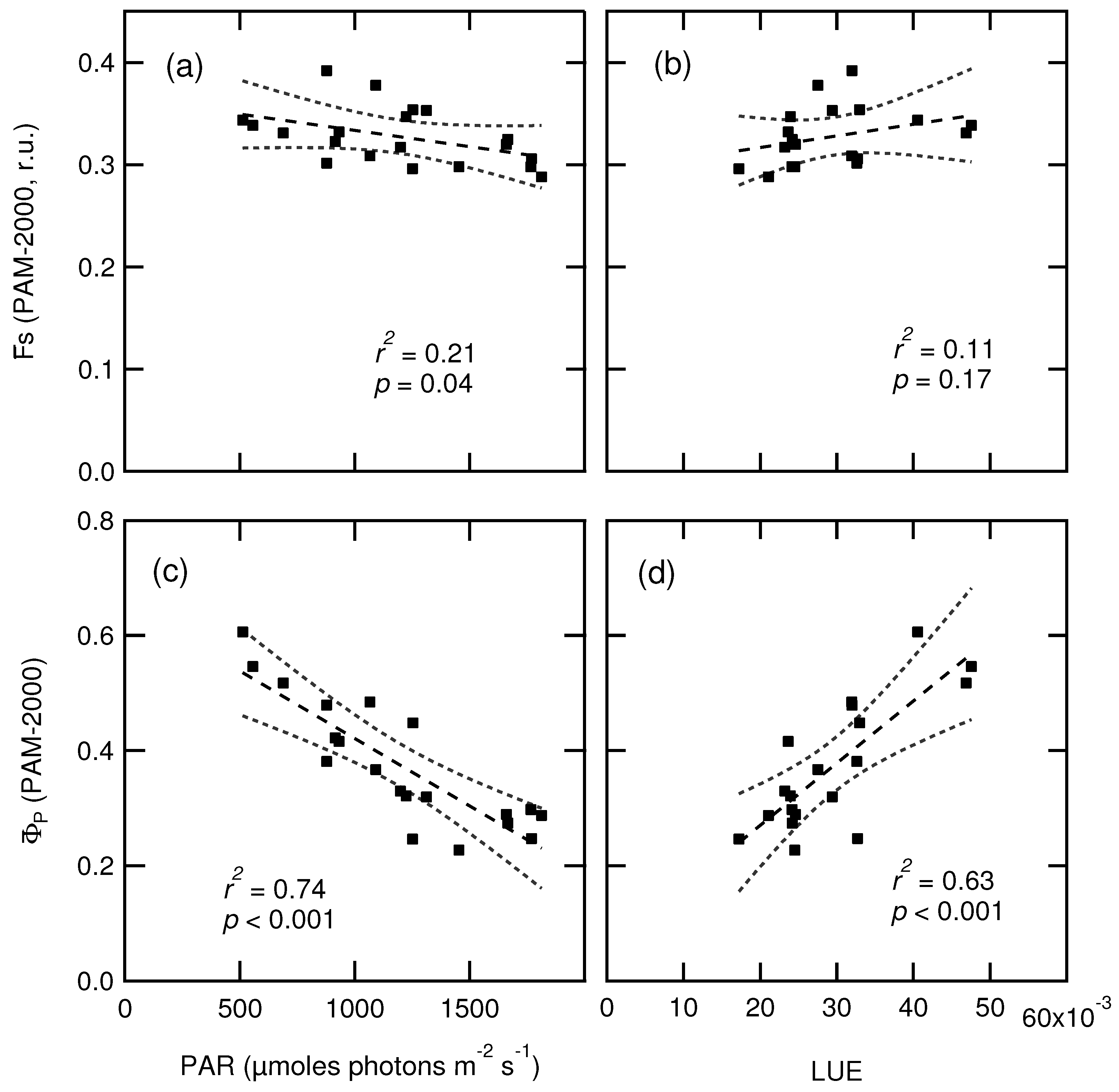
3.4. Relationship between Fluorescence Yield, Photochemistry, and Light Use Efficiency

We determined the leaf response to light level by measuring the fluorescence parameters ($Fs$, $\Delta F$/$F^{\prime }m$) on randomly selected leaves during the maturity stage of the crop (i.e., between DOY 118 and 143). During this period, incident PAR was almost totally absorbed by the canopy, and fAPAR remained almost constant at its maximum value with low diurnal variations (<2%, see Figure 6). In order to compare leaf measurements to EC data, leaf data obtained with the PAM-2000 at given times (8:30, 12:00, and 16:00) were averaged over the measured leaves to define a canopy-averaged photochemical yield ${\overline{\mathrm{\Phi }}}_P$ based on $\Delta F$/$F^{\prime }m$ and an averaged fluorescence yield $\overline{F}s$ (Figure 10). We found that $\overline{F}s$ was almost not responsive to light level in the range between 500–1800 $\mathsf{\mu }$mol$·$${\mathrm{m}}^{-2}$$·$${\mathrm{s}}^{-1}$, and no relationship between $\overline{F}s$ and LUE could be evidenced ($r^2=0.11$, p = 0.17). Similar results were found by investigating the relationship between LUE and the fluorescence yield defined at canopy level (SFY) (

Table 6. Statistics of the linear regression between half-hourly light use efficiency (LUE) and spectral fluorescence yield (SFY) for different crop stages and sky conditions. The analysis includes data between DOY 97 and 167 when fAPAR data is available.

Crop Stages	All	Without Senescence	Without Senescence
Sky Conditions	All	All	Clear Sky
Data points	665	531	253
687 nm
$r^2$	0.11	0.16	0.007
p-value	<0.0001	<0.0001	0.19
760 nm
$r^2$	0.10	0.006	0.05
p-value	<0.0001	0.06	0.0002

). Although statistically significant relationships could be found in some cases according to the p-values, $r^2$ values stayed low, which means that SFY can only «explain» a minor part of LUE variation in this case. This contrasts with the relationships found between ${\overline{\mathrm{\Phi }}}_P$ and PAR and between ${\overline{\mathrm{\Phi }}}_P$ and LUE, where an almost proportional relationship was found between ${\overline{\mathrm{\Phi }}}_P$ and LUE (${\overline{\mathrm{\Phi }}}_P=(0.053\pm 0.18)+(10.8\pm 5.8)LUE$, $r^2=0.63$).

4. Discussion

4.1. Fluorescence Retrieval in the O₂-A and O₂-B Bands

SIF was retrieved from canopy radiance by using the principle of in-filling of oxygen absorption bands in the radiance spectrum by fluorescence emission. Using this principle, the band profile of the vegetation radiance spectrum was compared to the corresponding profile of a reference spectrum acquired on a white flat panel. In the FLD (Fraunhofer Line Discrimination) method initially introduced by Plascyk [7], substantial errors can result from the spectral variation of reflectance over the absorption band [35,46,47]. Improved retrieval methods were designed to account for the reflectance and fluorescence spectral shapes in the absorption bands region, such as 3FLD [48], iFLD [46], cFLD [13,49], SFM (Spectral Fitting Method) [11,47], or SVD-based (Singular Vector Decomposition) [50]. In the method used in this study and formerly introduced in [32], three or four spectral channels are used to sample radiances in order to better take into account the shape of the reflectance spectrum of the vegetation. Near the O₂-A band, reflectance varies almost linearly and, therefore, three channels are used (3FLD). In the O₂-B band, four channels are required to characterize the curvature of reflectance (4FLD). The performance of this method has already been tested against direct measurements of leaf fluorescence and same values of emission ratio were found within the experimental error [35].

In Appendix A, we evaluated this method on simulated radiance spectra with known reflectance and known fluorescence levels. In the O₂-A band, and using three channels for the retrieval, the mean difference over the simulated database between the retrieved fluorescence and the true value (${\overline{SIF}}_{bias}$) is 0.015 $\mathsf{\mu }$mol$·$${\mathrm{m}}^{-2}·$${\mathrm{sr}}^{-1}·$${\mathrm{nm}}^{-1}$ under an irradiance of 1400 $\mathsf{\mu }$mol$·$${\mathrm{m}}^{-2}$$·$${\mathrm{s}}^{-1}$. It represents about 1.2% of the experimental level observed on the fully developed crop (median value of SIF760 is 1.3 $\mathsf{\mu }$mol$·$${\mathrm{m}}^{-2}·$${\mathrm{sr}}^{-1}·$${\mathrm{nm}}^{-1}$ under the same irradiance). In the total error budget, the ${\overline{SIF}}_{RMSE}$—which represents the dispersion of the error over the simulated cases of the database used in Appendix A—should also be considered. We cannot certify that the whole database of the simulated cases corresponds exactly to the experimental cases that we encountered in our study, even if we tried to use input parameters in SCOPE simulations that are as close as possible to the real ones. However, we can consider that ${\overline{SIF}}_{bias}\pm {\overline{SIF}}_{RMSE}$ will give a good estimate of the error in most cases. Reported to a level of 1.3 $\mathsf{\mu }$mol$·$${\mathrm{m}}^{-2}·$${\mathrm{sr}}^{-1}·$${\mathrm{nm}}^{-1}$ for the median value of SIF760, this error will not exceed 3%.

In the O₂-B band, the corresponding retrieved bias is -0.038 $\mathsf{\mu }$mol$·$${\mathrm{m}}^{-2}·$${\mathrm{sr}}^{-1}·$${\mathrm{nm}}^{-1}$ with four channels and 0.13 $\mathsf{\mu }$mol$·$${\mathrm{m}}^{-2}·$${\mathrm{sr}}^{-1}·$${\mathrm{nm}}^{-1}$ with three channels. Therefore, SIF687 is on the average underestimated by the 4FLD method, while it is largely overestimated by the 3FLD method. Given the lower value of SIF687 compared to SIF760, this will lead to larger relative errors on SIF687. Reported to the median value of SIF687 retrievals of the experimental dataset at the same irradiance level (0.5 $\mathsf{\mu }$mol$·$${\mathrm{m}}^{-2}·$${\mathrm{sr}}^{-1}·$${\mathrm{nm}}^{-1}$ at 1400 $\mathsf{\mu }$mol$·$${\mathrm{m}}^{-2}$$·$${\mathrm{s}}^{-1}$), an averaged bias of 6% is expected. However, the $RMSE$ is also greater for retrieval in the O₂-B (0.06 $\mathsf{\mu }$mol$·$${\mathrm{m}}^{-2}·$${\mathrm{sr}}^{-1}·$${\mathrm{nm}}^{-1}$). If we consider the $RMSE$ in the error budget, we have to acknowledge that SIF687 can be underestimated in some cases by almost 20%.

4.2. Diurnal Cycles and Short Term Changes in Fluorescence

Leaves experience important light changes during the day or from day to day, due to change in sun elevation, cloud cover, or occultation by other leaves. If considering other things to be equal, SIF scales linearly with irradiance. To better assess the effect of other factors on SIF, we normalized it by PAR to define an apparent yield fluorescence yield at top of canopy (ASFY687 and ASFY760). Light-induced changes on SIF were evaluated on repetitive clear sky days. It was found that ASFY687 and ASFY760 slightly change during the day (by about 20% and 10%, respectively, Figure 3). Additional differences between red and far red fluorescence were revealed when comparing diurnal cycles of SIF687 with SIF760, as well as ASFY687 with ASFY760, and when investigating the fluorescence ratio SIF687/SIF760 (Figure 3). There is a possibility that at least a part of these differences could be due to fluorescence retrieval errors. SIF retrievals on simulated radiances spectra have demonstrated a RMSE of 0.06 $\mathsf{\mu }$mol$·$${\mathrm{m}}^{-2}·$${\mathrm{sr}}^{-1}·$${\mathrm{nm}}^{-1}$ under a PAR of 1400 $\mathsf{\mu }$mol$·$${\mathrm{m}}^{-2}$$·$${\mathrm{s}}^{-1}$, which represents about 10–15% of SIF687. These simulation results also showed that the 4FLD algorithm tends to underestimate SIF by about 0.038 $\mathsf{\mu }$mol$·$${\mathrm{m}}^{-2}·$${\mathrm{sr}}^{-1}·$${\mathrm{nm}}^{-1}$ on average. Hence, an underestimation of SIF687 in the morning and in the evening due to retrieval errors could be a possible cause of the observed difference between SIF687 and SIF760. Another source of errors which is not accounted for by conventional retrieval algorithms (nFLD or SFM) is the effect of bidirectional reflectance of canopies associated with spectral anisotropy of sky radiance. Some authors pointed out that bidirectional properties of canopy reflectance may induce errors in SIF retrieval, depending on the difference between reflectances under diffuse and direct lights on one hand, and on the fractions of diffuse and direct irradiances on the other hand [51,52,53]. Because of different optical pathways in the atmosphere, direct and diffuse irradiances show different spectral patterns in the oxygen bands. Specifically, the depth of the band (defined as the ratio between the irradiance at the edge of the band and the irradiance at the bottom of the band) is generally deeper for diffuse than for direct irradiance, because of the larger optical pathway of diffuse light [6]. In addition, the reflectivity of the canopy could differ between direct and diffuse light because of its complex interaction with incident light and angularly-dependent leaf surface polarization. This would result in differences between the radiance spectra of the reference panel and vegetation unrelated to fluorescence emission, which are a possible source of error in the retrieved SIF signal [54]. Here, we cannot exclude a contribution of bidirectional reflectance to the observed differences in the dynamics of SIF687 and SIF760.

However, similar differences in the diurnal patterns can be observed between TOC radiances at wavelengths close to the SIF bands ($L685$ and $L755$). Unlike SIF, radiances are not subject to retrieval errors. This suggests a common origin for the observed differences in the diurnal patterns between SIF687 and SIF760, and between $L685$ and $L755$. A possible origin is the difference in the radiative transfer within the canopy layers of the emitted/reflected–transmitted light depending on wavelength, as red light is strongly re-absorbed by chlorophyll and far red is not. Such a pattern with an almost linear increase (and decrease) of SIF687 has been found on pine [10], but not on sorghum [9], which is in line with a possible effect of canopy architecture in relation with radiative transfer. Additional experiments, using for example active measurements of fluorescence and/or simulations with a canopy fluorescence model like SCOPE are necessary to evaluate this hypothesis. Other phenomena (like leaf movements) could also play a role in the diurnal cycle of SIF by modifying radiative transfer inside the canopy along the day.

On the other hand, physiological effects should also be taken into account to interpret diurnal cycles of SIF. Red SIF originates solely from PSII, whose emission varies with photochemical and non-photochemical quenching (PQ and NPQ, respectively), while far red SIF additionally includes a constant PSI component. In this view, parallel changes of SIF687 and SIF760 with physiology (i.e., fluorescence quenching) are expected, with a larger amplitude for SIF687. Physiological effects can be accounted for by active fluorescence measurements at leaf level. In this study, $F_s$, $F_m^{\prime }$, and ${\mathrm{\Phi }}_P$ were assessed on leaves randomly distributed in the canopy. These measurements showed a parallel decrease of $F_m^{\prime }$ and ${\mathrm{\Phi }}_P$ at noon, which indicates an accumulation of non-photochemical quenching. A slight but statistically significant decrease of $F_s$ was also observed. This decrease of $F_s$ is in good agreement with the observed change in ASFY760, but not with the increase of ASFY687. This means that physiological effects are masked or tightly coupled to other types of effects, such as radiative transfer effects induced by changes in the illumination geometry. We should point out that the approach used here to compare active and passive measurements is oversimplified, as it does not take into account the possible interaction between the distribution of physiological effects on fluorescence (e.g., different fluorescence yields between shaded and sunlit leaves, or between upper and lower leaves) and the radiative transfer of incident and emitted light in the canopy. A more sophisticated approach based on a radiative transfer modelling would be necessary to take these effects into account. A good agreement between PAM fluorescence and far red SIF has already been observed on a maize canopy after treatment with the herbicide DCMU [6]. Additionally, significant positive correlations between $Fs$ measured at leaf level and SIF760 extracted from pure crown pixels obtained by airborne imaging spectrometer have been observed on olive and peach orchards [55] and vineyard [56].

Short term changes include changes in the distribution function of incoming light incident angles due to aerosol content or cloud cover. It can be assessed by the relationship between apparent fluorescence yield and the diffuse PAR fraction ($F_{diffPAR}$). Here, we observe an increase of the median value of ASFY687 by about 50% when comparing overcast sky conditions ($f_{diffPAR}\ge 0.9$) to clear sky conditions ($f_{diffPAR}\le 0.3$), while the corresponding change in ASFY760 does not exceed 13%. Overcast is associated with a large decrease of PAR (from about $1600$ to 500 $\mathsf{\mu }$mol$·$${\mathrm{m}}^{-2}$$·$${\mathrm{s}}^{-1}$ in this case), which induces changes in the rate of PQ and NPQ, but we did not observe such high changes at leaf level in $Fs$. Therefore, we infer that non-physiological effects are playing a role in ASFY687. They might be linked to bidirectional reflectance (BR) effects associated with a spectral anisotropy of irradiance that are not taken into account in the SIF retrieval algorithm and/or to changes in radiative transfer through the canopy in link with the illumination geometry.

4.3. Seasonal Changes in Fluorescence

Long term observations (i.e., at the seasonal time scale) are characterized by large changes in canopy structure (height, biomass, LAI) and by more stable or repetitive conditions of illumination, if we do not consider cloudy periods. Here, we observed very different seasonal patterns between red and far red SIF. Specifically, crop development and senescence are associated with large changes in ASFY760, which are not seen in ASFY687 (Figure 6f,g). This is in contrast with recent results obtained on corn crops [23]. These authors observed almost similar trends of red and far red SIF over four seasonal cycles. A possible effect of canopy structure on the differences between red and far red SIF cannot be ruled out, as wheat and corn have different canopy architectures. However, in their study, a different instrumental configuration and retrieval algorithm were used, as they measured only three channels in the O₂-B bands with a spectral resolution of $1.5\mathrm{n}\mathrm{m}$. In this case, the curvature of the canopy reflectance spectrum in the O₂-B region cannot be taken into account, which would induce retrieval errors. The differences in seasonal variations of SIF can be interpreted in terms of different absorption foliage properties between red and far red light. When new leaves emerge and LAI increases, red fluorescence emitted by underneath leaves is blocked by the new layer, limiting the total red fluorescence that escapes the canopy. This is not the case of far red fluorescence, which is scattered by leaves and have a much higher probability to escape from the canopy. In our case, these structure-dependent effects on SIF are observed on wheat, which presents an erectophile leaf angle distribution [38,39]. Further studies associated to a relevant modeling scheme are needed to better characterize re-absorption effects (linked to the escape factor $\tau \left(\lambda \right)$) and bidirectional reflectance effects in the diurnal dynamic of SIF.

4.4. The SIF–GPP Relationship

In our study, a significant correlation between SIF and GPP was observed, as in other studies [16,19,20,22,23]. We observed large variations in the coefficient of determination ($r^2$) of the linear regression between SIF and GPP, according to emission wavelength, time scale of observation, sky conditions, or phenological stage. The weakest relationship ($r^2<0.1$) was observed for SIF687, and the strongest ($r^2>0.9$) for SIF760. In the regression between SIF687 and GPP, the lowest values of $r^2$ were obtained during the development phase. This supports the view that—unlike SIF760—SIF687 appears to be a poor indicator of crop development, and it is also not suitable to track GPP changes induced by an increase or decrease in photosynthetic biomass. In all cases, $r^2$ values for SIF687 were lower than the corresponding value for SIF760. A low correlation between red SIF and GPP has also been found on maize in another study [23]. On leaves, a positive correlation was observed between fluorescence and carbon assimilation, which has been attributed to increased levels of non-photochemical quenching (NPQ) that dissipates excess energy at the photosystem II level [57]. As NPQ acts on PSII fluorescence, one may expect a better positive correlation between photosynthesis and red fluorescence—where PSII preferentially emits—than with far red fluorescence, which is enriched by a constant PSI fluorescence contribution. This is not the case in our data, which suggests that other mechanisms not linked to fluorescence quenchings control the relationship between SIF and GPP.

The highest correlation with GPP was found for SIF760 during canopy structure changes (e.g., during development between DOYs 60–120 or senescence after DOY 150). These time periods are characterized by rapid changes in the amount of photosynthetic biomass and the fraction of APAR. SIF760—unlike SIF687 or reflectance indices like NDVI—has the capability to track these seasonal changes with a high dynamic range, which is supported by data from Figure 6. This parallel change between SIF760 and photosynthetic biomass (and hence between SIF760 and APAR) has been previously suggested by Moya et al. [58], and was further supported by subsequent studies on pine [10], rice [22], and sorghum [9].

In this study, we found that the stationary fluorescence yield as estimated by active measurements at leaf level was not linked to LUE (Figure 10). We also found small variations of ASFY for a given state of the crop, which are much lower than LUE variations. On the other hand, the photochemical yield of PSII (${\overline{\mathrm{\Phi }}}_P$) and LUE appear to be strongly linearly correlated ($r^2=0.63,p<0.001$). Positive correlation between the SIF normalized by APAR (${\mathrm{SIF}}^{yield}$) and LUE have been found in other studies [23,29,59], although no proportional relationship was evidenced. This contradicts theoretical claims that assume that under strong illumination, the ratio of LUE to fluorescence yield remains relatively constant [21,60,61]. In any case, the lack of a proportional relationship between ${\mathrm{SIF}}^{yield}$ (i.e., ASFY/fAPAR or SIF/APAR) and LUE will induce a lowering of the $r^2$ coefficient when large variations of LUE occur.

In our study, we found a high sensitivity of SIF760 to chlorophyll-driven changes in GPP (Figure 6) and a low sensitivity of fluorescence yield ($\overline{F}s$) to changes in LUE (Figure 10). These results suggest that the strong empirical correlation found between FRSIF and GPP in this study and in other previous ones [16,20,22] is most likely driven by the close link between FRSIF and APAR rather than by the recognized link between fluorescence yield and photosynthetic efficiency. This indicates that FRSIF has limited capabilities to capture both chlorophyll content and quenching-induced changes in GPP, contrary to what is suggested in [20]. Multiple-variable strategies should be considered instead of a single-variable relationship. In this perspective, the photochemical reflectance index (PRI) can bring complementary information to derive the photosynthetic efficiency component of GPP [62,63]. In another perspective, the ratio between GPP and FRSIF (SIF760 in our case) can be used to assess the primary productivity efficiency. Data from Figure 7 shows that the slope of the regression line between GPP and SIF760 does not change with integration time (0.5 $\mathrm{h}$ or 6 $\mathrm{h}$). Here, it is found to be 17.6 ± 0.9 $\mathsf{\mu }$molC$·$${\mathrm{J}}^{-1}$$·$sr$·$$\mathsf{\mu }$m. After correction for the emission wavelength and adequately scaled for the GPP integration time, this value is within the range of the slopes of the linear models derived from space measurements with the TANSO instrument on board the GOSAT satellite [16,17,19], and comparable to the coefficient of the SIF-based GPP model for crops and grasslands derived from GOME-2 data (14.9 $\mathsf{\mu }$molC$·$${\mathrm{J}}^{-1}$$·$sr$·$$\mathsf{\mu }$m) [20]. It should be noted that these results were obtained despite the differences in: (i) the measuring technique (atmospheric oxygen band vs. Fraunhofer lines in the case of GOSAT); (ii) the footprint (4 ${\mathrm{m}}^2$ vs. 4° × 4°, or vs. 40 × 80 ${\mathrm{km}}^2$); (iii) the time scale (daily measurement vs. monthly averages); and (iv) the measuring distance (21 $\mathrm{m}$ vs. around 800 $\mathrm{k}$$\mathrm{m}$). Hence, the GPP–FRSIF relationship appears to be robust across methods, or time and spatial scales. This study confirms the use of ground-based studies to provide data for the development of SIF-based GPP models that could be used in the future at larger scales. However, further work is needed to investigate the variability of the GPP–FRSIF relationship among species and biomes, as well as its response to stress conditions.

5. Conclusions

In this paper, we investigated diurnal and seasonal dynamics of red and far red SIF over a full seasonal cycle on a wheat crop, and its relationship with carbon uptake assessed by eddy covariance techniques. Using active techniques, fluorescence and PSII photochemical yield were measured at leaf level and compared to TOC measurements. We found a low diurnal variability of the apparent fluorescence yield (ASFY) during clear sky days, although differences between red and far red SIF can be observed. Diurnal changes in ASFY760 are in agreement with active leaf measurements of the mean stationary fluorescence level $\overline{F}s$, while ASFY687 shows variations in opposite direction. Under cloudy sky, ASFY687 shows a noticeable increase, while ASFY760 does not change. On the seasonal time scale, far red SIF appears to indicate better canopy growth and changes in chlorophyll content during senescence than red SIF. We observed a strong linear relationship between far red SIF and GPP ($r^2$ ranging from $0.5$ to >0.9, p < 0.001). This relationship is stronger during the phase of canopy growth or changes in chlorophyll content. It is also stronger when only clear sky days are considered, and for daily integrated values compared to $30\min$ integrated ones. In all cases, the relationship between red SIF and GPP is weaker than the corresponding one between far red SIF and GPP. The red SIF–GPP relationship is also the weakest during canopy growth. When canopy is in a steady phenophase, SIG687 and SIF760 are almost as effective as incoming PAR in predicting GPP. In view of these results, the use of SIF to directly assess GPP with simple linear regression presents some limitations. We showed that the relationship between SIF and GPP is highly variable depending on the emission wavelength, the time scale of observation, and/or the phenological stage of the crop. A part of the loss in correlation can be attributed to re-absorption effects, as for RSIF, which poorly correlates with GPP in all cases. Another part can be attributed to the non-proportional relationship between $Fyield$ and LUE that was evidenced in our study by active fluorescence measurements. Our results suggest that using simple linear relationships to infer GPP from SIF can only be applied in specific cases: with FRSIF, a high dynamic range of green biomass and a low variation range of LUE. In other cases, approaches using more sophisticated algorithms that exploit the full range of the available optical information, including RSIF, PRI (Photochemical Reflectance Index) [64,65], and reflectance should be considered. It is important to note that these results have been obtained on a single wheat crop over a single season. Further experiments must be conducted over multiple seasons on different crops and species before drawing general conclusions on the relationship between SIF and GPP.

References

1. Lichtenthaler, H.K.; Rinderle, U. The role of chlorophyll fluorescence in the detection of stress conditions in plants. CRC Crit. Rev. Anal. Chem. 1988, 19, 29–85. [Google Scholar] [CrossRef]
2. Maxwell, K.; Johnson, G.N. Chlorophyll fluorescence—A practical guide. J. Exp. Bot. 2000, 51, 659–668. [Google Scholar] [CrossRef] [PubMed]
3. Papageorgiou, G.; Govindjee. Chlorophyll a Fluorescence. A Signature of Photosynthesis; Advances in Photosynthesis and Respiration; Springer: Dordrecht, The Netherlands, 2004. [Google Scholar]
4. Baker, N.R. Chlorophyll fluorescence: A probe of photosynthesis in vivo. Annu. Rev. Plant Biol. 2008, 59, 89–113. [Google Scholar] [CrossRef] [PubMed]
5. Moya, I.; Guyot, G.; Goulas, Y. Remotely sensed blue and red fluorescence emission for monitoring vegetation. ISPRS J. Photogram. Remote Sens. 1992, 47, 205–231. [Google Scholar] [CrossRef]
6. Moya, I.; Camenen, L.; Evain, S.; Goulas, Y.; Cerovic, Z.G.; Latouche, G.; Flexas, J.; Ounis, A. A new instrument for passive remote sensing: 1. Measurements of sunlight-induced chlorophyll fluorescence. Remote Sens. Environ. 2004, 91, 186–197. [Google Scholar] [CrossRef]
7. Plascyk, J. The MK II Fraunhofer line discriminator (FLD-II) for airborne and orbital remote sensing of solar-stimulated luminescence. Opt. Eng. 1975, 14, 339–346. [Google Scholar] [CrossRef]
8. Meroni, M.; Rossini, M.; Guanter, L.; Alonso, L.; Rascher, U.; Colombo, R.; Moreno, J. Remote sensing of solar-induced chlorophyll fluorescence: Review of methods and applications. Remote Sens. Environ. 2009, 113, 2037–2051. [Google Scholar] [CrossRef]
9. Daumard, F.; Goulas, Y.; Champagne, S.; Fournier, A.; Ounis, A.; Olioso, A.; Moya, I. Continuous monitoring of canopy level sun-induced chlorophyll fluorescence during the growth of a sorghum field. IEEE Trans. Geosci. Remote Sens. 2012, 50, 4292–4300. [Google Scholar] [CrossRef]
10. Louis, J.; Ounis, A.; Ducruet, J.M.; Evain, S.; Laurila, T.; Thum, T.; Aurela, M.; Wingsle, G.; Alonso, L.; Pedros, R.; et al. Remote sensing of sunlight-induced chlorophyll fluorescence and reflectance of Scots pine in the boreal forest during spring recovery. Remote Sens. Environ. 2005, 96, 37–48. [Google Scholar] [CrossRef]
11. Meroni, M.; Colombo, R. Leaf level detection of solar induced chlorophyll fluorescence by means of a subnanometer resolution spectroradiometer. Remote Sens. Environ. 2006, 103, 438–448. [Google Scholar] [CrossRef]
12. Moya, I.; Camenen, L.; Latouche, G.; Mauxion, C.; Evain, S.; Cerovic, Z. An instrument for the measurement of sunlight excited plant fluorescence. In XIth International Congress Photosynthesis; Garab, G., Ed.; Kluwer Academic Publishers: Dordrecht, The Netherlands, 1999; Volume V, pp. 4265–4370. [Google Scholar]
13. Moya, I.; Daumard, F.; Moise, N.; Ounis, A.; Goulas, Y. First airborne multiwavelength passive chlorophyll fluorescence measurements over La Mancha (Spain) fields. In Proceedings of the 2nd International Symposium on Recent Advances in Quantitative Remote Sensing: RAQRS’II, Torrent, Spain, 25–29 September 2006.
14. Rascher, U.; Agati, G.; Alonso, L.; Cecchi, G.; Champagne, S.; Colombo, R.; Damm, A.; Daumard, F.; de Miguel, E.; Fernandez, G.; et al. CEFLES2: The remote sensing component to quantify photosynthetic efficiency from the leaf to the region by measuring sun-induced fluorescence in the oxygen absorption bands. Biogeosciences 2009, 6, 1181–1198. [Google Scholar] [CrossRef] [Green Version]
15. Zarco-Tejada, P.J.; González-Dugo, V.; Berni, J.A.J. Fluorescence, temperature and narrow-band indices acquired from a UAV platform for water stress detection using a micro-hyperspectral imager and a thermal camera. Remote Sens. Environ. 2012, 117, 322–337. [Google Scholar] [CrossRef]
16. Frankenberg, C.; Fisher, J.B.; Worden, J.; Badgley, G.; Saatchi, S.S.; Lee, J.E.; Toon, G.C.; Butz, A.; Jung, M.; Kuze, A.; et al. New global observations of the terrestrial carbon cycle from GOSAT: Patterns of plant fluorescence with gross primary productivity. Geophys. Res. Lett. 2011, 38, L17706. [Google Scholar] [CrossRef]
17. Joiner, J.; Yoshida, Y.; Vasilkov, A.P.; Corp, L.A.; Middleton, E.M. First observations of global and seasonal terrestrial chlorophyll fluorescence from space. Biogeosciences 2011, 8, 637–651. [Google Scholar] [CrossRef] [Green Version]
18. European Space Agency (ESA). Report for Mission Selection: FLEX; Technical Report ESA SP-1330/2; European Space Agency: Paris, France, 2015; p. 197. [Google Scholar]
19. Guanter, L.; Frankenberg, C.; Dudhia, A.; Lewis, P.E.; Gómez-Dans, J.; Kuze, A.; Suto, H.; Grainger, R.G. Retrieval and global assessment of terrestrial chlorophyll fluorescence from GOSAT space measurements. Remote Sens. Environ. 2012, 121, 236–251. [Google Scholar] [CrossRef]
20. Guanter, L.; Zhang, Y.; Jung, M.; Joiner, J.; Voigt, M.; Berry, J.A.; Frankenberg, C.; Huete, A.R.; Zarco-Tejada, P.; Lee, J.E.; et al. Global and time-resolved monitoring of crop photosynthesis with chlorophyll fluorescence. Proc. Natl. Acad. Sci. USA 2014, 111, E1327–E1333. [Google Scholar] [CrossRef] [PubMed]
21. Porcar-Castell, A.; Tyystjärvi, E.; Atherton, J.; van der Tol, C.; Flexas, J.; Pfündel, E.E.; Moreno, J.; Frankenberg, C.; Berry, J.A. Linking chlorophyll a fluorescence to photosynthesis for remote sensing applications: mechanisms and challenges. J. Exp. Bot. 2014, 65, 4065–4095. [Google Scholar] [CrossRef] [PubMed]
22. Rossini, M.; Meroni, M.; Migliavacca, M.; Manca, G.; Cogliati, S.; Busetto, L.; Picchi, V.; Cescatti, A.; Seufert, G.; Colombo, R. High resolution field spectroscopy measurements for estimating gross ecosystem production in a rice field. Agric. For. Meteorol. 2010, 150, 1283–1296. [Google Scholar] [CrossRef]
23. Cheng, Y.B.; Middleton, E.; Zhang, Q.; Huemmrich, K.F.; Campbell, P.K.E.; Corp, L.; Cook, B.D.; Kustas, W.P.; Daughtry, C.S.T. Integrating solar induced fluorescence and the photochemical reflectance index for estimating gross primary production in a cornfield. Remote Sens. 2013, 5, 6857–6879. [Google Scholar] [CrossRef]
24. Damm, A.; Elbers, J.; Erler, A.; Gioli, B.; Hamdi, K.; Hutjes, R.; Kosvancova, M.; Meroni, M.; Miglietta, F.; Moersch, A.; et al. Remote sensing of sun-induced fluorescence to improve modeling of diurnal courses of gross primary production (GPP). Glob. Chang. Biol. 2010, 16, 171–186. [Google Scholar] [CrossRef] [Green Version]
25. Damm, A.; Guanter, L.; Paul-Limoges, E.; van der Tol, C.; Hueni, A.; Buchmann, N.; Eugster, W.; Ammann, C.; Schaepman, M.E. Far-red sun-induced chlorophyll fluorescence shows ecosystem-specific relationships to gross primary production: An assessment based on observational and modeling approaches. Remote Sens. Environ. 2015, 166, 91–105. [Google Scholar] [CrossRef]
26. Van der Tol, C.; Verhoef, W.; Timmermans, J.; Verhoef, A.; Su, Z. An integrated model of soil-canopy spectral radiances, photosynthesis, fluorescence, temperature and energy balance. Biogeosciences 2009, 6, 3109–3129. [Google Scholar] [CrossRef]
27. Wagle, P.; Zhang, Y.G.; Jin, C.; Xiao, X.M. Comparison of solar-induced chlorophyll fluorescence, light-use efficiency, and process-based GPP models in maize. Ecol. Appl. 2016, 26, 1211–1222. [Google Scholar] [CrossRef] [PubMed]
28. Zhang, Y.G.; Guanter, L.; Berry, J.A.; Joiner, J.; van der Tol, C.; Huete, A.; Gitelson, A.; Voigt, M.; Kohler, P. Estimation of vegetation photosynthetic capacity from space-based measurements of chlorophyll fluorescence for terrestrial biosphere models. Glob. Chang. Biol. 2014, 20, 3727–3742. [Google Scholar] [CrossRef] [PubMed]
29. Yang, X.; Tang, J.W.; Mustard, J.F.; Lee, J.E.; Rossini, M.; Joiner, J.; Munger, J.W.; Kornfeld, A.; Richardson, A.D. Solar-induced chlorophyll fluorescence that correlates with canopy photosynthesis on diurnal and seasonal scales in a temperate deciduous forest. Geophys. Res. Lett. 2015, 42, 2977–2987. [Google Scholar] [CrossRef]
30. Genty, B.; Wonders, J.; Baker, N.R. Nonphotochemical quenching of F0 in leaves is emission wavelength dependent—Consequences for quenching analysis and its interpretation. Photosynth. Res. 1990, 26, 133–139. [Google Scholar] [CrossRef] [PubMed]
31. Palombi, L.; Cecchi, G.; Lognoli, D.; Raimondi, V.; Toci, G.; Agati, G. A retrieval algorithm to evaluate the Photosystem I and Photosystem II spectral contributions to leaf chlorophyll fluorescence at physiological temperatures. Photosynth. Res. 2011, 108, 225–239. [Google Scholar] [CrossRef] [PubMed]
32. Daumard, F.; Champagne, S.; Fournier, A.; Goulas, Y.; Ounis, A.; Hanocq, J.F.; Moya, I. A field platform for continuous measurement of canopy fluorescence. IEEE Trans. Geosci. Remote Sens. 2010, 48, 3358–3368. [Google Scholar] [CrossRef]
33. Reichstein, M.; Falge, E.; Baldocchi, D.; Papale, D.; Aubinet, M.; Berbigier, P.; Bernhofer, C.; Buchmann, N.; Gilmanov, T.; Granier, A.; et al. On the separation of net ecosystem exchange into assimilation and ecosystem respiration: review and improved algorithm. Glob. Chang. Biol. 2005, 11, 1424–1439. [Google Scholar] [CrossRef]
34. Cerovic, Z.G.; Masdoumier, G.; Ben Ghozlen, N.; Latouche, G. A new optical leaf-clip meter for simultaneous non-destructive assessment of leaf chlorophyll and epidermal flavonoids. Physiol. Plant. 2012, 146, 251–260. [Google Scholar] [CrossRef] [PubMed]
35. Fournier, A.; Daumard, F.; Champagne, S.; Ounis, A.; Goulas, Y.; Moya, I. Effect of canopy structure on sun-induced chlorophyll fluorescence. ISPRS J. Photogramm. Remote Sens. 2012, 68, 112–120. [Google Scholar] [CrossRef]
36. Anderson, G.P.; Berk, A.; Acharya, P.K.; Matthew, M.W.; Bernstein, L.S.; Chetwynd, J.H.; Dothe, H.; Adler-Golden, S.M.; Ratkowski, A.J.; Felde, G.W.; et al. MODTRAN4: Radiative transfer modeling for remote sensing. In Algorithms for Multispectral, Hyperspectral, and Ultraspectral Imagery VI; Shen, S.S., Descour, M.R., Eds.; Proceedings of the Society of Photo-Optical Instrumentation Engineers (SPIE); SPIE: Bellingham, WA, USA, 2000; Volume 4049, pp. 176–183. [Google Scholar]
37. Daumard, F.; Goulas, Y.; Ounis, A.; Pedros, R.; Moya, I. Measurement and correction of atmospheric effects at different altitudes for remote sensing of sun-induced fluorescence in oxygen absorption bands. IEEE Trans. Geosci. Remote Sens. 2015, 53, 5180–5196. [Google Scholar] [CrossRef]
38. Huang, W.; Niu, Z.; Wang, J.; Liu, L.; Zhao, C.; Liu, Q. Identifying crop leaf angle distribution based on two-temporal and bidirectional canopy reflectance. IEEE Trans. Geosci. Remote Sens. 2006, 44, 3601–3609. [Google Scholar] [CrossRef]
39. Yanli, L.; Shaokun, L.; Jihua, W.; Carol, J.; Ruizhi, X.; Zhijie, W. Differentiating wheat varieties with different leaf angle distributions using NDVI and canopy cover. N. Z. J. Agric. Res. 2007, 50, 1149–1156. [Google Scholar] [CrossRef]
40. Louis, J.; Cerovic, Z.; Moya, I. Quantitative study of fluorescence excitation and emission spectra of bean leaves. J. Photochem. Photobiol. B Biol. 2006, 85, 65–71. [Google Scholar] [CrossRef] [PubMed]
41. Baret, F.; Vanderbilt, V.C.; Rondeaux, G.; Pettigrew, R.E.; Hanocq, J.F.; Biehl, L.L.; Sarrouy, C.; Daughtry, C.S.T.; Steven, M.D.; Sarto, A.W.; et al. Directional and Temporal Variability of the Apar/vi Relationships. The case of a sunflower canopy. In Proceedings of the 1992 International Geoscience and Remote Sensing Symposium, IGARSS ’92, Houston, TX, USA, 26–29 May 1992; Volume 2, pp. 1468–1470.
42. Dolman, A.J.; Tolk, L.; Ronda, R.; Noilhan, J.; Sarrat, C.; Brut, A.; Piguet, B.; Durand, P.; Butet, A.; Jarosz, N.; et al. The CarboEurope regional experimentstrategy. Bull. Am. Meteorol. Soc. 2006, 87, 1367–1379. [Google Scholar] [CrossRef]
43. Kowalski, S.; Sartore, M.; Burlett, R.; Berbigier, P.; Loustau, D. The annual carbon budget of a French pine forest (Pinus pinaster) following harvest. Glob. Chang. Biol. 2003, 9, 1051–1065. [Google Scholar] [CrossRef]
44. Genty, B.; Briantais, J.; Baker, N. The relationship between the quantum yield of photosynthetic electron transport and quenching of chlorophyll fluorescence. Biochim. Biophys. Acta 1989, 990, 87–92. [Google Scholar] [CrossRef]
45. Monteith, J.L. Solar radiation and productivity in tropical ecosystems. J. Appl. Ecol. 1972, 9, 747–766. [Google Scholar] [CrossRef]
46. Alonso, L.; Gomez-Chova, L.; Vila-Frances, J.; Amoros-Lopez, J.; Guanter, L.; Calpe, J.; Moreno, J. Improved fraunhofer line discrimination method for vegetation fluorescence quantification. IEEE Geosci. Remote Sens. Lett. 2008, 5, 620–624. [Google Scholar] [CrossRef]
47. Meroni, M.; Busetto, L.; Colombo, R.; Guanter, L.; Moreno, J.; Verhoef, W. Performance of spectral fitting methods for vegetation fluorescence quantification. Remote Sens. Environ. 2010, 114, 363–374. [Google Scholar] [CrossRef]
48. Maier, S.W.; Günther, K.P.; Stellmes, M. Sun-induced fluorescence: A new tool for precision farming. In Digital Imaging and Spectral Techniques: Application to Precision Agriculture and Crop Physiology; VanToai, T., Major, D., PMcDonald, M., Schepers, J., Tarpley, L., Eds.; American Society of Agronomy: Madison, WI, USA, 2003; pp. 209–222. [Google Scholar]
49. Gomez-Chova, L.; Alonsso, L.; Amors-Lopez, J.; Vila-Francès, J.; del Valle-Tascon, S.; Calpe, J.; Moreno, J. Solar-induced fluorescence measurements using a field spectroradiometer. Earth observation for vegetation monitoring and water management. In Proceedings of the AIP Conference, Naples, Italy, 10–11 November 2006; Volume 852, pp. 274–281.
50. Guanter, L.; Rossini, M.; Colombo, R.; Meroni, M.; Frankenberg, C.; Lee, J.E.; Joiner, J. Using field spectroscopy to assess the potential of statistical approaches for the retrieval of sun-induced chlorophyll fluorescence from ground and space. Remote Sens. Environ. 2013, 133, 52–61. [Google Scholar] [CrossRef]
51. Guanter, L.; Alonso, L.; Gomez-Chova, L.; Meroni, M.; Preusker, R.; Fischer, J.; Moreno, J. Developments for vegetation fluorescence retrieval from spaceborne high-resolution spectrometry in the O-2-A and O-2-B absorption bands. J. Geophys. Res.-Atmos. 2010, 115, D19303. [Google Scholar] [CrossRef]
52. Fournier, A. Influence de la Structure des Couverts Végétaux en Télédétection de la Fluorescence Chlorophyllienne. Ph.D. Thesis, Ecole polytechnique, Palaiseau, France, 2011. [Google Scholar]
53. Cogliati, S.; Verhoef, W.; Kraft, S.; Sabater, N.; Alonso, L.; Vicent, J.; Moreno, J.; Drusch, M.; Colombo, R. Retrieval of sun-induced fluorescence using advanced spectral fitting methods. Remote Sens. Environ. 2015, 169, 344–357. [Google Scholar] [CrossRef]
54. Fournier, A.; Daumard, F.; Champagne, S.; Ounis, A.; Moya, I.; Goulas, Y. Effects of vegetation directional reflectance on sun-induced fluorescence retrieval in the oxygen absorption bands. In Proceedings of the 5th International Workshop on Remote Sensing of Vegetation Fluorescence, Paris, France, 22–24 April 2014.
55. Zarco-Tejada, P.J.; Berni, J.A.J.; Suarez, L.; Sepulcre-Canto, G.; Morales, F.; Miller, J.R. Imaging chlorophyll fluorescence with an airborne narrow-band multispectral camera for vegetation stress detection. Remote Sens. Environ. 2009, 113, 1262–1275. [Google Scholar] [CrossRef]
56. Zarco-Tejada, P.J.; Catalina, A.; Gonzalez, M.R.; Martin, P. Relationships between net photosynthesis and steady-state chlorophyll fluorescence retrieved from airborne hyperspectral imagery. Remote Sens. Environ. 2013, 136, 247–258. [Google Scholar] [CrossRef]
57. Flexas, J.; Escalona, J.M.; Evain, S.; Gulias, J.; Moya, I.; Osmond, C.B.; Medrano, H. Steady-state chlorophyll fluorescence (Fs) measurements as a tool to follow variations of net CO2 assimilation and stomatal conductance during water-stress in C-3 plants. Physiol. Plant. 2002, 114, 231–240. [Google Scholar] [CrossRef] [PubMed]
58. Moya, I.; Cartelat, A.; Cerovic, Z.; Ducruet, J.M.; Evain, S.; Flexas, F.; Goulas, Y.; Louis, J.; Meyer, S.; Moise, N.; et al. Possible approaches to remote sensing of photosynthetic activity. In Proceedings of the 2003 IEEE International Geoscience and Remote Sensing Symposium IGARSS ’03, Toulouse, France, 21–25 July 2003; Volume I, pp. 588–590.
59. Middleton, E.; Cheng, Y.B.; Corp, L.; Huemmrich, K.F.; Campbell, P.K.E.; Zhang, Q.Y.; Kustas, W.P.; Russ, A.L. Diurnal and seasonal dynamics of canopy-level solar-induced chlorophyll fluorescence and spectral reflectance indices in a cornfield. In the Proceedings of the 6th EARSeL SIG Workshop on Imaging Spectroscopy, Tel-Aviv, Israël, 16–19 March 2009.
60. Berry, J.; Frankenberg, C.; Wennberg, P.; Baker, I.; Bowman, K.; Castro-Contreas, S.; et al. New Methods for Measurements of Photosynthesis from Space. Available online: http://www.kis.caltech.edu/workshops/photosynthesis2012/NewMethod2.pdf (accessed on 22 February 2015).
61. Joiner, J.; Yoshida, Y.; Vasilkov, A.; Schaefer, K.; Jung, M.; Guanter, L.; Zhang, Y.; Garrity, S.; Middleton, E.M.; Huemmrich, K.F.; et al. The seasonal cycle of satellite chlorophyll fluorescence observations and its relationship to vegetation phenology and ecosystem atmosphere carbon exchange. Remote Sens. Environ. 2014, 152, 375–391. [Google Scholar] [CrossRef]
62. Hmimina, G.; Dufrene, E.; Soudani, K. Relationship between photochemical reflectance index and leaf ecophysiological and biochemical parameters under two different water statuses: Towards a rapid and efficient correction method using real-time measurements. Plant Cell Environ. 2014, 37, 473–487. [Google Scholar] [CrossRef] [PubMed]
63. Merlier, E.; Hmimina, G.; Dufrene, E.; Soudani, K. Explaining the variability of the photochemical reflectance index (PRI) at the canopy-scale: Disentangling the effects of phenological and physiological changes. J. Photochem. Photobiol. B-Biol. 2015, 151, 161–171. [Google Scholar] [CrossRef] [PubMed]
64. Gamon, J.; Penuelas, J.; Field, C. A narrow-waveband spectral index that tracks diurnal changes in photosynthetic efficiency. Remote Sens. Environ. 1992, 41, 35–44. [Google Scholar] [CrossRef]
65. Garbulsky, M.F.; Penuelas, J.; Gamon, J.; Inoue, Y.; Filella, I. The photochemical reflectance index (PRI) and the remote sensing of leaf, canopy and ecosystem radiation use efficiencies A review and meta-analysis. Remote Sens. Environ. 2011, 115, 281–297. [Google Scholar] [CrossRef]
66. Verhoef, W.; Van der Tol, C.; Middleton, E. Vegetation canopy fluorescence and reflectance retrieval by model inversion using optimization. In Proceedings of the 5th International Workshop on Remote Sensing of Vegetation Fluorescence, Paris, France, 22–24 April 2014.
Figure 1. Development of the wheat crop during measurement campaign: open circles: vegetation height; filled squares: leaf chlorophyll (Chl) content. Bars indicate ± one standard deviation; gray zone indicates measurements campaign.
Remotesensing 09 00097 g001
Figure 2. Time course of environmental conditions during the experiment: photosynthetically active radiation (PAR, top, μ mol · m 2 · s 1 ), air temperature (middle, °C), and daily precipitations (bottom, m m ).
Remotesensing 09 00097 g002
Figure 3. Diurnal cycles of optical signals and gross primary production (GPP). Mean of six clear sky days during the steady mature state of the crop (dark solid line) ± one standard deviation (gray area). (a) PAR; (b) Fluorescence ratio SIF687/SIF760; (c,d) Fluorescence radiances at 687 n m and 760 n m (SIF687, SIF760); (e,f) Vegetation radiances at 685 and 758 n m ( L 685 , L 758 ); (g,h) Apparent Spectral Fluorescence Yield (ASFY) at 687 and 760 n m (ASFY687, ASFY760); (i,j), top of canopy (TOC) reflectance at 685 n m and 755 n m ; (k) GPP; (l) fraction of absorbed PAR (fAPAR). Days included in the analysis are: 05/17, 05/19, 05/21, 05/22, 05/24, 06/04 (day of year (DOY)s 137, 139, 141, 142, 144, 155, respectively).
Remotesensing 09 00097 g003
Figure 4. Relationship between PAR and sun-induced fluorescence (SIF) for different development stages and diffuse fractions of PAR ( f d i f f P A R ). Two classes of LAI are represented: low—LAI ranges from approx. 0.8 to 6 (DOY from 62 to 119, blue and gray points); high—LAI is approx. 6 (DOY from 120 to 157, red and green points). Classes of diffuse fraction of PAR ( f d i f f P A R ): low—clear sky days only, f d i f f P A R ranges from 0.15 to 0.5; high— f d i f f P A R 0.9 .
Remotesensing 09 00097 g004
Figure 5. Effect of diffuse fraction of PAR on apparent spectral fluorescence yield of canopy (ASFY687, ASFY760). Only days between DOY 120 (30 Aprill) and DOY 157 (6 June)—when the crop was in a steady state—are considered here to avoid canopy growth effects.
Remotesensing 09 00097 g005
Figure 6. (ai) Seasonal time course of main canopy variables (PAR, SIF687, SIF760, Normalized Difference Vegetation Index (NDVI), SIF687/SIF760, ASFY687, ASFY760, GPP, fAPAR) from growth phase to senescence. (ac,h) Sticks indicate 30 min averaged values, squares indicate average over the day (8:00–15:30 UTC). (dg) 30 min averaged values. (i)Squares indicate average over the day (8:00–15:30 UTC) and error bars indicate maximum and minimum fAPAR values during the course of the day.
Remotesensing 09 00097 g006
Figure 7. (ad) Scatter plots of GPP and SIF. (a,b) Half-hourly averages; (c,d) Daily averages over the period 8:00–15:30 UTC; (a,c) GPP is plotted against red SIF in the O2 B band (SIF687); (b,d) GPP is plotted against far red SIF in the O2-A band (SIF760). Red (gray) points indicate clear (overcast) sky conditions. Coefficients of determination of the linear regression between GPP and SIF and ± 1 σ confidence bands are reported. All data points are considered in the regressions presented here. Regression lines equations are : (a) 38.48 x + 8.73 ; (b) 16.75 x + 8.95 ; (c) 44.4 x + 5.7 ; (d) 17.62 x + 8.29 .
Remotesensing 09 00097 g007
Figure 8. Coefficient of determination from the linear regression between SIF760 and GPP as a function of measurement time in clear sky conditions. Red points: GPP is averaged over a 30 min interval at the same time as SIF760. Blue squares: GPP is averaged over the day from 8:00 to 15:30 UTC.
Remotesensing 09 00097 g008
Figure 9. Coefficient of determination ( r 2 ) of the linear regression between GPP and SIF760, SIF687 and PAR for a moving time window (20, 30, 40, 50, 60, and 70 days). Linear regression was performed between daily averages from Figure 7c,d. DOY denotes the middle of the moving time window.
Remotesensing 09 00097 g009
Figure 10. Scatter plots of stationary fluorescence level ( F ¯ s ) and photochemical yield ( Φ ¯ P ) measured at leaf level with a PAM-2000 as a function of incident PAR and light use efficiency from EC measurements ( L U E = G P P / A P A R ). r 2 values of the linear regression and p-values of the slope of the regression line are indicated. Regression line equations are (with ±99% confidence intervals): (a) y = ( 0.368 ± 0.055 ) + ( 33 . ± 44 . ) × 10 6 x , r 2 = 0.21 ; (b) y = ( 0.29 ± 0.07 ) + ( 1.14 ± 2.3 ) x , r 2 = 0.11 ; (c) y = ( 0.66 ± 0.13 ) ( 0.23 ± 0.10 ) × 10 3 x , r 2 = 0.74 ; (d) y = ( 0.053 ± 0.18 ) + ( 10.8 ± 5.8 ) x , r 2 = 0.63 .
Remotesensing 09 00097 g010