Spatiotemporal Fusion of Remote Sensing Images with Structural Sparsity and Semi-Coupled Dictionary Learning

Abstract

Fusion of remote sensing images with different spatial and temporal resolutions is highly needed by diverse earth observation applications. A small number of spatiotemporal fusion methods using sparse representation appear to be more promising than traditional linear mixture methods in reflecting abruptly changing terrestrial content. However, one of the main difficulties is that the results of sparse representation have reduced expressional accuracy; this is due in part to insufficient prior knowledge. For remote sensing images, the cluster and joint structural sparsity of the sparse coefficients could be employed as a priori knowledge. In this paper, a new optimization model is constructed with the semi-coupled dictionary learning and structural sparsity to predict the unknown high-resolution image from known images. Specifically, the intra-block correlation and cluster-structured sparsity are considered for single-channel reconstruction, and the inter-band similarity of joint-structured sparsity is considered for multichannel reconstruction, and both are implemented with block sparse Bayesian learning. The detailed optimization steps are given iteratively. In the experimental procedure, the red, green, and near-infrared bands of Landsat-7 and Moderate Resolution Imaging Spectrometer (MODIS) satellites are put to fusion with root mean square errors to check the prediction accuracy. It can be concluded from the experiment that the proposed methods can produce higher quality than state-of-the-art methods.

1. Introduction

Multi-sensor fusion has always been concerned for complementary information enhancement [1], especially for the remote sensing big data era [2,3,4,5]. With increasing frequency, different types of remote sensing satellites are used to monitor the Earth’s surface. This has resulted in a wide range of sensors and observation schemes to obtain and analyze ground status. However, the physical constraint between temporal and spatial resolutions brings additional cost to providing the available data with high temporal and spatial resolutions concurrently. This limits the response speed and processing accuracy of quantitative remote sensing. For instance, the revisiting period of the Moderate Resolution Imaging Spectrometer (MODIS) is one day, while the revisiting period of the LandSat Series, equipped with high-resolution sensors, is 16 days. The purpose of spatiotemporal fusion is, therefore, to employ software and algorithms to leverage the complementarity nature of remote sensing data of different time and space information to improve multi-source information quality. This would allow the remote sensing data from different spatial and temporal resolutions to be fused to obtain images with higher temporal and spatial resolutions.

The initial spatiotemporal fusion methods [6,7,8,9,10,11,12] used spatially linear integration of known images to construct the high-resolution image at the time of prediction. As linear mixture smoothed the changing terrestrial contents, sparse representation based methods [13,14,15] have been proposed, which assumed that the sparsely coded coefficients of the high-resolution image and the low-resolution image of the same area should be the same or steadily mapped. Then, the known images could be used for dictionary learning to obtain the coefficients at the time of prediction.

Though these sparse representation based algorithms took into account the associated mapping relationship of dictionaries and coefficients, there is a large deviation between the prediction and the real value. The process of predicting the high-resolution dictionary from the low-resolution dictionary is an ill-posed inverse problem which requires additional constraints to improve dictionary projection. Even with an accurate dictionary, errors of coefficients could hardly be avoided in the process of imposing a mapping matrix of known time onto the coefficient of unknown time. To make it worse, coefficients from the optimization process of the ${\ell }_1$ norm are not accurate and would produce even more noticeable approximation errors if being mapped to the unknown time.

In fact, sparseness is not the only property of coded coefficients. Some researchers [16,17,18] have investigated the support mode of sparse coefficients and found that hidden structures of nonzero entries existed. As spatiotemporal fusion is partly linked to dictionary learning based remote sensing reconstruction, two kinds of structures are very possibly available: cluster-structured sparsity, and joint-structured sparsity. The cluster structure is the most frequently observed structure that divides coefficients into many groups, and coefficient values in most groups are zeros. Some algorithms, such as group least absolute shrinkage and selection operator (group LASSO), block orthogonal matching pursuit (Block-OMP), block compressive sampling matched pursuit (Block-CoSaMP) and so on, have been proposed to solve the cluster-structured sparsity effectively. The joint structure refers to the identical nonzero positions of multiple sparse signals or coefficients that are highly correlated, or a signal in its multiple measurements. The cluster-structured sparsity is useful for single-channel remote sensing images. The joint-structured sparsity, on the other hand, could be employed by multispectral or hyperspectral images according to the high correlation or spectral redundancy between different bands. In fact, Majumdar and Ward [19] have used it for compressed sensing of color images. Therefore, when the structural information of the representation coefficients is integrated into sparse reconstruction, the solution is expected to be better than the ${\ell }_1$-norm optimization, which will, in turn, improve the performance of spatiotemporal fusion algorithms.

Generally, this paper will explore the inherent characteristics of sparse coefficients and improve the spatiotemporal fusion results by means of the a priori structural sparse constraints. Specifically, the block sparse Bayesian learning (bSBL) is harnessed as the optimization tool of the single-channel spatiotemporal fusion because it took into account the intra-block correlation to indicate the cluster-structured sparsity. The joint-structured sparsity of multispectral spatiotemporal fusion is also implemented with the bSBL method after we realign the coded coefficients into a single column to turn it to a fixed-size cluster-structured sparsity problem.

The rest of this paper is organized as follows: Section 2 gives a brief survey on spatiotemporal fusion algorithms and introduces the block sparse Bayesian learning algorithm that will be used for structural sparsity; Section 3 explains the issue of spatiotemporal fusion, proposes a new model for this issue, and gives details on the optimization method of training and predicting. In Section 4, experiments on the fusion of the reflectance images of MODIS and Landsat-7 are demonstrated; Section 5 discusses the experimental results; and Section 6 presents our conclusions.

2. Related Work on Spatiotemporal Fusion and Structural Sparsity

2.1. Methods of Spatiotemporal Fusion

At present, there are two kinds of spatiotemporal fusion algorithms at the pixel level, namely: spatially linear mixing methods and dictionary-pair learning methods.

Spatially linear mixing methods assume that spatial pixels of the same class or adjacent pixels should have similar pixel values. Thus, we can use the image of a moment as the reference image and predict the change of the high spatial resolution image in the next moment by matching the neighboring similar pixels, such as spatial and temporal adaptive reflectance fusion model (STARFM) [6], enhanced STARFM (ESTARFM) [7], and spatial temporal adaptive algorithm for mapping reflectance change (STAARCH) [8]. Gao et al. [6] proposed the STARFM algorithm with the blending weights determined by spectral difference, temporal difference, and location distance. This method accurately predicted surface reflectance at an effective resolution. Zhu et al. [8] proposed ESTARFM to improve STARFM using the observed reflectance trend between two points in time and spectral unmixing to better predict reflectance in changing or heterogeneous landscapes. Hilker et al. [8] proposed the STAARCH algorithm to use the tasseled cap transform of both Landsat’s Thematic Mapper and Enhanced Thematic Mapper Plus (TM/ETM+) and MODIS reflectance data to identify spatial and temporal changes in the landscape with a high level of detail. Performance of these three methods was compared in [20]. Separately, Wu [9] proposed a spatiotemporal data fusion algorithm (STDFA) by mapping medium-resolution spatial images to extract fractional covers, using least square for fractional cover, and calculating surface reflectance using a surface reflectance calculation model. Huang et al. [11] used a similar method based on the conventional spatial unmixing technique, which was modified to include prior class spectra estimated from pairs of MODIS and Landsat data using the spatial and temporal adaptive reflectance data fusion model. In addition, Huang et al. [10] proposed a new weight function based on bilateral filtering to account for the effect of neighboring pixels, which is analogous to the warming and cooling effect of ground objects in urban areas.

To address the shortcomings of the linear prediction method in the prediction of urban expansion, dictionary learning-based spatiotemporal fusion methods introduced sparse similarity and used nonanalytic optimization methods to predict missing images. Huang et al. [13] proposed a sparse-representation-based spatiotemporal reflectance fusion model (SPSTFM) to establish correspondences between structures in high-spatial-resolution images of given areas and their corresponding low-spatial-resolution-images, and achieved the correspondence relationship by jointly training two dictionaries generated from high- and low-resolution difference image patches and sparse coding at the reconstruction stage. SPSTFM was imposed on two assumptions: the learned dictionary obtained from the prior pair of images is consistent with the dictionary of the subsequent images on the prediction moment, and the sparse coefficients across the high- and low-resolution image spaces should be strictly the same. These assumptions are too strict, as semi-coupled dictionary learning (SCDL) [21] has illustrated that coefficients may have differences. Following this idea, Wu et al. [15] proposed the error-bound-regularized semi-coupled dictionary learning (EBSCDL) model which adapted the dictionary perturbations with an error-bound-regularized method and formulated the dictionary perturbations to be a sparse elastic net regression problem. Song et al. [14] established correspondence between low-spatial-resolution data and high-spatial-resolution data through the super-resolution and further fused using a high-pass modulation.

From the perspective of sparse representation, the SCDL algorithm relaxed the coefficient consistency. It considered that the dictionary has a one-to-one mapping relationship, while there is a fixed coupling relationship between the coefficients. This improvement is based on the knowledge of the semi-coupled process of different sensor sources with the same features, which provides a good starting point for prediction. Therefore, this paper is based on the SCDL algorithm.

2.2. SCDL: Semi-Coupled Dictionary Learning

SCDL was initially designed for super-resolution of natural images. After the model is trained using image patches from the Berkeley segmentation dataset, SCDL inputs a low-resolution image and outputs a high-resolution image of the same content. For remote sensing images, the model trained from the this dataset does not fit well. Luckily, spatiotemporal fusion is a kind of special applications that could provide the indispensable training set if both high- and low-resolution images in some moments are known.

For a known moment, the low-resolution image Y and its counterpart high-resolution image X could be converted to the patch matrix and represented with over-complete dictionaries as $Y=D_Y{\alpha }_Y$ and $X=D_X{\alpha }_X$. Mappings between these variables are described as follows:

$$\begin{array}{cc}\hfill D_X& \to D_Y\hfill \\ \hfill {\alpha }_X& \leftrightarrow {\alpha }_Y\hfill \end{array}$$

(1)

Based on the steps of sparse representation, coefficient integration, and dictionary reconstruction, a low-resolution image can be converted to a high-resolution image. This corresponds to a three-layer convolutional neural network [22].

Following this concept, Wang et al. [21] proposed the SCDL method to turn it into an unconstrained cost function. Then, Wu [15] proposed the error bounded version (EBSCDL) that replaced the standard ${\ell }_1$ norm with an elastic network of ${\ell }_1+{\ell }_2$ to further limit the range of the coefficient value. In our work, we preferred SCDL to EBSCDL because the bounded ${\ell }_2$ norm introduces very limited improvement towards the optimization, which we will show in the experiment section. The optimization model of SCDL is as follows:

$$\begin{array}{cc}\hfill \underset{{\alpha }_{x_i},{\alpha }_{y_i}}{min}& {∥X-D_X{\alpha }_X∥}_2^2+{∥Y-D_Y{\alpha }_Y∥}_2^2\hfill \\ & +{\lambda }_1\left({∥{\alpha }_X-W_{Y\to X}{\alpha }_Y∥}_2^2+{∥{\alpha }_Y-W_{X\to Y}{\alpha }_X∥}_2^2\right)\hfill \\ & +{\lambda }_2\left({∥{\alpha }_X∥}_1+{∥{\alpha }_Y∥}_1\right)\hfill \end{array}$$

(2)

In the above equation, X denotes the high-resolution image, Y denotes the low-resolution image, $D_X$ and ${\alpha }_X$ are the dictionary and coefficients of X, $D_Y$ and ${\alpha }_Y$ are the dictionary and coefficients of Y, $W_{Y\to X}$ maps from ${\alpha }_Y$ to ${\alpha }_X$ and $W_{X\to Y}$ maps from ${\alpha }_X$ to ${\alpha }_Y$, and $\left\{{\lambda }_1,{\lambda }_2\right\}$ are adjustable parameters for regularization.

Equation (2) can be used for both training and prediction. During the training stage when the high-resolution image X is given, the dictionary pairs $\left\{D_X,D_Y\right\}$ are learned, as well as the coefficients’ mapping relationship $W_{X\to Y}$ and $W_{Y\to X}$. These trained dictionaries and mapping matrix are fixed during the prediction stage to reconstruct the high-resolution coefficients ${\alpha }_X$ using Equation (2) (wherein the X item is omitted), and the high-resolution image X is obtained using $X=D_X{\alpha }_X$.

The difficulty lies in the fact that SCDL is relatively sensitive to the decomposition of sparse representation. Although the feasibility of the SCDL model has been demonstrated in [15,21], the approximation of ${\ell }_1$-norm results in inaccurate sparse coefficients. The latter has a significant deviation from the ideal ${\ell }_0$-norm solution. The mapping function $W_{X\to Y}$ and $W_{Y\to X}$, however, will magnify this deviation to even worse coefficients and affect reconstruction performance. Typically, when the uncertainty between the solved coefficients and the real coefficients is increased, the fidelity term of the model will be increased, while the similarity between ${\alpha }_X$ and ${\alpha }_Y$ is sacrificed and makes the reconstruction performance worse. Therefore, we hope to improve the optimization solution to obtain better training results and then lower the prediction loss.

2.3. Structural Sparsity of Remote Sensing Images

As mentioned above, two kinds of structural consistence of sparse coefficients are used in this paper. For a single-channel patch (e.g., extracted from a gray image), the cluster-structure sparsity allows that coefficients be divided into some groups. The coefficients in each group should be either all zeros or non-zeros. On the other hand, when the same dictionary is used for a multichannel patch (e.g., extracted from a multispectral image) and each of its bands is represented separately, the joint-structured sparsity tune the coefficients of different bands to the same form of being zeros or non-zeros.

For the first constraint, although many algorithms have been proposed to solve it, bSBL [17] is the only algorithm that investigated the intra-block correlation, which is based on sparse Bayesian learning to obtain the sparsest solution of a sparse reconstruction problem. Sparse Bayesian learning was proposed by Wipf and Rao [23] to discover the correlation of sparse coefficients. Then, Zhang et al. [17,18] continued their work and proposed the blocked version—bSBL, which will be introduced here. After learning the dictionary for image patches, the over-complete dictionary and corresponding coefficients are obtained. 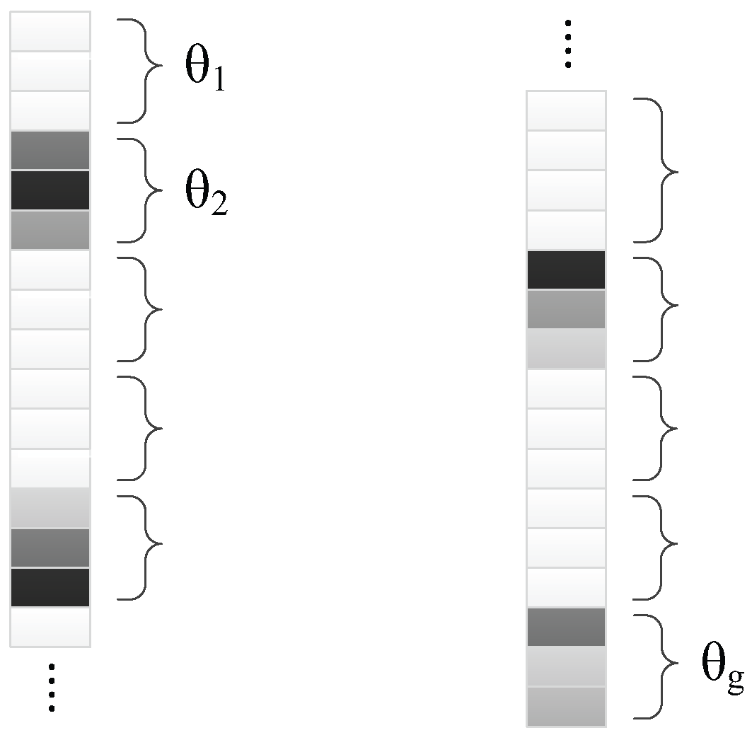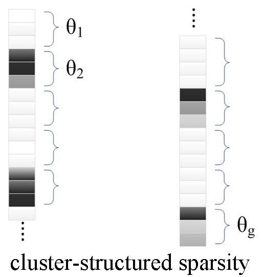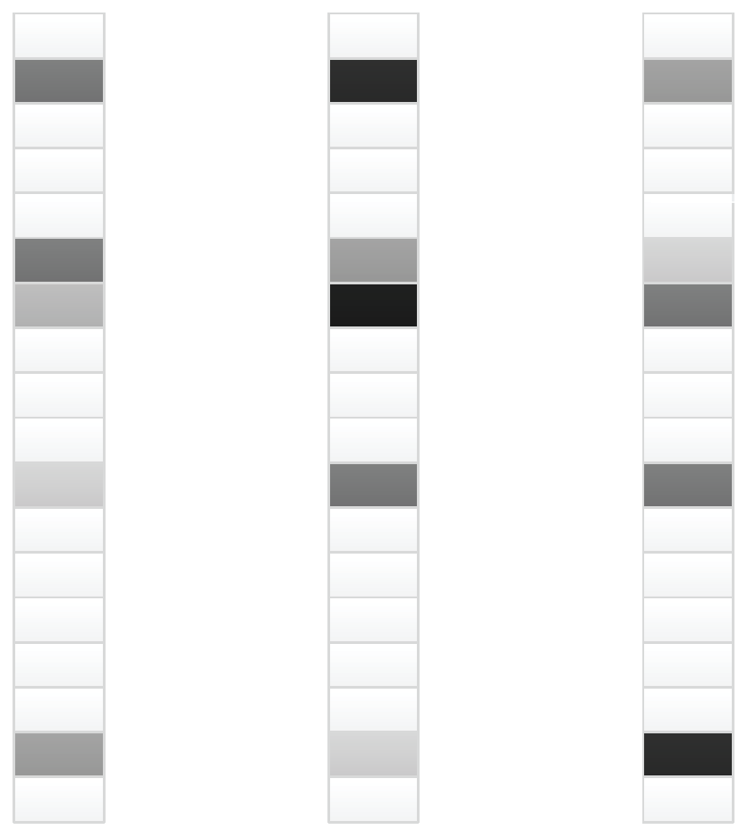For the image patch matrix, we could pick any patch and code it with the coefficient vector θ. Under the assumption of block sparsity, θ could be divided into g continuous groups (see Figure 1):

$$\theta ={\left[{\theta }_1^T,{\theta }_2^T,\cdots ,{\theta }_g^T\right]}^T$$

(3)

The ith group ${\theta }_i$ in θ obeys the parametric joint Gaussian distribution [23]

$$p\left({\theta }_i;{\gamma }_i,B_i\right)\sim N\left(0,{\gamma }_i{B}_i\right)$$

(4)

where ${\gamma }_i$ is non-negative to control the whole sparsity of the ith group, and $B_i$ is a positive semi-definitive matrix to express the correlation level of coefficients in the ith group. ${\gamma }_i$ could be zero and make all the coefficients in the ith group converge to zero, which reflects the structural sparseness at the group level. If θ is considered as the hidden variable, the unknown parameters ${\gamma }_1,\cdots ,{\gamma }_g,B_1,\cdots ,B_g$ could be inferred with expectation maximum (EM). These parameters form the set of hyper-parameters for updating iteratively, as deduced in [17,18].

When the multichannel reconstruction is concerned, coefficients in some different bands, typically the red, green, and blue bands, have similar form of being non-zeros. This happens because these bands have similar local structures. The correlation could be measured with spatial metrics such as structural similarity (SSIM), correlated coefficient (CC), mutual information (MI), etc. The similarity property gives auxiliary prior information for better regularization. In this case, bSBL would also be helpful to a multichannel decomposition. For a patch of three bands (see Figure 2), if we reform the coefficients as a column first, it could be deemed as grouped coefficients with fixed block length equaling three. Then, each ${\gamma }_i$ controls coefficients of all bands in the ith position whether zeros or non-zeros.

3. Spatiotemporal Fusion Framework, Model and Optimization

In this section, the framework of spatiotemporal fusion is firstly introduced, and a new model integrating the semi-coupled dictionary learning and structural sparsity of block sparse Bayesian learning is built to solve this problem. The training method and the prediction method with regard to the proposed model are detailed below.

3.1. Problem Definition

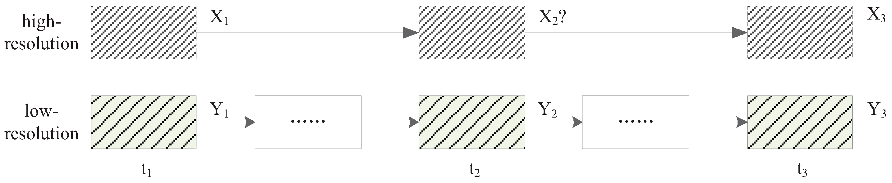
To perform fusion tasks for remote sensing images, the placement of all images should match exactly according to the unique geographic location. As differences exist for projection methods and datums, and geographical calibration errors can hardly be avoided, registration between images should be performed ahead of the fusion for fine geographic calibration. After the registration procedure, shown in Figure 3 the spatiotemporal fusion requires that at least three low-resolution images at times $t_1$, $t_2$ and $t_3$ be provided, as well as high-resolution images of the same locations at times $t_1$ and $t_3$. The high-resolution image at time $t_2$ is, therefore, the target image to be predicted, which is essentially improved in its temporal resolution.

Alternatively, some fusion methods [6,14] used only one known pair $\left\{Y_1,X_1\right\}$ and $Y_2$ to predict $X_2$, which may produce more errors than those using two-pair images. This happens because when we have images from three different times, the differences in image could then be obtained for training. This corresponds to a second-order interpolation that provides a better basis for the predicted images than the first-order interpolation of one-pair images, and thus contributes to higher accuracy than if the original image for reconstruction were used directly.

The differences in images are defined as:

$$\begin{array}{cc}\hfill Y_{21}& =Y_2-Y_1\hfill \\ \hfill X_{21}& =X_2-X_1\hfill \end{array}$$

(5)

$$\begin{array}{cc}\hfill Y_{23}& =Y_2-Y_3\hfill \\ \hfill X_{23}& =X_2-X_3\hfill \end{array}$$

(6)

$$\begin{array}{cc}\hfill Y_{13}& =Y_1-Y_3\hfill \\ \hfill X_{13}& =X_1-X_3\hfill \end{array}$$

(7)

The focus of the spatiotemporal fusion is then to predict the difference image $X_{21}$ from $Y_{21}$ and $X_{23}$ from $Y_{23}$. The integrated outcome of $X_{21}$ and $X_{23}$ is the final prediction image. The difference pair $\left\{Y_{13},X_{13}\right\}$ could then be used to obtain the parameter of prediction. Obviously, $Y_1$, $Y_2$, and $Y_3$ are the up-sampled low-resolution images that have the same spatial resolution to $X_1$ and $X_3$.

The notations used for the whole paper are defined as follows:

X:	the patch matrix extracted from the high-resolution difference image $X_{21}$, $X_{23}$, or $X_{13}$.
Y:	the patch matrix extracted from the geographically matched low-resolution difference image $Y_{21}$, $Y_{23}$, or $Y_{13}$.
DX:	the over-complete Dictionary trained for X.
DY:	the over-complete Dictionary trained for Y.
αX:	the sparse coefficients of X decomposed by $D_X$.
αY:	the sparse coefficients of Y decomposed by $D_Y$.
WX→Y:	the left multiplication matrix mapping from ${\alpha }_X$ to ${\alpha }_Y$.
WY→X:	the left multiplication matrix mapping from ${\alpha }_Y$ to ${\alpha }_X$.
$\left\{{\lambda }_1,{\lambda }_2\right\}$:	adjustable parameters for regularization.

3.2. Incorporating Block Sparseness and Semi-Coupled Dictionary Learning

We propose the following model for spatiotemporal reconstruction by taking the place of the ${\ell }_1$ norm with the constraints of bSBL to represent structural sparseness of coefficients, which is hereafter referred to as bSBL-SCDL—block Sparse Bayesian Learning for Semi-Coupled Dictionary Learning:

$$\begin{array}{cc}\hfill \underset{{\alpha }_X,{\alpha }_Y}{argmin}& {∥X-D_X{\alpha }_X∥}_2^2+{∥Y-D_Y{\alpha }_Y∥}_2^2\hfill \\ & +{\lambda }_1\left({∥{\alpha }_X-W_{Y\to X}{\alpha }_Y∥}_2^2+{∥{\alpha }_Y-W_{X\to Y}{\alpha }_X∥}_2^2\right)\hfill \\ & +{\lambda }_2\left(\mathrm{bSBL}\left({\alpha }_X\right)+\mathrm{bSBL}\left({\alpha }_Y\right)\right),\hfill \end{array}$$

(8)

where

$$\begin{array}{cc}\hfill \mathrm{bSBL}\left({\alpha }_X\right)& ={\sum }_{m}p\left(a_m|X_m;\lambda ,{\gamma }_i,B_i,\forall i\right)\hfill \\ & ={\sum }_{m}N\left({\mu }_{{\alpha }_m},{\mathrm{\Sigma }}_{{\alpha }_m}\right).\hfill \end{array}$$

(9)

The following will give details on training and prediction based on Equation (8). Similar steps could be found in [15]. Before that, the solution to the bSBL constraint is introduced, which will be used in the consequent optimization.

3.3. Optimization to the bSBL Model

For an image patch x that is sparsely represented with an over-complete dictionary D, the bSBL model gives a solution to this problem:

$$\begin{array}{c}\hfill {∥x-D\theta ∥}_2^2+\lambda ·\mathrm{bSBL}\left(\theta \right)\end{array}$$

(10)

where

$$\begin{array}{cc}\hfill \mathrm{bSBL}\left(\theta \right)& =p\left(\theta |x;\lambda ,{\gamma }_i,B_i,\forall i\right)\hfill \\ & =N\left({\mu }_{\theta },{\mathrm{\Sigma }}_{\theta }\right)\hfill \end{array}$$

(11)

For a single-channel image patch x, the solution to θ is listed in Algorithm 1, which corresponds to the Enhanced BSBL Bound Optimization (EBSBL-BO) algorithm with unknown partitions (see [17] for details). To get the Toeplitz form of correlation matrix B, $r=m_1/m_0$, where $m_1$ is the average of the elements among the main sub-diagonal of the matrix B, and $m_0$ is the average of the elements among the main diagonal of the matrix B.

Algorithm 1. bSBL (Block Sparse Bayesian Learning) for single-channel decomposition

1. Initialization:

(1) Set ${\mu }_{\theta }$ to all zeros and γ to all ones.

(2) Set Σ and ${\mathrm{\Sigma }}_0$ to the identity matrix.

(3) Set each $B_i$ to the identity matrix.

2. Repeat until the stop-criterion is reached:

(1) Set the coefficient of the ith block to zero when ${\gamma }_i$ is lower than threshold.

(2) Update the sparse coefficient θ with:

${\theta }^{*}={\mu }_{\theta }={\mathrm{\Sigma }}_0{D}^T{\left(\lambda I+D{\mathrm{\Sigma }}_0{D}^T\right)}^{-1}x$

(3) Update the covariance matrix ${\mathrm{\Sigma }}_{\theta }$ with: ${\mathrm{\Sigma }}_{\theta }={\left({\mathrm{\Sigma }}_0^{-1}+\frac{1}{\lambda }{D}^{T}D\right)}^{-1}$

(4) For each block $i=1,2,\cdots ,g$, get the average correlation matrix B with:

$B=\frac{1}{g}{\sum }_{i=1}^g{B}_i=\frac{1}{g}{\sum }_{i=1}^g\frac{{\mathrm{\Sigma }}_x^i+{\mu }_x^i{\left({\mu }_x^i\right)}^T}{{\gamma }_i}$

(5) For each block $i=1,2,\cdots ,g$, constrain $B_i$ to an approximal Toeplitz form:

$B_i=B=\mathrm{Toeplitz}\left(\left[1,r,\cdots ,r^{d-1}\right]\right)$

(6) For each block $i=1,2,\cdots ,g$, update the general block sparsity ${\gamma }_i$ with:

${\gamma }_i=\sqrt{\frac{x_i^T{B}_i^{-1}{x}_i}{\mathrm{Tr}\left({\left(D^i\right)}^T{\left({\mathrm{\Sigma }}_y^{*}\right)}^{-1}{D}^i{B}_i\right)}}$, ${\mathrm{\Sigma }}_y^{*}=\lambda I+D^i{\mathrm{\Sigma }}_0{\left(D^i\right)}^T$

(7) Update the unconstrained weight λ with:

$\lambda =\frac{{∥x-D{\mu }_{\theta }∥}_2^2+\mathrm{Tr}\left({\mathrm{\Sigma }}_{\theta }{D}^{T}D\right)}{M}$

(8) Update ${\mathrm{\Sigma }}_0$ with:

${\mathrm{\Sigma }}_0=diag\left({\gamma }_1,\cdots ,{\gamma }_M\right)\otimes B$

For a multichannel image patch x, the solution to θ could be found with Algorithm 2, which is modified by us from the bSBL Bound Optimization (BSBL-BO) algorithm with known partitions (see [17] for details). Note that θ and y are 2-D matrix in which different bands are aligned column by column.

Algorithm 2. bSBL (Block Sparse Bayesian Learning) for multichannel decomposition

1. Initialization:

(1) Set ${\mu }_{\theta }$ to all zeros and γ to all ones.

(2) Set Σ and ${\mathrm{\Sigma }}_0$ to the identity matrix.

2. Repeat until the stop-criterion is reached:

(1) Set the coefficient of the ith position to zero when ${\gamma }_i$ is lower than threshold.

(2) Update the sparse coefficient θ with:

${\theta }^{*}={\mu }_{\theta }={\mathrm{\Sigma }}_0{D}^T{\left(\lambda I+D{\mathrm{\Sigma }}_0{D}^T\right)}^{-1}x$

(3) Update the covariance matrix ${\mathrm{\Sigma }}_{\theta }$ with:

${\mathrm{\Sigma }}_{\theta }={\left({\mathrm{\Sigma }}_0^{-1}+\frac{1}{\lambda }{D}^{T}D\right)}^{-1}$

(4) For each block $i=1,2,\cdots ,g$, update the general block sparsity ${\gamma }_i$ with:

${\gamma }_i=\sqrt{\frac{{\gamma }_i{\theta }_i^T{\theta }_i}{\mathrm{Tr}\left({\left(D^i\right)}^T{D}^i\right)}}$

(5) Update the unconstrained weight λ with:

$\lambda =\frac{{∥x-D{\mu }_{\theta }∥}_2^2+\mathrm{Tr}\left({\mathrm{\Sigma }}_{\theta }{D}^{T}D\right)}{M}$

(6) Update ${\mathrm{\Sigma }}_0$ with:

${\mathrm{\Sigma }}_0=diag\left(\left\{{\gamma }_i\right\}\right)$

3.4. Training

The following steps are used to train dictionary pairs and coefficient mapping matrix of high- and low-resolution patches. Preprocessing and clustering are performed before dictionaries are coupled.

(1)

Preprocessing images of time $t_1$ and $t_3$

The difference images $X_{31}$ and $Y_{31}$ are calculated, and divided into patches. Each patch removes the mean value and is normalized to 1 under the ${\ell }_2$ norm.

(2)

Clustering

A clustering method (e.g., the k-means algorithm) is employed for the patch $X_{31}$ set to classify the patches into different categories according to the distance to the clustered centers.

The following flows are processed independently for each class. To do this, a bank of high-resolution patches of the same class is extracted to form the new X, and their counterpart low-resolution patches form the new Y.

(1)

Initialization

The sparse coefficients are initially assumed to be the same, i.e., ${\alpha }_X={\alpha }_Y={\alpha }_0$. A dictionary learning method (e.g., online dictionary learning or K-SVD) can then be used to solve the following:

$$\underset{{\alpha }_0}{argmin}{∥X-D_X{\alpha }_0∥}_2^2+{∥Y-D_Y{\alpha }_0∥}_2^2+{\lambda }_1{∥{\alpha }_0∥}_1$$

(12)

This gives the initial dictionary pair $D_X$ and $D_Y$.

Then, the bSBL constraint is used to obtain a new ${\alpha }_0$ by solving the following:

$$\begin{array}{cc}& \underset{{\alpha }_0}{argmin}{∥X-D_X{\alpha }_0∥}_2^2+{∥Y-D_Y{\alpha }_0∥}_2^2+{\lambda }_2·\mathrm{bSBL}\left({\alpha }_0\right)\hfill \\ \hfill =& \underset{{\alpha }_0}{argmin}{∥\left[\begin{array}{c}X\\ Y\end{array}\right]-\left[\begin{array}{c}{D}_X\\ D_Y\end{array}\right]{\alpha }_0∥}_2^2+{\lambda }_2·\mathrm{bSBL}\left({\alpha }_0\right)\hfill \end{array}$$

(13)

$W_{X\to Y}$ and $W_{Y\to X}$ are initialized to be the identity matrix.

(2)

Updating dictionaries and mapping matrix

${\alpha }_Y$ is updated with

$$\begin{array}{cc}\hfill {\alpha }_Y=\underset{{\alpha }_Y}{argmin}& {∥Y-D_Y{\alpha }_Y∥}_2^2+{\lambda }_1{∥{\alpha }_X-W_{Y\to X}{\alpha }_Y∥}_2^2\hfill \\ & +{\lambda }_2·\mathrm{bSBL}\left({\alpha }_Y\right)\hfill \\ \hfill =\underset{{\alpha }_Y}{argmin}& {∥\left[\begin{array}{c}Y\\ {\lambda }_1{\alpha }_X\end{array}\right]-\left[\begin{array}{c}{D}_Y\\ {\lambda }_1{W}_{Y\to X}\end{array}\right]{\alpha }_Y∥}_2^2+{\lambda }_2·\mathrm{bSBL}\left({\alpha }_Y\right)\hfill \end{array}$$

(14)

${\alpha }_X$ is updated with

$$\begin{array}{cc}\hfill {\alpha }_X=\underset{{\alpha }_X}{argmin}& {∥X-D_X{\alpha }_X∥}_2^2+{\lambda }_1{∥{\alpha }_Y-W_{X\to Y}{\alpha }_X∥}_2^2\hfill \\ & +{\lambda }_2·\mathrm{bSBL}\left({\alpha }_X\right)\hfill \\ \hfill =\underset{{\alpha }_X}{argmin}& {∥\left[\begin{array}{c}X\\ {\lambda }_1{\alpha }_Y\end{array}\right]-\left[\begin{array}{c}{D}_X\\ {\lambda }_1{W}_{X\to Y}\end{array}\right]{\alpha }_X∥}_2^2+{\lambda }_2·\mathrm{bSBL}\left({\alpha }_X\right)\hfill \end{array}$$

(15)

Dictionaries $D_Y$ and $D_X$ are updated with dictionary learning methods.

$W_{Y\to X}$ and $W_{X\to Y}$ could be directly obtained by solving the least square equations

$$\begin{array}{c}{W}_{Y\to X}=\underset{W_{Y\to X}}{argmin}{∥{\alpha }_X-W_{Y\to X}{\alpha }_Y∥}_2^2\hfill \\ W_{X\to Y}=\underset{W_{X\to Y}}{argmin}{∥{\alpha }_Y-W_{X\to Y}{\alpha }_X∥}_2^2\hfill \end{array}$$

(16)

The iteration stops when it reaches the maximal number or the total cost does not decrease any more.

This process is repeated until all classes have trained the dictionary pair $\left\{D_X,D_Y\right\}$ and the mapping relations $\left\{W_{Y\to X},W_{X\to Y}\right\}$.

3.5. Prediction

To perform spatiotemporal fusion, the patch matrix from the low-resolution difference image $Y_{21}$ and $Y_{23}$ are presented, which are used to predict the reconstruction image independently. For simplicity, the patch matrix of $Y_{21}$ or $Y_{23}$ is abbreviated as Y, while the predicted images is X.

(1)

Classification

All patches are categorized into different classes according to the distance to the clustering centers that were produced during the training stage.

(2)

Initialization

A class of patches is chosen to form the new Y. The dictionary pair $\left\{D_X,D_Y\right\}$ and the mapping correlation $\left\{W_{Y\to X},W_{X\to Y}\right\}$ linking to this class are picked from the trained parameters.

The initial ${\alpha }_Y$, ${\alpha }_X$, and X are obtained by solving the following:

$$\begin{array}{cc}\hfill {\alpha }_Y& =\underset{{\alpha }_Y}{argmin}{∥Y-D_Y{\alpha }_Y∥}_2^2+{\lambda }_2·\mathrm{bSBL}\left({\alpha }_Y\right)\hfill \\ \hfill {\alpha }_X& =W_{Y\to X}*{\alpha }_Y\hfill \\ \hfill X& =D_X*{\alpha }_X\hfill \end{array}$$

(17)

(3)

Updating the predicted image iteratively

Update ${\alpha }_Y$:

$$\begin{array}{cc}\hfill {\alpha }_Y=\underset{{\alpha }_Y}{argmin}& {∥Y-D_Y{\alpha }_Y∥}_2^2+{\lambda }_1{∥{\alpha }_X-W_{Y\to X}{\alpha }_Y∥}_2^2\hfill \\ & +{\lambda }_2·\mathrm{bSBL}\left({\alpha }_Y\right)\hfill \\ \hfill =\underset{{\alpha }_Y}{argmin}& {∥\left[\begin{array}{c}Y\\ {\lambda }_1{\alpha }_X\end{array}\right]-\left[\begin{array}{c}{D}_Y\\ {\lambda }_1{W}_{Y\to X}\end{array}\right]{\alpha }_Y∥}_2^2+{\lambda }_2·\mathrm{bSBL}\left({\alpha }_Y\right)\hfill \end{array}$$

(18)

Update ${\alpha }_X$:

$$\begin{array}{cc}\hfill {\alpha }_X=\underset{{\alpha }_X}{argmin}& {∥X-D_X{\alpha }_X∥}_2^2+{\lambda }_1{∥{\alpha }_Y-W_{X\to Y}{\alpha }_X∥}_2^2\hfill \\ & +{\lambda }_2·\mathrm{bSBL}\left({\alpha }_X\right)\hfill \\ \hfill =\underset{{\alpha }_X}{argmin}& {∥\left[\begin{array}{c}X\\ {\lambda }_1{\alpha }_Y\end{array}\right]-\left[\begin{array}{c}{D}_X\\ {\lambda }_1{W}_{X\to Y}\end{array}\right]{\alpha }_X∥}_2^2+{\lambda }_2·\mathrm{bSBL}\left({\alpha }_X\right)\hfill \end{array}$$

(19)

Update X:

$$X=D_X*{\alpha }_X$$

(20)

4. Experiments and Validation

Performance of the proposed fusion method is evaluated in this section, which is compared with four state-of-the-art methods that were proposed recently to show the validation. The comparison demonstrates the digital differences and visual differences when these methods are used to fuse images of MODIS and Landsat-7.

4.1. Experimental Scheme

Five spatiotemporal fusion methods are used for fusion, including STARFM [6], class-RSpatialU [11], EBSCDL [15], and the bSBL-SCDL method proposed in this paper. An additional algorithm is the multichannel version of bSBL-SCDL, which we called msSBL-SCDL. The parameters of bSBL-SCDL are set as follows: size of each image patch is 5 × 5, γ is 0.01, ${\lambda }_1$ is 0.01, dictionary size is 128, classified number is 32, and the block length of bSBL is 3 with unknown partitions. These parameters are also used by SCDL and EBSCDL. ${\lambda }_2$ of EBSCDL is 0.1. Parameters of msSBL-SCDL are exactly the same as bSBL-SCDL.

The red, green, and near-infrared (NIR) bands of the reflection products from Landsat-7 ETM+ and MODIS multispectral (MS) sensors are selected as the source images for fusion. These images have been used in [6,15]. Here, we divided them into multiple 300 × 300-size images for comparison. The Landsat-7 ETM+ images have a revisiting period of 16 days with 30 m of the ground resolution, while the MODIS MS images could be captured daily with 500 m of the ground resolution. The data used in this paper were captured on 24 May, 11 July, and 12 August of 2001, respectively. The Landsat-7 data on 11 July 2001 was set as the data to be reconstructed, which would be verified with the real data to determine the performance of the comparison algorithms. Before the fusion was performed, each low-resolution image was scaled to the same resolution as that of high-resolution images.

High structural correlation was the initial motivation that msSBL-SCDL works. We could find, however, that high correlation exists only between the red band and the green band. For example, we tested the structural similarity between bands of the ground image to be predicted with the metric of SSIM, which are 0.7993 for red-green, 0.0654 for red-NIR, and 0.0952 for green-NIR. The evaluated numbers of correlation coefficients are 0.9570 for red-green, 0.4200 for red-NIR, and 0.5169 for green-NIR. Therefore, we used msSBL-SCDL only for the red band and the green band as a whole.

4.2. Comparative Summary: Prediction Performance

The root mean square error (RMSE) of fused images with respect to varied algorithms were measured for performance validation by comparing the predicted images to the real images—see

Table 1. Reflectance root mean square error (RMSE) of the Red Band.

Image Number	1	2	3
mean	0.0345	0.0367	0.0355
stdvar	0.0141	0.0124	0.0108
STARFM	0.0105	0.0058	0.0067
class-RSpatialU	0.0106	0.0061	0.0056
SCDL	0.0108	0.0060	0.0058
EBSCDL	0.0108	0.0060	0.0058
bSBL-SCDL	0.0102	0.0055	0.0059
msSBL-SCDL	0.0104	0.0059	0.0062

,

Table 2. Reflectance RMSE of the Green Band.

Image Number	1	2	3
mean	0.0476	0.0511	0.0487
stdvar	0.0121	0.0079	0.0084
STARFM	0.0098	0.0042	0.0044
class-RSpatialU	0.0110	0.0065	0.0065
SCDL	0.0102	0.0039	0.0040
EBSCDL	0.0102	0.0039	0.0040
bSBL-SCDL	0.0095	0.0037	0.0038
msSBL-SCDL	0.0095	0.0037	0.0038

and

Table 3. Reflectance RMSE of the NIR Band.

Image Number	1	2	3
mean	0.2113	0.2249	0.2320
stdvar	0.0383	0.0413	0.0413
STARFM	0.0200	0.0164	0.0179
class-RSpatialU	0.0263	0.0283	0.0343
SCDL	0.0192	0.0153	0.0164
EBSCDL	0.0191	0.0154	0.0164
bSBL-SCDL	0.0190	0.0150	0.0173

. The peak signal-to-noise ratio (PSNR) was not evaluated because reflectance ranges from 0 to 1. As RMSE is not the most suitable metric for remote sensing applications when spectral loss is involved , some popular metrics are also used in

Table 4. Spectral evaluation of NIR/Red/Green bands: image 1.

	SAM	RASE	ERGAS	Q4
STARFM	0.0314	0.1452	0.0546	0.7933
class-RSpatialU	0.0339	0.1793	0.0582	0.7394
SCDL	0.0307	0.1431	0.0563	0.8086
EBSCDL	0.0307	0.1429	0.0563	0.8094
bSBL-SCDL	0.0296	0.1395	0.0534	0.8105

and

Table 5. Spectral evaluation of NIR/Red/Green bands: image 3.

	SAM	RASE	ERGAS	Q4
STARFM	0.0311	0.1057	0.0291	0.8903
class-RSpatialU	0.0371	0.1939	0.0366	0.8161
SCDL	0.0300	0.0977	0.0284	0.9107
EBSCDL	0.0300	0.0976	0.0284	0.9110
bSBL-SCDL	0.0308	0.1023	0.0285	0.8970

, including spectral angle mapper (SAM), relative average spectral error (RASE) [24], Erreur Relative Globale Adimensionnelle de Synthese (ERGAS) [25], and Q4 [26]. Note that the ideal result is 0 for SAM, RASE, and ERGAS, while it is 1 for Q4. msSBL-SCDL was only evaluated in Table 1 and Table 2 due to the correlation limit between bands.

The digital evaluation of Table 1, Table 2 and Table 3 shows that all these methods could reconstruct the “unknown” high-resolution image for the given time effectively. STARFM, SCDL, EBSCDL, bSBL-SCDL, and msSBL-SCDL perform steadily in producing similar digital errors. The differences between SCDL and EBSCDL are hardly distinguished. The bSBL-SCDL and msSBL-SCDL methods that we proposed in this paper could slightly outweigh other methods in most cases. Table 2 shows that bSBL-SCDL and msSBL-SCDL produced very similar results for the green band, but Table 1 shows that bSBL-SCDL could outperform msSBL-SCDL for the red band.

The spectral evaluation of Table 4 and Table 5 illustrates that SCDL, EBSCDL and bSBL-SCDL could maintain a slightly higher spectral fidelity than methods of STARFM and class-RSpatialU, which offers substantial benefits for remote sensing applications. Our bSBL-SCDL method produces the least spectral distortion for image 1 and just a bit more for image 3.

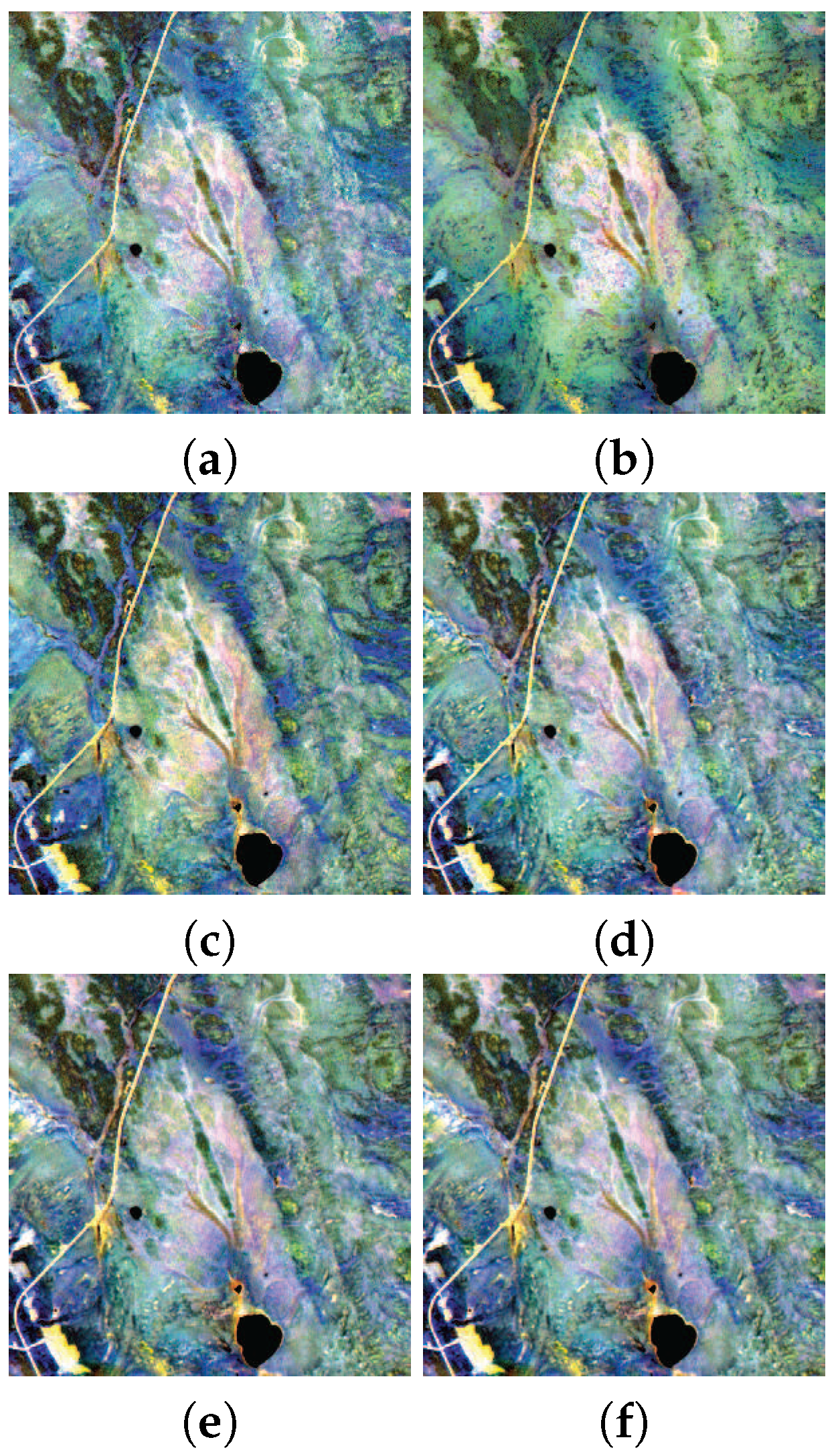
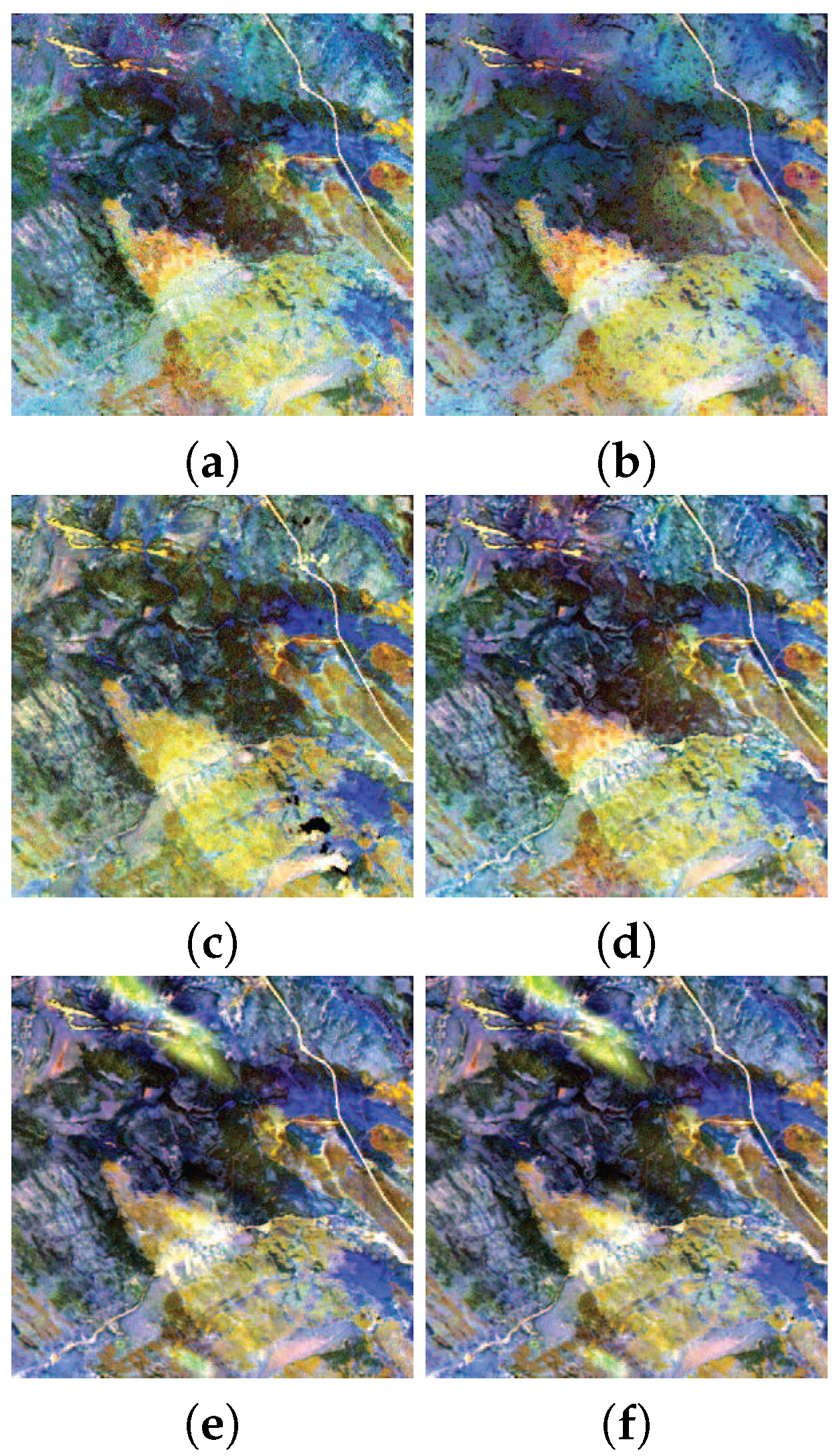
Figure 4 and Figure 5 are displayed with the tool of ENVI 2% enhancement. As the histogram distributions of reconstructed images are not exactly the same, the spectral evaluation is more trustworthy than displayed colors. However, the degree of spatial enhancement is distinguishable, which shows that STARFM and class-RSpatialU reconstruct textural details well, while SCDL, EBSCDL, and bSBL-SCDL reconstruct more structural details.

5. Discussion

We noticed that, in the comparison of the third reconstruction of the NIR band, bSBL-SCDL is inferior to SCDL and EBSCDL. To disclose the reason, the produced images were compared block by block. Then, it is confirmed that the differences exist mainly in some smoothing areas. Specifically, our method produced even more details than expected in these areas. This is quite possibly due to the insufficient coefficients sparsity for the plain terrestrial content. However, in the areas of rich edges and contours, bSBL-SCDL could perform better steadily. This shows that the proposed method could be further improved either by treating the smoothing areas separately or by integrating other fusion methods that have slight advantages for smoothing content. Additionally, msSBL-SCDL could be expected to obtain even better results when more correlated bands, for instance the red, green, and blue bands, are involved.

The images in Figure 4 and Figure 5 could explain the characteristics of two classes of spatiotemporal fusion methods. Combining methods (STARFM and class-RSpatialU) in a linear fashion has advantages for the seasonally changing areas, typically forests and water. By observing the structures within images, it is confirmed that sparse representation methods, including SCDL, EBSCDL, and bSBL-SCDL, could produce even richer edges and contours. Therefore, the latter method could perform better for applications of urban environments. The former class is relatively simple and fast, which is suitable for statistical applications of vegetation and crops.

The relative radiometric error (RAE) could be otained with RAE = RMSE/mean. Then, the best RAEs of all images are calculated: 29.61%, 15.02%, 16.49%, 19.99%, 7.31%, 7.85%, 9.01%, 6.68%, and 7.47%. It is evident that the red and green band of image 1 fall out of the acceptable range of 15% maximum errors. This could be explained with the detail level of “stdvar/mean”. It then becomes clear that the challenging issue still exists in predicting images of rich details.

The main obstacle of the bSBL-SCDL algorithm that we proposed in this paper is the processing speed. Generally, it requires a long time to produce an optimization solution. Two possible accelerations are therefore considered in the future work: coding with OPENMP/MPI/GPU support for parallel running, or improving the bSBL optimization method theoretically.

6. Conclusions

In this paper, we proposed a fusion method to integrate remote sensing images of different spatial and temporal resolutions to construct new images of high spatial and temporal resolutions. The new method follows the concept of coupling dictionaries and coefficients of images of the same content from different sensors, but the critical sparse term of coded coefficients is replaced with the block sparseness constraint to find even more accurate coefficients. The new regularization method is significant for the spatiotemporal fusion task because the inaccurate sparse representation in the training stage would be amplified when it is used for prediction.

We named the proposed method as bSBL-SCDL for single-channel prediction and msSBL-SCDL for multichannel prediction. bSBL-SCDL could improve the prediction accuracy because it employs the structural sparseness property of coefficient that makes better approximation to the ${\ell }_0$ norm than the ${\ell }_1$-norm solutions from LASSO, OMP, and so on. msSBL-SCDL, on the other hand, employs the property that coefficients of highly correlated bands should have similar sparseness distribution. To validate this, we compared them with some state-of-the-art fusion methods including STARFM, class-RSpatialU, SCDL, EBSCDL using the red, green, and NIR bands of Landsat-7 and MODIS. The experiment shows that, in most cases, the proposed bSBL-SCDL method obtained the best reconstruction results under the metric of root mean square errors. Quantitatively for the red and green bands, bSBL-SCDL is around 5% better than SCDL and EBSCDL, and 3%–20% better than STARFM. For the NIR band, bSBL-SCDL shows a similar performance to SCDL and EBSCDL, but is obviously better than STARFM. This proves that its reconstruction is generally closer to the real images than other latest methods. The proposed msSBL-SCDL could also slightly improve the reconstruction performance for the red and green band.

References

- Rodger, J.A. Toward reducing failure risk in an integrated vehicle health maintenance system: A fuzzy multi-sensor data fusion Kalman filter approach for IVHMS. Expert Syst. Appl. 2012, 39, 9821–9836. [Google Scholar] [CrossRef]
- He, Z.; Wu, C.; Liu, G.; Zheng, Z.; Tian, Y. Decomposition tree: A spatio-temporal indexing method for movement big data. Clust. Comput. 2015, 18, 1481–1492. [Google Scholar] [CrossRef]
- Wang, Y.; Liu, Z.; Liao, H.; Li, C. Improving the performance of GIS polygon overlay computation with MapReduce for spatial big data processing. Clust. Comput. 2015, 18, 507–516. [Google Scholar] [CrossRef]
- Chen, Y.; Li, F.; Fan, J. Mining association rules in big data with NGEP. Clust. Comput. 2015, 18, 577–585. [Google Scholar] [CrossRef]
- Deng, Z.; Hu, Y.; Zhu, M.; Huang, X.; Du, B. A scalable and fast OPTICS for clustering trajectory big data. Clust. Comput. 2015, 18, 549–562. [Google Scholar] [CrossRef]
- Gao, F.; Masek, J.; Schwaller, M.; Hall, F. On the blending of the Landsat and MODIS surface reflectance: Predicting daily Landsat surface reflectance. IEEE Trans. Geosci. Remote Sens. 2006, 44, 2207–2218. [Google Scholar]
- Zhu, X.; Chen, J.; Gao, F.; Chen, X.; Masek, J.G. An enhanced spatial and temporal adaptive reflectance fusion model for complex heterogeneous regions. Remote Sens. Environ. 2010, 114, 2610–2623. [Google Scholar] [CrossRef]
- Hilker, T.; Wulder, M.A.; Coops, N.C.; Linke, J.; McDermid, G.; Masek, J.G.; Gao, F.; White, J.C. A new data fusion model for high spatial- and temporal-resolution mapping of forest disturbance based on Landsat and MODIS. Remote Sens. Environ. 2009, 113, 1613–1627. [Google Scholar] [CrossRef]
- Wu, M.; Niu, Z.; Wang, C.; Wu, C.; Wang, L. Use of MODIS and Landsat time series data to generate high-resolution temporal synthetic Landsat data using a spatial and temporal reflectance fusion model. J. Appl. Remote Sens. 2012, 6, 339–355. [Google Scholar]
- Huang, B.; Wang, J.; Song, H.; Fu, D.; Wong, K. Generating high spatiotemporal resolution land surface temperature for urban heat island monitoring. IEEE Geosci. Remote Sens. Lett. 2013, 10, 1011–1015. [Google Scholar] [CrossRef]
- Xu, Y.; Huang, B.; Xu, Y.; Cao, K.; Guo, C.; Meng, D. Spatial and temporal image fusion via regularized spatial unmixing. IEEE Geosci. Remote Sens. Lett. 2015, 12, 1362–1366. [Google Scholar]
- Li, X.; Wang, L. On the study of fusion techniques for bad geological remote sensing image. J. Ambient Intell. Humaniz. Comput. 2015, 6, 141–149. [Google Scholar] [CrossRef]
- Huang, B.; Song, H. Spatiotemporal reflectance fusion via sparse representation. IEEE Trans. Geosci. Remote Sens. 2012, 50, 3707–3716. [Google Scholar] [CrossRef]
- Song, H.; Huang, B. Spatiotemporal satellite image fusion through one-pair image learning. IEEE Trans. Geosci. Remote Sens. 2013, 51, 1883–1896. [Google Scholar] [CrossRef]
- Wu, B.; Huang, B.; Zhang, L. An error-bound-regularized sparse coding for spatiotemporal reflectance fusion. IEEE Trans. Geosci. Remote Sens. 2015, 53, 6791–6803. [Google Scholar] [CrossRef]
- Baraniuk, R.G.; Cevher, V.; Duarte, M.F.; Hegde, C. Model-based compressive sensing. IEEE Trans. Inf. Theory 2010, 56, 1982–2001. [Google Scholar] [CrossRef]
- Zhang, Z.; Rao, B.D. Extension of SBL algorithms for the recovery of block sparse signals with intra-block correlation. IEEE Trans. Signal Process. 2013, 61, 2009–2015. [Google Scholar] [CrossRef]
- Zhang, Z.; Rao, B.D. Sparse signal recovery with temporally correlated source vectors using sparse bayesian learning. IEEE J. Sel. Top. Signal Process. 2011, 5, 912–926. [Google Scholar] [CrossRef]
- Majumdar, A.; Ward, R.K. Compressed sensing of color images. Signal Process. 2010, 90, 3122–3127. [Google Scholar] [CrossRef]
- Gao, F.; Hilker, T.; Zhu, X.; Anderson, M.; Masek, J.; Wang, P.; Yang, Y. Fusing landsat and MODIS data for vegetation monitoring. IEEE Geosci. Remote Sens. Mag. 2015, 3, 47–60. [Google Scholar] [CrossRef]
- Wang, S.; Zhang, L.; Liang, Y.; Pan, Q. Semi-coupled dictionary learning with applications to image super-resolution and photo-sketch synthesis. In Proceedings of the 2012 IEEE Conference on Computer Vision and Pattern Recognition (CVPR), Providence, RI, USA, 16–21 June 2012; pp. 2216–2223.
- Dong, C.; Loy, C.C.; He, K.; Tang, X. Image super-resolution using deep convolutional networks. IEEE Trans. Pattern Anal. Mach. Intell. 2016, 38, 295–307. [Google Scholar] [CrossRef] [PubMed]
- Wipf, D.P.; Rao, B.D. Sparse Bayesian learning for basis selection. IEEE Trans. Signal Process. 2004, 52, 2153–2164. [Google Scholar] [CrossRef]
- Zhang, Y. Methods for image fusion quality assessment—A review, comparison and analysis. Int. Arch. Photogramm. Remote Sens. Spat. Inf. Sci. 2008, 37, 1101–1109. [Google Scholar]
- Ranchin, T.; Wald, L. Fusion of high spatial and spectral resolution images: The ARSIS concept and its implementation. Photogramm. Eng. Remote Sens. 2000, 66, 49–61. [Google Scholar]
- Alparone, L.; Baronti, S.; Garzelli, A.; Nencini, F. A global quality measurement of pan-sharpened multispectral imagery. IEEE Geosci. Remote Sens. Lett. 2004, 1, 313–317. [Google Scholar] [CrossRef]
© 2016 by the authors; licensee MDPI, Basel, Switzerland. This article is an open access article distributed under the terms and conditions of the Creative Commons Attribution (CC-BY) license (http://creativecommons.org/licenses/by/4.0/).