Sea Surface Temperature Retrieval from MODIS Radiances Using Truncated Total Least Squares with Multiple Channels and Parameters

Abstract

Global sea-surface temperatures (SST) from MODIS measured brightness temperatures generated using the regression methods, have been available to users for more than a decade, and are used extensively for a wide range of atmospheric and oceanic studies. However, as evidenced by a number of studies, there are indications that the retrieval quality and cloud detection are somewhat sub-optimal. To improve the performance of both of these aspects, we endorse a new physical deterministic algorithm, based on truncated total least squares (TTLS), using multiple channels and parameters, in conjunction with a hybrid cloud detection scheme using a radiative transfer model atop a functional spectral difference method. The TTLS method is a new addition that improves the information content of the retrieval compared to our previous work using modified total least squares (MTLS), which is feasible because more measurements are available, allowing a larger retrieval vector. A systematic study is conducted to ascertain the appropriate channel selection for SST retrieval from the 16 thermal infrared channels available from the MODIS instrument. Additionally, since atmospheric aerosol is a well-known source of degraded quality of SST retrieval, we include aerosol profiles from numerical weather prediction in the forward simulation and include the total column density of all aerosols in the retrieval vector of our deterministic inverse method. We used a slightly modified version of our earlier reported cloud detection algorithm, namely CEM (cloud and error mask), for this study. Time series analysis of more than a million match-ups shows that our new algorithm (TTLS+CEM) can reduce RMSE by ~50% while increasing data coverage by ~50% compared to the operationally available MODIS SST.

1. Introduction

One of the key variables of the climate system is sea-surface temperature (SST). This is widely used to define the physical environment, and impacts the variability of marine ecosystems [1,2], and is designated an Essential Climate Variable. Water masses defined by marine thermal fronts are often denoted by using SST gradient fields as a proxy, thus identifying regions of optimal conditions for growth of marine phytoplankton (nutrients, light, mixing, and upwelling) and, in many cases, enhanced trophic levels of productivity [3,4,5,6,7]. The spatial and temporal patterns in SST fields are a key characteristic of fisheries ecosystems, having implications for sustainable management [8,9]. In terms of meteorology and climate, SST has a major impact on gas exchange between ocean and the atmosphere, as well as on energy exchanges, such as long-wave radiation, and latent and sensible heat flux (e.g., [1,10,11]). It is also a fundamental quantity in numerical ocean models, climate, and marine weather [2,10]. The long-term record of SST began with bucket temperatures obtained from sailing vessels; more modern SST observations are made by moored and drifting buoys, ship intake, CTD (conductivity, temperature and depth profiler) casts, in situ radiometers carried on research vessels, and, increasingly, satellites [12]. The advantages of satellite-derived SST are vast coverage at high resolution compared to any other form of collected SST data from relatively few sources. Among the satellite derived SST products, MODIS (MODerate resolution Imaging Spectroradiometers) SSTs has an impressive long-term data record (~15 years) from a single sensor, and is used for a wide variety of oceanographic and atmospheric applications, e.g., ocean circulation modeling, numerical weather prediction, boundary currents, air–sea interactions, upwelling regions, studies of planetary boundary layer divergence, ocean biology, including algae blooms, and coral reefs (e.g., [13,14,15,16,17,18,19,20]). The performance of these studies always depends on the accuracy of SST retrieval and data coverage of MODIS measurement.

Great potential is on offer with the MODIS instrument, which makes information-rich multiband measurements with a high signal-to-noise ratio, thus, the prospects are good for improving both the quality and coverage of SST data. However, much of this potential remains unrealized, primarily because of the inverse methods that have been used, thus far, in the operationally derived products, which still employ regression of only two or three channels, (e.g., [2,21,22,23]). In previous decades, when computational resources were limited, such approaches were justifiable in the interest of obtaining a reasonable processing time. However, such approaches are evidently inadequate when trying to characterize global geophysical conditions (atmospheric and oceanic states) for SST retrievals using only a small number of regression coefficients. In addition, assigning error associated to individual retrievals, which is highly desirable, is difficult for regression-based SST retrievals. In addition, aerosol is one of the main hurdles to reduce retrieved SST errors from MODIS measurements (e.g., [12,24]), and it is very difficult to mitigate this problem using the currently-implemented operational retrieval method. The above-mentioned reasons, together with the availability of improved computational capability and the wealth of channels in MODIS instruments, urge the development of forward, model-based, multi-channels SST retrievals, both feasible and desirable, and are considered in this paper.

Cloud detection is a key aspect of any parameter estimation using satellite IR measurements. The operational MODIS cloud detection scheme primarily makes use of observed spectral differences. Accurate cloud-masks using such differences, alone, is extremely challenging, thus, spatial coherence tests are also employed. However, cloud contamination remains one of the significant error contributions in the operational MODIS SST product, as reported in a number of studies (e.g., [2,12,22]). To improve cloud detection, we hereby introduce various radiative transfer (RT) based classification tests, on top of a somewhat relaxed functional spectral differences approach, including relaxed spatial coherence tests.

2. Data and Methods

We use the same data and collocation procedure as reported in our earlier publication [25]. We have collocated GHRSST MODIS-A SST, buoy SST, GFS, MODIS-A L1b BT and MODIS-A geolocation data, which provide us with point matches. The match-up window of this monthly matchup database (MMDB) was set to ±30 min for buoys coincident within satellite pixels. After collocation, this MMDB provides BTs from the MODIS-A, and National Centers for Environmental Prediction (NCEP) surface and upper-air forecast fields. Quality controlled data from NOAA iQuam [26] are used as the in situ source, mainly buoys (SST_b). Drifters, tropical moorings, and coastal moorings are used in this study. The coastal moorings are often considered problematic, but actually furnish us with many of the more extreme departures from first-guess SST due to being in high-gradient regions, and are, thus, invaluable tests of physical retrieval methods. We refer to the surface temperature from NCEP as the initial guess (IG) SST (SST_g). We use the CRTM for forward modeling that, in the future, can also be used in an operational environment to minimize computational cost. Simulated Brightness temperatures (BTs) were calculated employing the CRTM v2.1 with NCEP data as input to provide the necessary inputs for physically-based retrieval methods. NOAA environmental modeling system GFS Aerosol Component (NGAC) is a global in-line aerosol forecast system and 15 different species aerosol profiles from NGAC are used. We intend to develop this algorithm for near-real-time operational compatibility, thus, we chosen forecast data instead of a reanalysis of data. We have also used the CRTM-derived partial derivatives (Jacobians) of the channel BTs, with respect to surface temperature (δy_λ/δs), and logarithm of total column water vapor (TCWV) (δy_λ/δw), where w = ln(TCWV). We have restricted this study to night-only retrievals to avert the traditional concerns, and, at the time of writing, the shortwave component of the CRTM does not adequately cover the 4-μm region. A constant offset of −0.17 K to account for the skin bulk SST differences of buoy was used as a first-order approximation for nighttime data [27].

In our previous work [28], we have introduced a physical deterministic inverse method, modified total least squares (MTLS), which was shown to outperform other prevalent methods for SST retrieval from GOES-13 imager measurements. However, as we have discussed in an earlier publication, TLS yields good retrievals when the condition number of the Jacobian is low for a given problem. However, as the RT problem is inherently ill-conditioned and the error amplification from the measurement space to the state space is proportional to the condition number of Jacobian [29]. Thus, the regularized TLS (RTLS) (e.g., [30]) or truncated TLS (TTLS) are most commonly used. We discussed that such methods (e.g., TTLS) could not be implemented because of the limited number of spectral channels in GOES-13 data (only 3 usable SST retrieval channels). Using the MODIS instrument, which has an increased spectral capability, opens up the opportunity to test TTLS methods. We have already reported [25,28,31,32] that the physical deterministic MTLS methods for SST retrieval from MODIS and GOES-13 are far better than the stochastic optimal estimation method (OEM), since there are inherent ambiguities; OEM is not considered in this study.

With GOES-13 data and MTLS, we could only implement a two-state retrieval model (SST, TCWV), as the number of channels was limited to three. Simultaneous retrieval of TCWV is the most critical additional parameter, because it has a significant influence on observed BTs for SST-sensitive channels. The next most important parameter that needs to be accounted for is the effect of aerosol. Unaccounted aerosol effect can cause significant effects in the thermal infrared regime. It has also been observed that aerosol effects are also present in the areas surrounding removed clouds, termed as ‘halos’ [33]. MODIS has 16 channels in the thermal IR; many of them are suitable for SST retrieval, thus, in this work, the TTLS method can be used by increasing the number channels for SST retrieval, as well as increasing the number of retrieved parameters. The new state-space parameter is a logarithmic value of total column density of all aerosols ($a$) combined with the previous design that included total column water vapor (w) and SST (s): $\mathit{x}=\left[swa\right]$. There might be some concerns that the additional parameterization of this inverse model is best suited to implementation of an iterative scheme to obtain optimum quality of retrieval of the additional parameters. However, a non-iterative approach will still certainly help to improve the quality of retrieved SST, due to fact that the information content for SST in this retrieval scheme is high, and the problem is fairly linear with respect to SST.

We consider two operational GHRSST SST products to compare with our newly developed deterministic inverse methods of SST retrieval, namely TTLS and MTLS. The methods evaluated here are:

(a)

Truncated total least squares (TTLS)

(b)

Modified total least squares (MTLS)

(c)

Operational short-wave MODIS SST from GHRSST (OPR4)

(d)

Operational long-wave MODIS SST from GHRSST (OPR11)

2.1. TTLS

The truncated total least squares (e.g., [34]) is a well known deterministic inverse method and is used in numerous applications. TTLS is even better than the truncated singular vector decomposition (TSVD) based inverse, because TSVD discards some information from the solution, whereas TTLS increases the regularization strength; as a result, the step length of a particular iteration is reduced for any iterative process. An empirical optimization is required to find out how many lowest singular values should be truncated, which is dependent on the degree to which the problem is ill-posed, to get a good results for such multi-parameter inverse problem. However, the present retrieval model is still limited by the number of state space parameters (only three) and is solved by a single iteration, thus, our implementation is very simple and we truncate only the lowest singular value. As previously stated [28], the lowest singular value of augmented matrix$[\mathit{K}$ $\mathsf{\Delta }{\mathit{y}}_{\mathsf{\delta }}]$ is typically used for regularization strength of the TLS solution. Here, we use the second lowest singular value for implementing the TTLS solution.

$${\mathit{x}}_{ttls}={\mathit{x}}_{ig}+{\left({\mathit{K}}^T\mathit{K}+{\mathsf{\sigma }}_{end-1}^2\mathit{I}\right)}^{-1}{\mathit{K}}^T\mathsf{\Delta }{\mathit{y}}_{\mathsf{\delta }}$$

(1)

where $\mathsf{\Delta }{\mathit{y}}_{\mathsf{\delta }}={\mathit{y}}_{\mathsf{\delta }}-f\left({\mathit{x}}_{ig}\right)$ is the model minus observation (also known as residual); ${\mathit{x}}_{ig}$ is initial guess; $\mathit{I}$ is the identity matrix;$\mathit{K}$ is the Jacobian; ${\mathsf{\sigma }}_{end-1}$ is second lowest singular value of $\left[\mathit{K}\mathsf{\Delta }{\mathit{y}}_{\mathsf{\delta }}\right]$. As mentioned previously [28], we have tried to implement TTLS for GOES-13 SST retrieval and found TTLS is overly regularized as compared to MTLS. As this problem is also constrained by the number of state space parameters (only 3), we found a related problem, namely that the regularization strength of TTLS is still high when the signal (SST_g − SST_b >> 1) is high, due to the nonlinearity of the aerosol functional component. To mitigate this problem, we reduce the regularization when the signal is high. This is done inherently (not using any additional input), using the residual and a fixed empirical threshold, giving a modified equation:

$${\mathit{x}}_{ttls}={\mathit{x}}_{ig}+{\left({\mathit{K}}^T\mathit{K}+\mathsf{\lambda }\mathit{I}\right)}^{-1}{\mathit{K}}^T\mathsf{\Delta }{\mathit{y}}_{\mathsf{\delta }}$$

(2)

where $\mathsf{\lambda }$ is the regularization parameter. This is defined as $\mathsf{\lambda }={\mathsf{\sigma }}_{end-1}^2$ when $r\le t$ and $\mathsf{\lambda }={\left(\raisebox{1ex}{${\mathsf{\sigma }}_{end-1}$}\!\left/ \!\raisebox{-1ex}{$\text{log}\left(r\right)$}\right.\right)}^2$ when $r>t$, where r is the norm of the residual divided by the square root of the number of measurements and $t$ is the threshold, which has to be determined empirically due to the nature of the problem (it varies with different instruments and various channel combinations) and the number of measurements.

The analytical error calculation is derived, similarly to our previous work [28]

$$\parallel e\parallel =||\left({\mathit{M}}_{\mathit{r}\mathit{m}}-\mathit{I}\right)({\mathit{x}}_{true}-{\mathit{x}}_{ig})||+\parallel {\left({\mathit{K}}^T\mathit{K}+\mathsf{\lambda }\mathit{I}\right)}^{-1}{\mathit{K}}^T\parallel \langle \left|\right|(\mathsf{\Delta }{\mathit{y}}_{\mathsf{\delta }}-\mathit{K}({\mathit{x}}_{true}-{\mathit{x}}_{ig}))\left|\right|\rangle$$

(3)

where ${\mathit{M}}_{\mathit{r}\mathit{m}}$ is equal to ${\left({\mathit{K}}^T\mathit{K}+\mathsf{\lambda }\mathit{I}\right)}^{-1}{\mathit{K}}^T\mathit{K}$, and is the model resolution matrix. ${\mathit{x}}_{true}$ is the assumed true parameter. We substitute x_true by the value of x_ttls for the approximated analytical error (AE_ttls) calculation.

The expected information content for such retrieval can be quantified in terms of degree of freedom in retrieval (DFR), and is:

$$DF{R}_{ttls}=trace\left(M_{rm}\right)$$

(4)

The quality indexing (QI_ttls) of retrievals is calculated using the value of total analytical error (Equation (3)) from TTLS, with a slight modification, as previously reported [25]. The binning, based on the fixed value of the analytical error (0.1 < ||e|| < 1) in 9 bins, is evenly spaced in a logarithmic scale. If a bin does not get at least 10% cloud-free data, then it is combined with the subsequent bin. For each bin, the percentage of total matches is based on the cumulative analytical errors. Furthermore, if the total column water vapor is drastically different from IG, it is impossible to find a reliable solution using only a single iteration due to nonlinearity. The last bin (11th) is likely to contain a substantial population of “bad” retrievals, i.e., caused by cloud-leakage or other errors in ancillary information, including WV profile shape error. This is implemented using appropriate threshold conditions when the TTLS retrieval of s and w are highly negative. Pixels where the calculated value of analytical error is ≥1 are placed in the 10th (last but one) bin. We found that many high-signal (SST_g − SST_b >> 1), good retrievals were being placed in the cloud bin in our earlier algorithm because the value of total error increases significantly in the case of a high signal due to nonlinearity, which enhances further due to the necessary approximation of $x_{true}=x_{rtv}$ for analytic error calculation. It should be noted that the total error calculation is unable to account for certain aspects of the statistics obtained with respect to in situ matches, such as surface effects, buoy error, and representativity (point-to-area) error.

2.2. MTLS

The MTLS methodology is same as report in our earlier publications [25,28]

$${\mathit{x}}_{mtls}={\mathit{x}}_{ig}+{\left({\mathit{K}}^T\mathit{K}+2\frac{\ln \left(\kappa \right)}{{\mathsf{\gamma }}_{snr}^2}{\mathsf{\sigma }}_{end}^2\mathit{I}\right)}^{-1}{\mathit{K}}^T\mathsf{\Delta }{\mathit{y}}_{\mathsf{\delta }}$$

(5)

where $\kappa$ is the condition number of Jacobian and ${\mathsf{\gamma }}_{snr}$ is the additional regularization strength. The analytical error (AE_mtls), DFR_mtls, and QI_mtls are similar to those for TTLS, described in the previous section (see also [25,28]).

3. Channels Selection Using EXF

There are two main components of errors in satellite-retrieved SST: (1) cloud detection error and (2) retrieval algorithm error. To design better retrieval algorithms using various channel combination of MODIS, the error from cloud detection should be kept as low as possible. To facilitate this, we will use our experimental filter (EXF), as described in earlier publications [25,32], where two assumptions are made as: (a) the buoy temperature is ‘true’ (after discarding bad buoys using iQuam) and (b) the 3.9-μm measurement is not significantly affected by the residual variability of water vapor. The model, minus the observation differences of the 3.9-μm channel, is divided by the partial derivative, with respect to SST values ($K_{sst}^{3.9}$), to transform them from measurement space to state space (rtv_3.9) and allow a direct comparison with “SST_b minus SST_g”. Provided the pixels are cloud-free, we expect the retrieved and true SST innovations to closely follow a 1:1 ratio. The noise in state space, due to error in the RTM and measurement noise, is approximated with a threshold value. As discussed previously [32], the assumed 1-K threshold may not be optimal, thus, we have empirically modified the thresholds (0.75/$K_{sst}^{3.9}$) based on more rigorous studies and an in-depth understanding of RT (e.g., the high value of SST Jacobian means the TCWV is less, and vice versa), which is considered in this paper.

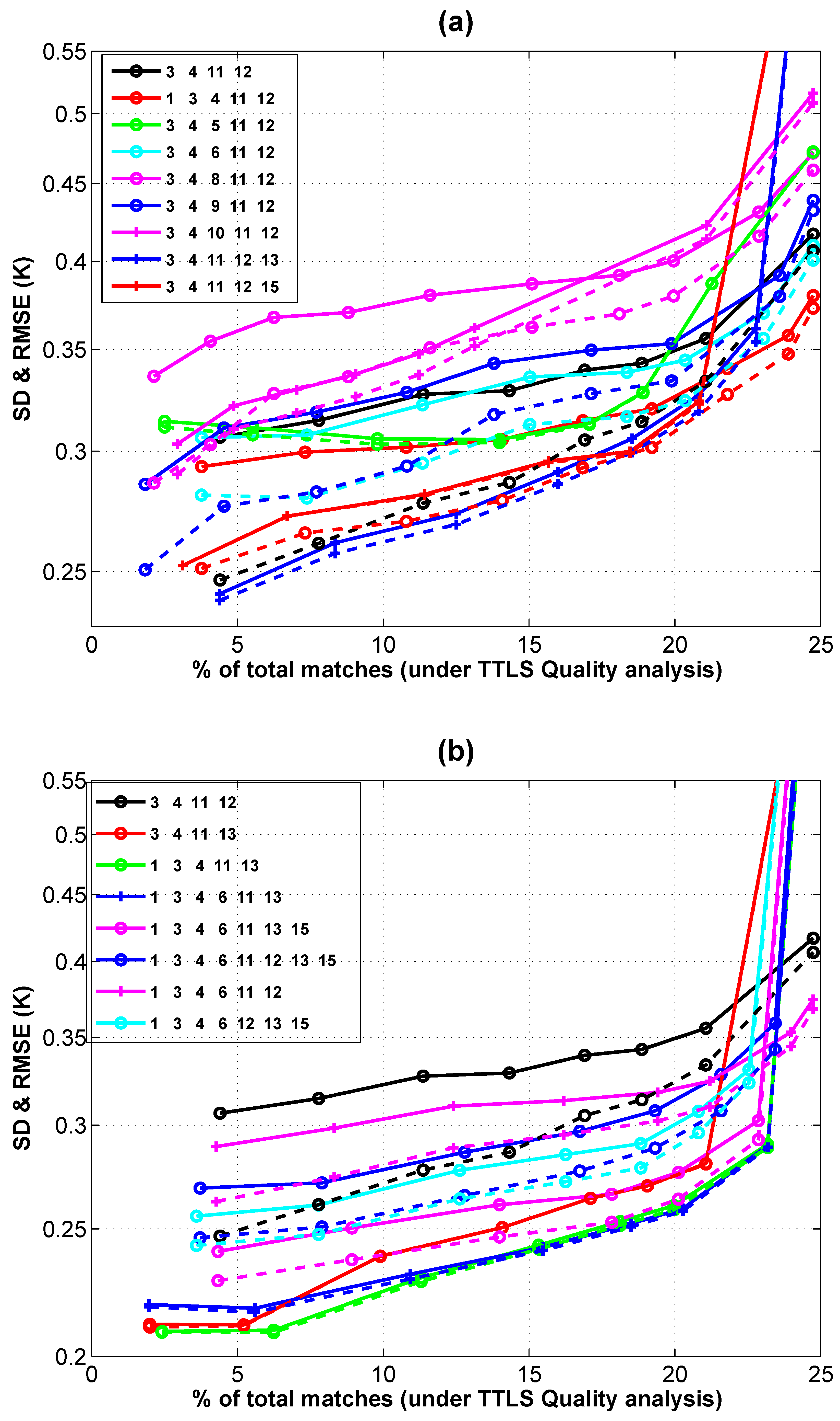
From a deterministic point of view, it is always better to use more measurements for any physical deterministic retrieval, in order to reduce the effects of measurement noise and errors in parameters and missing parameters, if an adequate forward model is available. Due to operational constraints, we have to use the fast forward model (CRTM v2.1), where two types of noise are injected into the inverse problem: (a) approximated RT error and (b) error due to erroneous or lack of ancillary data. To understand and verify the useable channels of MODIS for SST retrieval under the constraints of fast forward model error, we conduct a comparative retrieval, using different channels combinations, as shown in Figure 1. The center wavelength of the sixteen bands of MODIS are 3.7, 3.95, 3.95, 4, 4.45, 4.5, 6.7, 7.3, 8.55, 9.7, 11, 12, 13.4, 13.65, 13.9, and 14.2 μm. Note that the two channel numbers for 3.95 μm are for two different spatial resolutions. The channel number is used in Figure 1 according to this sequence. Most of the prevalent MODIS SST retrievals are made using 3.95, 4.0, 11 and 12 μm channels (Sequence number 3, 4, 11 and 12), which is considered the default combination for this study. We add additional channels (except water vapor channel 7), on top of the default combination for each experiment, to investigate the CRTM channel errors for SST retrievals from MMDB in July 2015, using TTLS, as shown in Figure 1.

We will primarily discuss all results in this paper based on the value of RMSE; however, we also plot the standard deviation (SD), which is the random error component. The systematic error can be viewed by the separation between SD and RMSE curves, which is governed by either single or combine modeling errors (forward, inverse, and instrument models). We plot RMSE for all figures on top of the SD curve, and, if the latter, is not visible, the systematic error is negligible. This implies that all models are working reasonably well. When the SD curves are visible, there are some systematic errors and it may be necessary to revisit the model components in future work. It is observed in Figure 1a that the error in terms of RMSE enhances, due to the addition of any of channels 8, 9, or 10, for nighttime, as compared to our reference combinations of channels 3, 4, 11 and 12 (black line in Figure 1a). This implies that the fast forward model (FFM) error using CRTM is higher than the information added. Thus, we discard these three channels from the channel-selection scheme for use with the presently available FFM. On the other hand, the RMSE value noticeably reduces, keeping the same SD values when adding the 3.7-μm channel, and the difference between RMSE and SD is negligible keeping the same SD values when the 13.4-μm channel is added. Thus, these two channels, for nighttime, are the focus of our channel selection. Moreover, even though the difference between SD and RMSE is very low, but a large number of pixels are placed into the last bin when channel 5 is added. Thus, we also discard channel 5 from the channel selection scheme. A second experiment is then conducted using combinations of channels 1, 3, 4, 6, 11, 12, 13 and 15, as shown in Figure 1b.

The most interesting result observed in Figure 1b is that the significant retrieval error reduces when the 12-μm channel is replaced by the 13.4-μm channel (red) of the default combination (black line in Figure 1b). The RMSE value except for the last bin is 0.36 K for the default pair and is 0.28 K for the combination of 3.95, 4.0, 11, and 13.4 μm. As per the literature, no prevalent methods have used a 13.4-μm channel for SST retrieval before, except in our previous work on GOES-13. However, MODIS SST retrieval generally uses the regression-based method, and the 12-μm channel is still considered useful to help determine atmospheric effects by differential absorption. This implies that the channel selection for a physical deterministic method is not identical to regression based method. As per the requirement of the regression method, the channels with less water vapor information are the best channels to obtain SST itself, which is somewhat contrary to our physically deterministic method, because the channels with water vapor information are also required, as one of the retrieved parameters is TCWV. The three combinations of channels in Figure 1b yield more or less the same performance; however, in this study we use the combination of 1, 3, 4, 6, 11 and 13 channels for night. The measured BTs for the selected channels are the elements of the y vector in Equations (2) and (5). We observe that the FFM error due to seasonal varying GFS profile error is a major hurdle in physical SST retrieval when using all the available MODIS channels. Thus, the retrieval error, using channels 1, 3, 4, 6, 11, 12, 13 and 15, is significantly higher than for the best combination, which contain only six channels.

4. Comparison of MTLS and TTLS

Accounting for the effects of aerosol is one of the major concerns for improving the quality of SST [35,36]. There is no scope to mitigate this issue directly in regression equation based SST retrieval schemes, except discarding pixels from the datasets using additional tests, or simple post hoc bias correction [36], which will reduce the data coverage. There are two choices in the physical based retrieval method to mitigate this issue. Either the aerosol forecast data can be simply treated as “truth” in the forward model, or these data can be used as an initial guess, and an aerosol term can be added to the retrieved parameters. 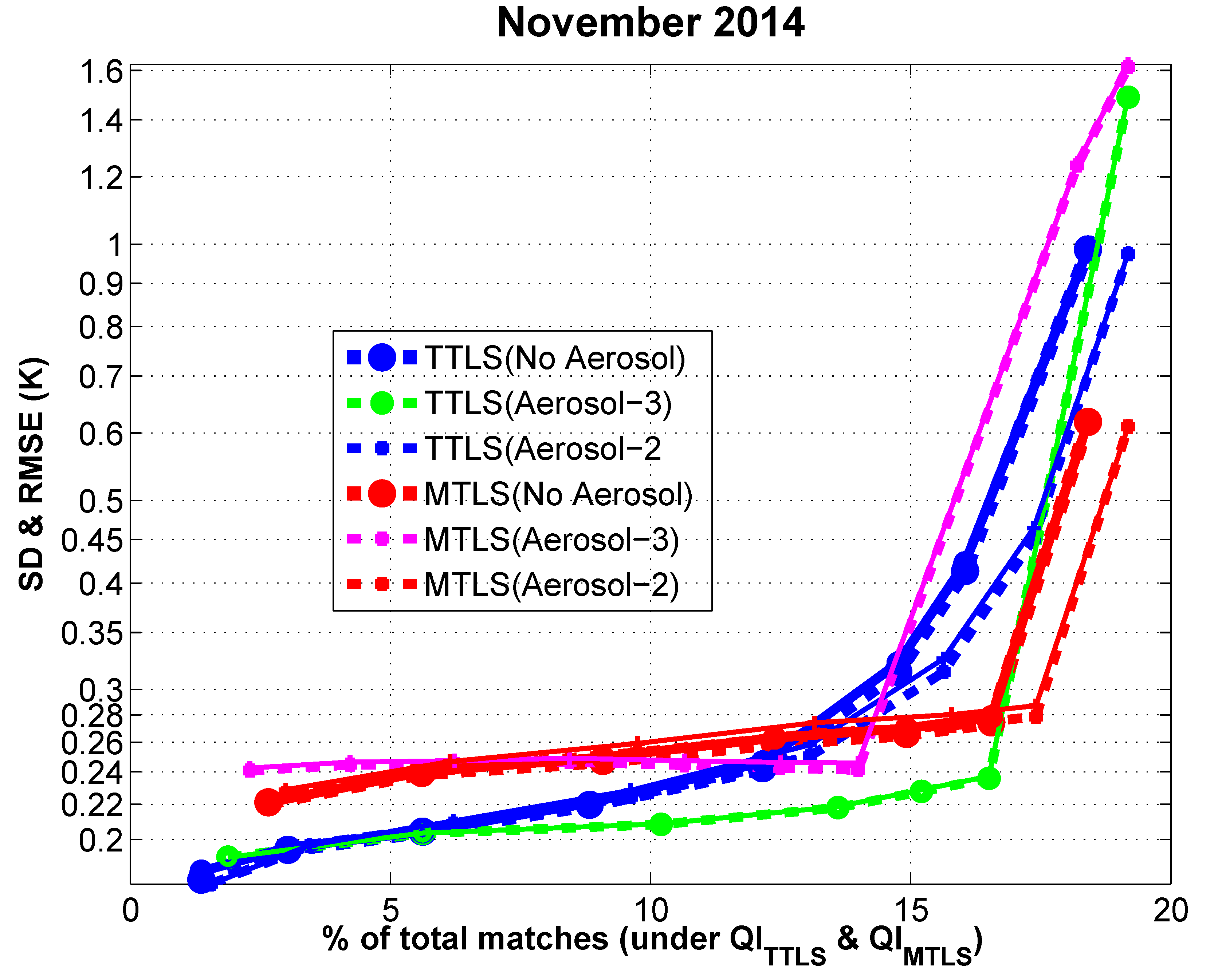We have compared results (Figure 2) for three different scenarios: (a) without ancillary aerosol information; (b) with aerosol but not included as a retrieval parameter; and (c) including a retrieval parameter of total aerosol column density (TACD). In the latter two cases, NGAC provides additional input to the CRTM. We have chosen the MMDB of different months for various experiments to exhibit the versatile characteristics of retrievals, which cannot be viewed from time series analysis based only on the RMSE value.

Figure 2 shows that the retrieval performance of SST is very slightly worse than without including aerosol in forward model simulation for both methods of MTLS and TTLS, but data coverage increase for both cases. This implies that aerosol content from NGAC should not be regarded as a true quantity from a deterministic understanding at the pixel level. In the comparison of MTLS and TTLS, using two retrieved parameters (SST, TCWV) for the whole dataset (except the last bin), the RMSEs of TTLS (0.42 and 0.46 K) are higher than for MTLS (~0.28 K), and data coverage are also reduced for cases, both with and without aerosols. As we discussed in an earlier publication [28], for two parameters, the TTLS retrieval is a highly regularized solution to the inverse problem, and the retrieval error is increased due to a relatively high regularization error. This prompted us to design the new regularized TLS method, MTLS, for cases when the available number of measurements is low. However, the RMSE of TTLS is improved using QI of TTLS for a subset of the whole dataset, e.g., the RMSE of TTLS and MTLS with aerosol are 0.22 K and 0.24 K for the best 8% of matches, respectively (i.e., about 44% of the cloud-free data). Interestingly, both RMSE of MTLS and TTLS are increased due to inclusion of NGAC aerosol in the forward model. On the other hand, SST retrieval using TTLS is significantly improved when we consider the NGAC aerosol profile as an IG for a retrieved parameter of TACD, and data coverage is also slightly improved, as compared to other two scenarios. The RMSE of MTLS with three parameters is 1.2 K, except the last bin, but the RMSE reduces to ~0.24 K except the last two bins. As already mentioned, MTLS was originally designed for a two parameter retrieval scheme, where the number of measurements is limited and constrained by the condition number of the Jacobian. The condition number of the Jacobian is inherently increased due to an increase in the number of retrieved parameter and the population of the “last but one bin” increased due to a high SST error from the resulting high regularization error. Thus, only a two parameter MTLS with aerosols in the forward model can increase data coverage of 1.5% (i.e., about ~9% of the cloud-free data) at a cost of an increased RMSE of ~0.02 K, which is expected to be a better choice for MTLS implementation and is considered in the next experiment. The best results found from this study are that an RMSE of ~0.24 K, with a data coverage of 16.5%, using the three-parameter TTLS retrieval. We have excluded the upper portion of the figure, because the results for the pixels consigned to the “last bin” are not relevant to this study.

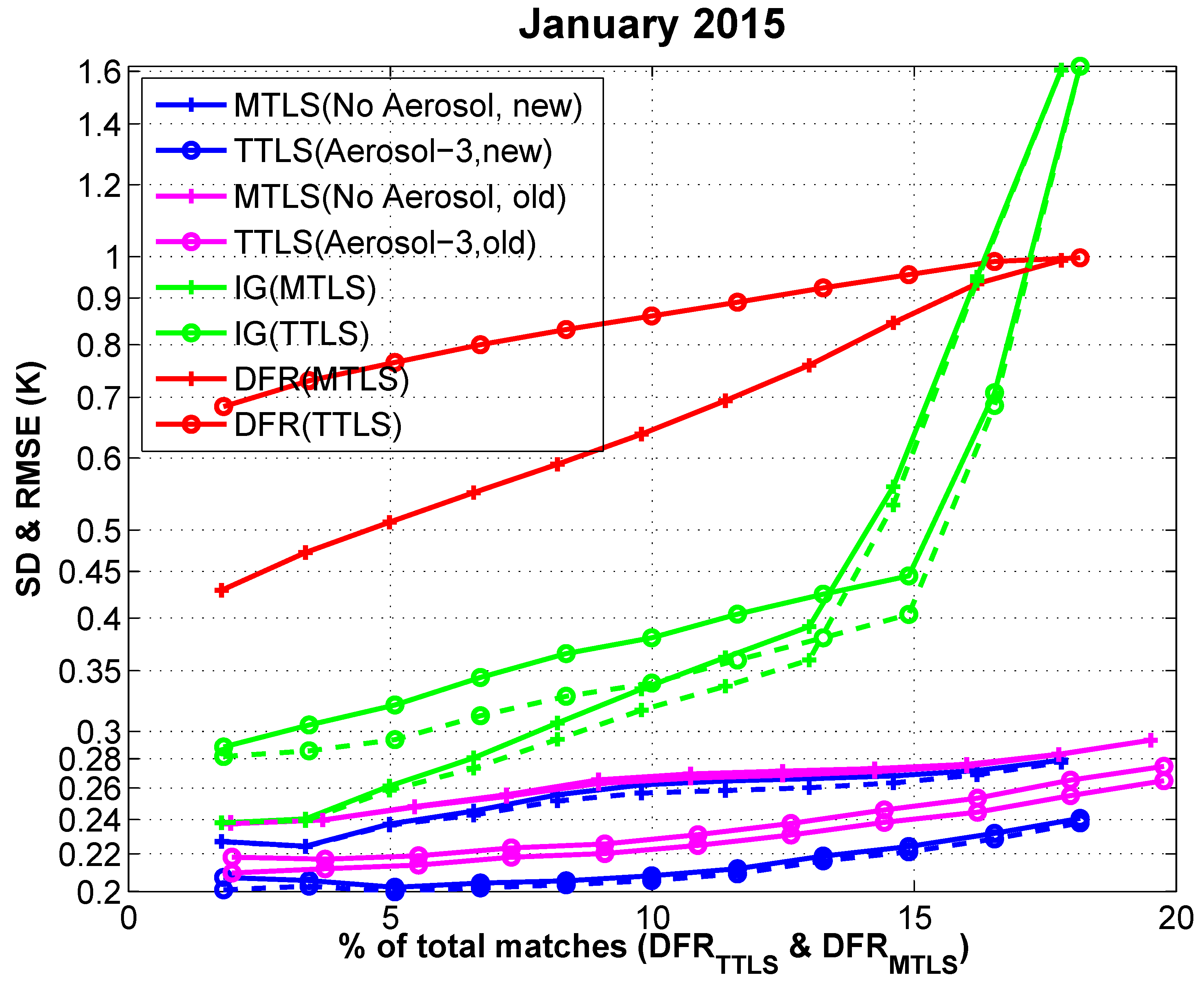
Figure 3 illustrates a comparison study for the three-parameter TTLS and two-parameter MTLS retrievals with aerosol, using the MMDB of January 2015. This study has been made to understand the information content of various retrievals, and Figure 3 has been plotted with the cumulative percentage of total matches, according to the DFR metric for TTLS and MTLS. Although DFR, according to Equation (4) is the ‘trace’ of $M_{rm}$, which is the total information content, we consider first diagonal component of $M_{rm}$ in this study as only the DFR of SST. Figure 3 shows that the three-parameter TTLS retrieval is better in terms of a low error in retrieval and a high value of DFR. Even though it is not really an essential requirement to have high information when a priori error is low, the information content, in terms of DFR, is rather low (<0.45) for the MTLS two-parameter retrieval. In contrast, the TTLS three-parameters retrieval is a better choice when the number of measurements is sufficiently high. On a separate note, we have reported [37] that the DFR value of MTLS is less than 0.3 for the same experiment using data from a different month. The low value of DFR for MTLS is not principally caused by the use of data from a different month; rather, it was due to the tuning of the MTLS implementation in earlier work. We observed that the overall condition number of the Jacobian for a six-channel MODIS SST retrieval is significantly higher than for a three-channel GOES-13 SST retrieval. To improve the performance, we intuitively increased the regularization strength using the MTLS tuning parameter ${\gamma }_{snr}$. The increased regularization strength has highly impacted the information content of the retrievals. Thus, we implemented MTLS for this study in exactly the same way as it was developed for GOES-13. Figure 3 also compares the MTLS and TTLS retrievals for two different proposed thresholds of EXF. Previously [32], we assumed a 1 K threshold and empirically modified the thresholds (0.75/K_3.9) in this paper. The range of RMSE of TTLS, under new threshold of EXF (blue line in Figure 3), is 0.24 to 0.20 K, which is close to the inherent ‘buoy’ error, as reported previously [12]. This also implies that the improved empirical threshold for EXF is justifiable to get very close to complete cloud-free conditions.

5. Cloud and Error Masking

EXF assists in algorithm design and performance studies of the cloud-free retrieval models and the verification of cloud detection schemes. However, it cannot be implemented in operations because in situ measurements are not available for all satellite pixels. We have already reported [32] a novel cloud and error-masking (CEM) algorithm, using both functional spectral differences and RT-based tests for GOES-13 for operational use. As we previously reported [32], the threshold test of the spectral differences of 6.7 and 11 μm for GOES13 is a function of TCWV. However, the RT function (transmission) is significantly dependent on the shape of the profiles, and can be better approximated using an SST Jacobian value of 12 μm. Moreover, as we reported [32], 50% of the forward model calculations are not required if TCWV-dependent spectral difference tests are applied, but this benefit is not achieved in reality for a full-swath of image data, as opposed to matchups. The reason is that the forward model calculation is made at the resolution of the NCEP grid (0.5° × 0.5°), which covers ~2500 pixels (nadir viewing), and if only 100 measurements are cloud free, we still need the forward model calculations for implementing physical retrieval methods. Thus, we have modified the spectral differences tests, based on the SST Jacobian value of the 12-μm channel ($K_{sst}^{12}$). The improved CEM for MODIS is as follows:

$$\frac{2\left(T_{11}^m-T_{6.7}^m\right)}{T_{11}^m+T_{6.7}^m}>0.08+\frac{1-{({\mathrm{K}}_{sst}^{12})}^{0.5}}{10}$$

(6)

$$\frac{2\left(T_{11}^m-T_{13.4}^m\right)}{T_{11}^m+T_{13.4}^m}>0.02+\frac{1-{({\mathrm{K}}_{sst}^{12})}^{0.35}}{10}$$

(7)

where $T_a^m$ stands for the brightness temperature of a MODIS-A measurement for channel “a”. The other tests, namely the functional spectral difference tests of 3.9- and 11-μm channels, the double differences test between channels 3.9 and 4 μm, the water vapor threshold filter (WVTF), and the spatial homogeneity test, are kept exactly same as has been reported [32]. The coefficients for the empirical Equations (6) and (7) are determined using the MMDB from July 2014, and these have been used for different months.

6. Validation

As mentioned earlier, to compare our SST retrieval with available operational MODIS SSTs, we have downloaded data from the GHRSST website. The database contains two operational MODIS SST products (short-wave and long-wave) with ancillary information, quality levels (MQL) from 1 to 5 (for bad to good retrievals), for the two different SST products. We anticipated that the cloudy pixels would be discarded using a cloud detection algorithm, and then the SST quality level is assigned according to the performance of the retrieval algorithm in operation. It is not unreasonable to expect that a quality level of 3 and above from the operational database as representative of the total cloud-free pixels obtained from the MODIS cloud (MC) algorithm for the comparison of our cloud scheme. However, it turns out that two subsets of pixels (MQL ≥ 3) for two different products are significantly different. The reason for the substantial difference in QL = 3 data between the long-wave and short-wave SST products in MODIS is not immediately obvious, because the tests are essentially the same (see http://oceancolor.gsfc.nasa.gov/cms/atbd/sst/doc/html/flag.html). However, one possibility is that the spatial uniformity test degrades all long-wave MODIS SST data by one quality level, however, this does not appear to be applied to the shortwave MODIS SST product. Thus, long-wave MODIS SST data, which were originally GHRSST QL = 3, may have been degraded to QL = 2. As we are comparing the partition of data by quality level, and the effects of cloud contamination, and we previously reported [25] that the subset of pixels (MQL ≥ 3) from short-wave data base contains substantial cloud leakage, we consider the subset of pixels (MQL ≥ 3) from the long-wave database is actually representative of MODIS cloud (MC) to compare the performance of our newly developed cloud algorithm.

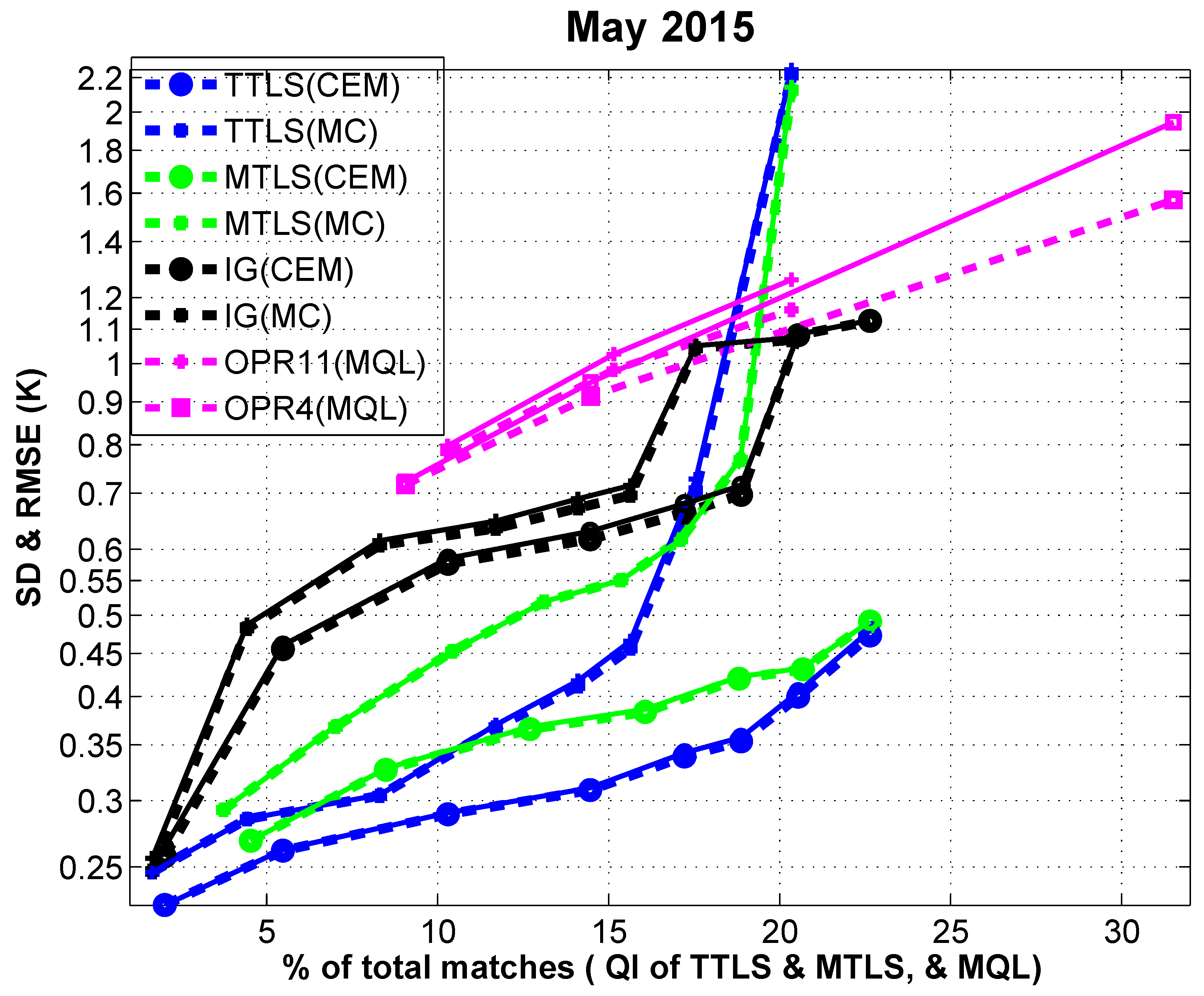
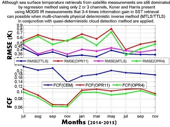
We first show a detailed discussion to results for the month of May 2015, to understand, in depth, the characteristics of different retrievals, while time series results will be presented in Section 7. The retrieval errors for two different deterministic methods (TTLS with three parameters and MTLS with two parameters) and two operational products (OPR4 and OPR11) under two different cloud detection schemes (CEM and MC) are shown Figure 4. The errors in SST retrieval are shown in Figure 4 using two different metrics: (a) root mean square error (RMSE) and (b) standard deviation (SD). As we mentioned earlier, RMSEs are plotted over the SDs—when the lines merge (i.e., the dashed SD line is not visible), the systematic error component of RMSE is negligible. The new cloud detection scheme, CEM, classifies ~1.8 times more pixels as cloud-free (i.e., able to obtain a good SST estimate) compared to the MQL = 5, for long-wave, and ~2.1 times more than the same MQL = 5 for short-wave. Note, however, that the standard MODIS cloud-free or highest quality level pixels are not simply a subset of our set. Figure 4 shows that the RMSE of OPR11 and OPR4 for a QL of 5 are ~0.79 K and ~0.72 K, and only comprise ~10% and ~9% of the total number of matchups, respectively. On the other hand, CEM classifies ~18.9% of all pixels in the matchup dataset as cloud free (except the last bin), with an RMSE of TTLS of ~0.4 K. This represents more than a three-fold information gain in terms of low error and high data coverage using the combination of CEM and TTLS. It is worth mentioning that the highest quality of TTLS retrieval of 5%, with respect to total matchups (i.e., ~25% of the cloud-free observations), is 0.25 K, which is again comparable with buoy errors. The data coverage of operational MODIS SSTs can be increased to ~20% by reducing the quality level to 3 (long-wave), but with a concomitant increase of RMSE to ~1.25 K. The information gain for CEM+MTLS remains at more than three times, even if we consider the threshold of cloud at MQL ≥ 3 (long-wave). It is also observed from this figure that the IG error for whole cloud-free dataset in CEM is comparable to the same under the group of MODIS cloud free (MQL ≥ 3, long-wave) pixels, which eliminates the possibility that CEM is only selecting the pixels with SSTs close to the IG.

Although MTLS and TTLS are the same family of deterministic TLS methods, the results are not similar, due to data-driven regularization being determined using different procedures. As observed in Figure 4, there are significant differences in results under both cloud schemes. TTLS is always superior to MTLS under CEM, but there is an intersect for the MC regime, due to the fact that MTLS (excluding last bin) increases the data coverage by 1% at the cost of an increased RMSE of 0.05 K. However, the overall performance of TTLS is better than MTLS, as intended. Even though the improvement of TTLS over MTLS is fairly modest (0.05~0.1 K), both MTLS and TTLS are far better than the performance of both operational short-wave and long-wave products. On the other hand, the data coverage (except the last bin) of MTLS and TTLS are more or less equal (20.54% and 20.68%) under CEM. Both MTLS and TTLS show an excellent performance to remove the additional cloudy pixels at the time of solution, which can be observed from RMSE curves of MTLS and TTLS under MC. The RMSEs of TTLS and MTLS reduce from 2.2 K and 2.1 K to 0.72 K and 0.77 K for data elimination of 2.8% and 1.5%, respectively. This confirms that the additional cloud removal using TTLS and MTLS solution (last bin) is a useful tool. It should be noted that the reduction of IG error is marginal for both cloud schemes, which implies that high signal SST retrievals are not consigned to the last bin, thus, as mentioned earlier, this version of the algorithm has improved the “last bin” assignment.

While the systematic errors are negligible for both operational products at MQL = 5, they become significant when the quality level is decreased, which is one of the inherent drawbacks of regression methods [28] and the cloud detection problem. To remove systematic errors in an operational setting requires a dynamic coefficient evaluation procedure, which may increase the total errors. Some noteworthy comparison results (Figure 4) between deterministic- and regression-based retrievals under MC using the TTLS QI are: (a) RMSE values for both MTLS and TTLS are very high (2.1 and 2.2 K) for quality level 3 (long-wave) but, after “last bin” cloud removal, the RMSE of MTLS and TTLS are 0.72 and 0.77 K, which are lower than OPR11 (0.79 K) at MQL = 5; (b) the data coverage for MTLS and TTLS increases from 10% to ~18.5% (85% increasing data coverage with respect to operational) and from 10% to ~18% (80% improvement), respectively for the equivalent RMSE value of OPR11 at QL = 5 (0.79 K), when extending the sample of operational SST retrieval pixels to include MQL ≥ 3; (c) the RMSE values of MTLS and TTLS are ~0.45 K and ~0.33 K, respectively, for 10% data coverage (at MQL of OPR11, vertical comparison), while the RMSE of OPR11 is 0.79 K; (d) The RMSE of OPR4 (0.72 K) is slightly better than for OPR11 at MQL = 5, but the RMSE of TTLS for the same data coverage is ~0.32 K; (e) all other comparison between OPR4 and deterministic retrievals (MTLS and TTLS) are similar to those for the OPR11 and deterministic retrievals.

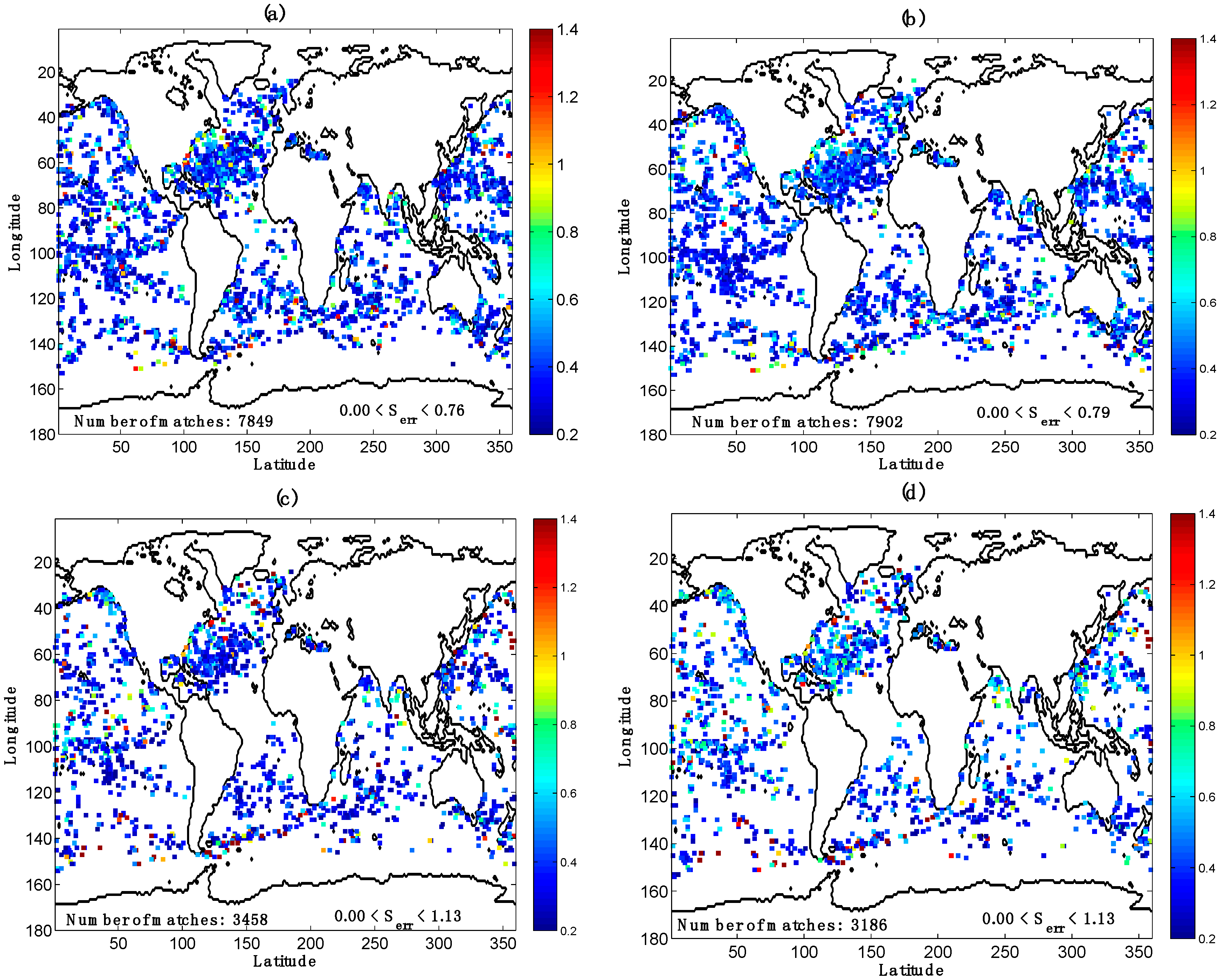
To illustrate the geographical error distribution, the absolute difference between the retrieved SSTs from the corresponding buoy measurement at a finer grid of 0.05° × 0.05° lat/lon is obtained, and we calculate the RMSE value of the differences if any grid has more than one match-up using MMDB for May 2015. We confined this study to a fine grid in order to allow for comparison of both accuracy and data coverage of different retrieval and cloud detection schemes. It is challenging to discern the exact error distribution by the human eye when errors are mapped at the fine-grid level, thus, we have calculated the spread of errors (S_err) in terms of a geographical view for the comparison of different products. This was calculated by keeping the minimum value unaltered and the maximum value is determined by sorting the lowest 95% of data. The errors of four different products are mapped in Figure 5. We have not identified any specific trend of the error distribution for any products with respect to a particular geographical location, but the reduced data coverage of the two operational products is easily discerned. The red spots in all maps are probable cloud contamination. It is not sensible to calculate a systematic error when the number of points is less than 10, and more than 95% of pixels have less than this. Surprisingly, the value of S_err for both operational products is same (1.13 K), the reason for this is not clear. The values of S_err for MTLS and TTLS are 0.79 and 0.76 K, respectively. Figure 5a,b also demonstrates that CEM can improve the data coverage at high latitudes, which is highly desirable for many geoscience problems.

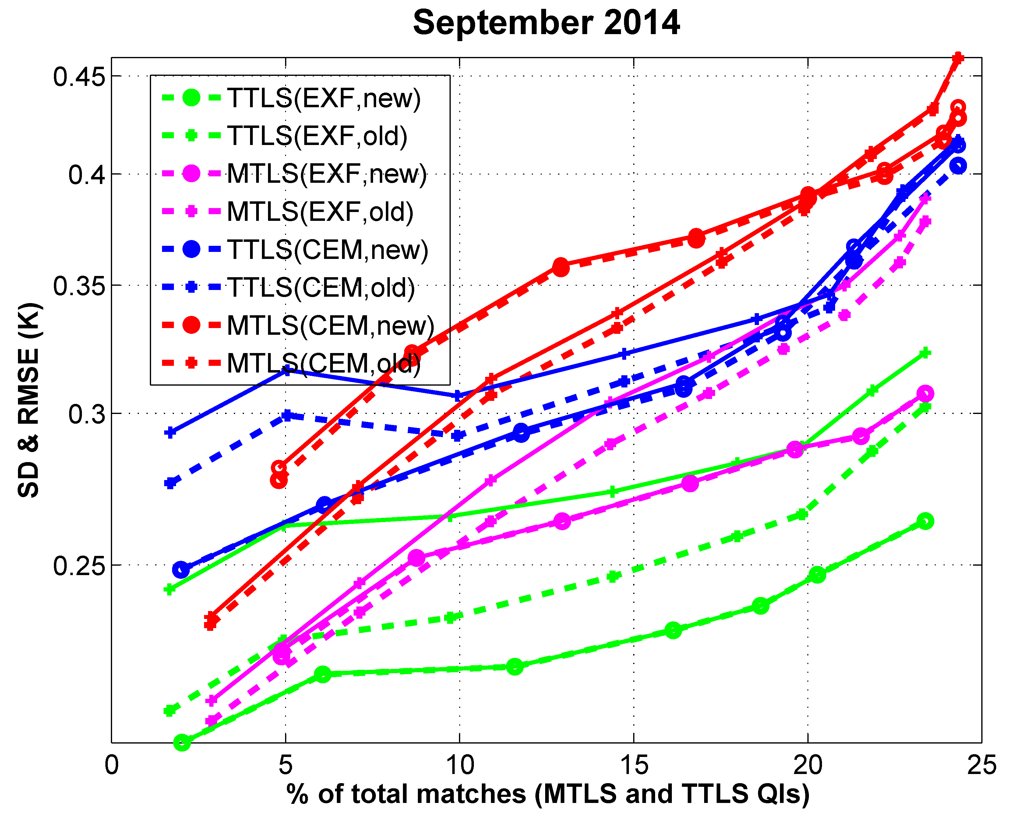
One may observe that the selected channels in this study are not the same as our previous study [25]. To maintain consistency with our earlier report, we have made an experiment using the previously selected channels and those in the present work under CEM and EXF, as shown in Figure 6. It can be seen from these results that there are no systematic errors evident for all retrievals (MTLS and TTLS) under both CEM and EXF when the newly selected channels are used, but there are significant systematic errors for all above-mentioned retrievals, except for the combination of MTLS+CEM, using the old channels. Moreover, the RMSEs of all retrievals for the newly selected channels are lower than those for the previously-selected channels, again, except for the case of MTLS+CEM. As the RMSE of MTLS+EXF retrieval is lower in new selection, as compared to the old selection, including for both TTLS retrievals, this confirms that the new channel selection is the better choice. This infers that a systematic channel selection procedure using EXF is the best approach, since it allows for the separation of cloud detection and retrieval aspects. In our earlier work, the channel selection was made intuitively, with some empirical tests, which resulted in a sub-optimal selection. However, the RMSE of MTLS+CEM, between the old and new selections, is closer and the curves do intersect; thus, the impact of employing the previous selection is by no means disastrous. Moreover, when at least one channel from ~4 um window, one channel from 8–12 um window, and one channel from LWIR are considered, it will produce good SST retrieval, using any appropriate physical deterministic retrieval, assuming the forward model is moderately accurate.

7. Time Series Analysis

To achieve more confidence in the deterministic TTLS method for MODIS SST retrievals, we have analyzed more than a million match-ups over a period of more than a year, and these results are shown in Figure 7. The superiority of the TTLS method over the regression based MODIS SST, drawn on the basis of one month’s analysis, also holds for this longer time series, implying that the gains from the TTLS methodology are temporally robust. The average values of RMSE and data coverage for TTLS+CEM are 0.35 K and 19% (where fraction of cloud free (FCF) pixels is 0.19), for OPR4 (MQL = 5) are 0.52 K and 8.8%, and for OPR11 (MQL = 5) are 0.57 K and 9.7%. The reduced data coverage of OPR4, compared to OPR11, is mainly caused by data availability. We made this calculation based on the total match-ups for night, and we found in the database that OPR4 data are not available if the granule is mixed day and night, but OPR11 data are available. The average information gain using TTLS+CEM is also more than three times that of OPR4 and/or OPR11. A large RMSE variation from 0.72 K to 0.34 K (>100%) over a period ten months is observed for OPR4 products, whereas the values of RMSE for TTLS+CEM are fairly consistent from 0.43 K to 0.33 K. The RMSE of OPR4 is surprisingly low (0.34 K) for the month of July 2015, thus, perhaps, some overhauling of the algorithm was performed, although the improvement seems to have been only temporary. Even though the RMSE of OPR4 is lower than that of TTLS for the month of July 2015, the data coverage for TTLS+CEM for this month is almost double than that of OPR4, at MQL = 5. It is difficult to conclude from these results whether or not there is significant seasonal dependency of the RMSE of the operational products—further investigation is likely to require a longer time series. The RMSEs of OPR4 (except for November 2014) are lower than those of OPR11, thus, it can be conclude that OPR4 is a better product than OPR11. Even though the improvement of TTLS over MTLS is not large, the information content of TTLS is always significantly higher than MTLS, which was discussed earlier.

8. Conclusions

This study shows that the performance of the deterministic inverse method of TTLS is better than that of MTLS when more measurements are available. The number of retrieved parameters is constrained by the number of measurements for any inverse modeling and increased parameter retrieval is possible when more measurements are available. TTLS solutions, exploiting more channels, as compared to conventional SST approaches, are always better than the prevalent regression methods under consideration when using different cloud detection schemes, and also cope well with various operational constraints. The additional cloud detection and quality flagging using the analytic error calculation at the solution time of TTLS is fully objective, and results display compliance with in situ validation and additional cloud masking. In summary, this work introduces the following advances compared to previously published work: (a) a new method of truncated total least squares; (b) incorporation of explicit aerosol information in a forward model; (c) addition of an aerosol component to the inverse model; (d) a methodology for channel selection; (e) information content analysis for MODIS SST retrieval; (f) a better empirical threshold for EXF; (g) improvements to the CEM algorithm; and (h) time series error statistics for physical MODIS SST.

The operational SST products available from the GHRSST website do not appear to be optimum, in terms of quality and data coverage. The TTLS algorithm, in conjunction with CEM, as well as quality indexing at the individual pixel level, should improve the situation. MODIS-derived SSTs have many applications in atmospheric and oceanic studies, and with more than a decade and a half of continuous data availability, they form a tremendously important part of the geophysical record. An increase of ~3× information content, when compared to the operational available MODIS SSTs, demonstrated using a month of match-ups and was confirmed by the time series analysis, should open up a new frontier in a variety of geophysical applications.