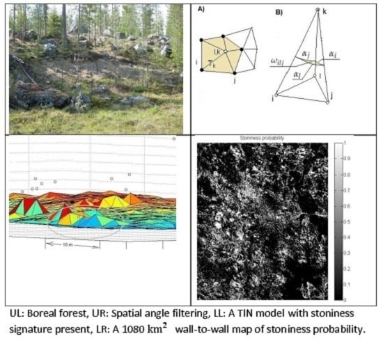
Article

Detecting Terrain Stoniness From Airborne Laser Scanning Data † †

1
Department of Information Technology, University of Turku, FI-20014 Turku, Finland
2
Geological Survey of Finland, P.O. Box 77, Lähteentie 2, 96101 Rovaniemi, Finland
*
Author to whom correspondence should be addressed.
This paper is an extended version of our paper published in Paavo Nevalainen, Ilkka Kaate, Tapio Pahikkala, Raimo Sutinen, Maarit Middleton, and Jukka Heikkonen. Detecting stony areas based on ground surface curvature distribution. In The 5th International Conference on Image Processing Theory, Tools and Applications, 2015.
Remote Sens. 2016, 8(9), 720; https://doi.org/10.3390/rs8090720
Submission received: 29 June 2016 / Revised: 7 August 2016 / Accepted: 17 August 2016 / Published: 31 August 2016
(This article belongs to the Special Issue Airborne Laser Scanning)

Abstract

:
Three methods to estimate the presence of ground surface stones from publicly available Airborne Laser Scanning (ALS) point clouds are presented. The first method approximates the local curvature by local linear multi-scale fitting, and the second method uses Discrete-Differential Gaussian curvature based on the ground surface triangulation. The third baseline method applies Laplace filtering to Digital Elevation Model (DEM) in a 2 m regular grid data. All methods produce an approximate Gaussian curvature distribution which is then vectorized and classified by logistic regression. Two training data sets consisted of 88 and 674 polygons of mass-flow deposits, respectively. The locality of the polygon samples is a sparse canopy boreal forest, where the density of ALS ground returns is sufficiently high to reveal information about terrain micro-topography. The surface stoniness of each polygon sample was categorized for supervised learning by expert observation on the site. The leave-pair-out (L2O) cross-validation of the local linear fit method results in the area under curve A U C = 0 . 74 and A U C = 0 . 85 on two data sets, respectively. This performance can be expected to suit real world applications such as detecting coarse-grained sediments for infrastructure construction. A wall-to-wall predictor based on the study was demonstrated.

Graphical Abstract

1. Introduction

There is an increased attention towards classification of the small scale patterns of terrain surface. Recognition of micro-topography may help in arctic infrastructure planning [1], terrain trafficability prediction [2], in hydraulic modeling [3], and in detecting geomorphologic features like in [3,4], and terrain analysis and modelling.
In Finland, a nationwide airborne light detection and ranging (LiDAR) mapping program has provided the means for detecting ground objects with the ground return density ρ 0 . 8 m 2 . Since one needs at least one point per stone, and to define the stone radius one needs at least 4 points per stone, this leads to an absolute theoretical detection limit of stone radius r m i n = 0 . 6 . . . 1 . 2 m. The real limit is naturally somewhat higher. The actual stone sizes fall into this critical range (as discussed in Section 2.2) making the stoniness detection a difficult problem.
One aspect of the ground surface is the presence of stones and boulders, which can be characterized by the stone coverage and by stone size distribution. Mass-flow deposits are recognized by irregular distribution of boulders and stones on their surface. Mass-flow deposits may have regional significance in aggregate production if they occur in fields as they do in the Kemijärvi region in Finland. Mass-flow sediments are often moderately sorted sediments with low fine grained fraction (clay and silt content, <0.006 mm) being less than 12 % [5]. In addition they contain boulders and stones in their sediments which may be crushed for aggregates. Therefore, they are potential aggregates for infrastructure construction. Mass-flow deposits can be detected in a two-step process: First candidate polygons are found by analyzing geomorphological features in a process which can be automated, then surface stone detection based on airborne LiDAR data is performed to limit the set of candidates. Various other geomorphological features like paleolandslides [6], fluvial point bars [7], neotectonic faults [3] and Pulju moraines [8] in Finland and several other types of glacial landforms elsewhere (see summary in [9]) have already been mapped using LiDAR data.
The intent of this paper is to document various methods, which analyze airborne laser scanning data (ALS) or digital elevation model (DEM) to detect stony areas. Our hypothesis is that a direct approach may be able to detect a signal of a target feature like stoniness better than methods using DEM. This is because DEM is a general smoothed representation of the ground surface for generic purposes [10]. This paper focuses on binary classification of the stoniness of sample areas. The approach results in a classifier, which is subjected to 20 m × 20 m point cloud patches to produce a binary mask about stoniness covering whole Northern Finland. Stoniness is just one example of micro-topographic features, which could be detected from public ALS data. Even the positive samples of the data sets focus on stony mass-flow deposits, algorithms are developed for general stoniness detection, which can be later targeted to various specific purposes depending on the available teaching data. It is our hope that the research community finds our results and methods useful in the future.
This paper is an expansion of [11], which studied only one polygon set data2014 using curvature estimation based on local linear fit (LLC). In comparison to [11], this paper uses an additional data set data2015, additional public DEM data format and two additional methods: local curvature estimation based on triangulated surface model computed from LiDAR (LTC) and Laplace filtering of a DEM grid (DEC). LTC uses triangulated irregular network (TIN) produced by a solid angle filtering (SAF). An overview of the relation of computational methods and various data formats can be seen in Figure 1.
The structure of the paper is as follows: a summary of current research applicable to micro-topographic feature detection is in Section 1. Data sets and data formats are explained in Section 2.2. The solid angle filtering (SAF) can be used by two presented methods, it has been described in Section 2.4. Three methods are documented in Section 2.5, Section 2.6 and Section 2.7. Methods are compared in Section 3. Possible improvements are discussed in Section 4 and further application areas considered in Section 5.

Current Research

A good presentation of general-purpose ALS classification is in [12]. Our work relates to some of the contour and TIN -based ground filtering algorithms mentioned in [13], since all of our methods either directly or indirectly use or produce a tailor-made ground model. Methods described in [13] are usually more generic accommodating to infrastructure signatures etc. It is possible, that methods described in our paper have to be combined with existing generic ground model algorithms, where an assembly of methods would use e.g., a voting arrangement at the approximity of constructed environment.
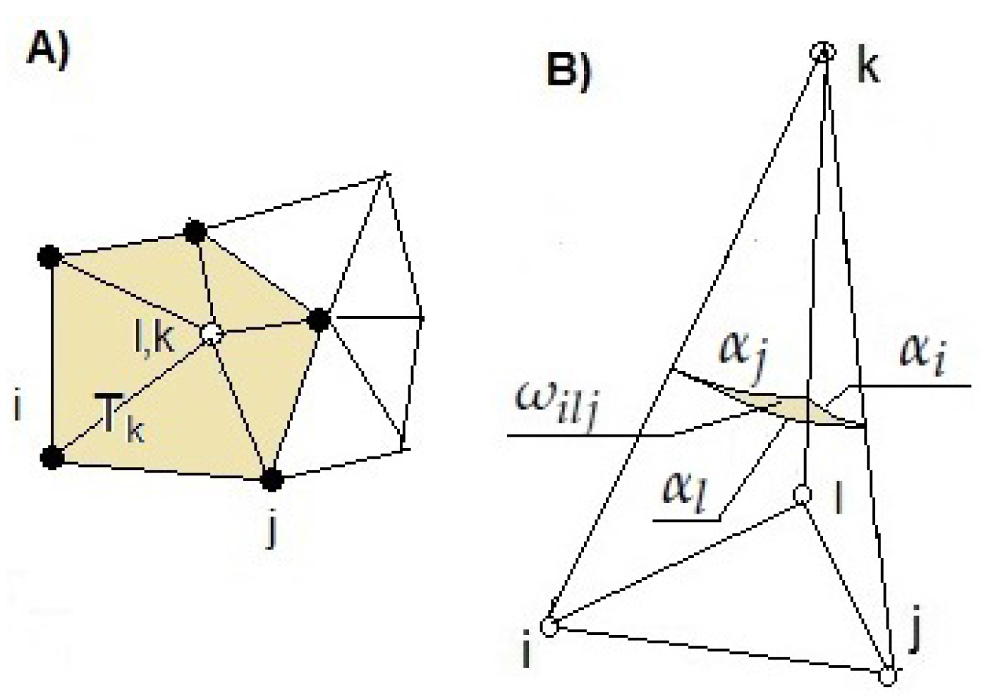
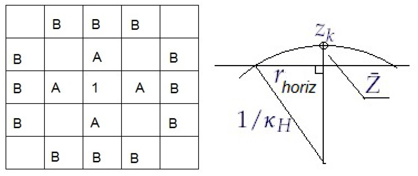
Solid angle filtering (SAF) in Section 2.4 resembles the despike algorithm presented in [14]. Two problems are mentioned in [14]: Unnecessary corner removals (rounding off the vertices of e.g., block-like structures) and effects of negative blunders (false points dramatically below the real surface level). Our routine was specifically designed to eliminate these problems. SAF can also be used in canopy removal. An interesting new technique in limiting the ground return points is min-cut based segmentation of k-nearest neighbors graph (k-NNG) [15]. The graph is fast to compute with space partitioning, and it could have served as a basis for stoniness analysis directly e.g., by fast local principal components analysis (PCA) and local normal estimation with vector voting procedure, as in [16]. The literature focuses mostly on laser clouds of technological environment, where the problem of eliminating the canopy (noise) and finding the ground returns (a smooth technical surface) are not combined. Our experiments with local normal approximation and vector voting were inferior to results presented in this paper. There is great potential in local analysis based on k-NNG, though.
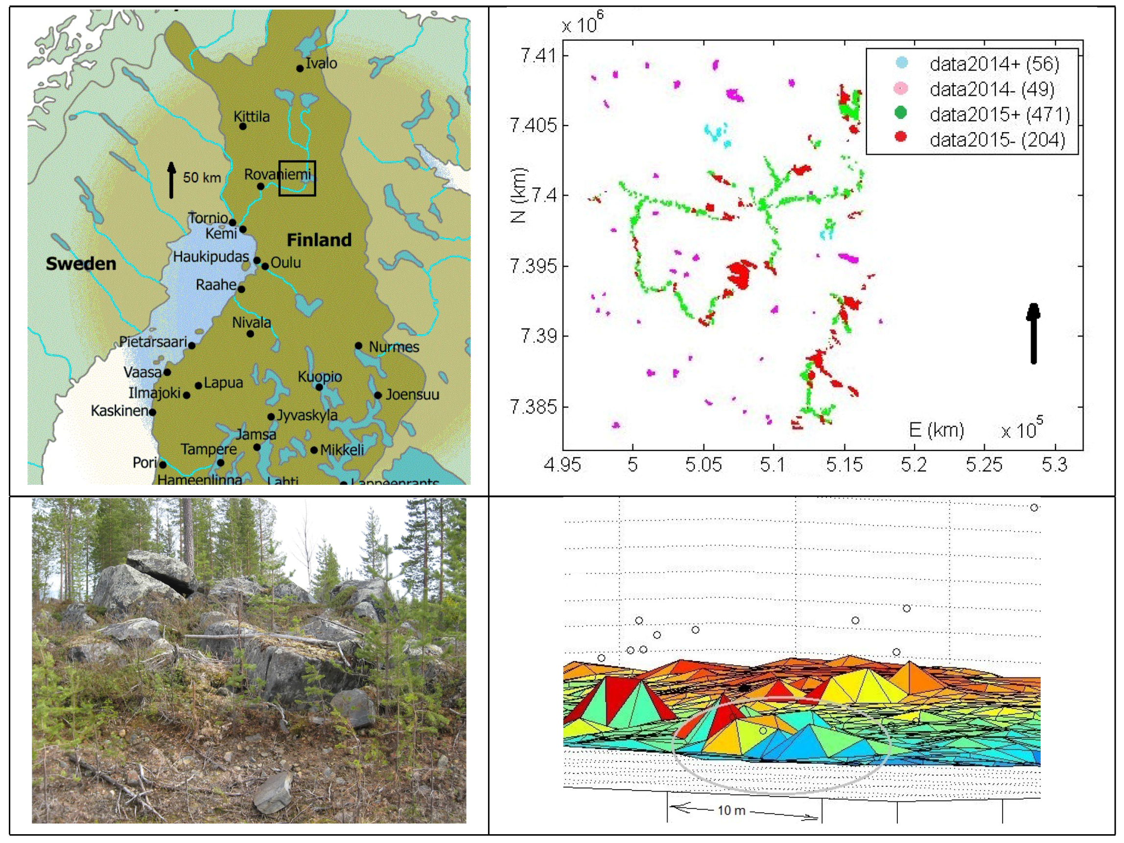
There seems to be no research concerning the application of ALS data to stoniness detection in forest areas. Usually target areas have no tree cover [17], objects are elongated (walls, ditches, archaeological road tracks, etc.) [17,18] and often multi-source data like photogrammetry or wide-spectrum tools are used. curbstones which separate the pavement and road in [18]. Their data has the sample density ρ = 5 / m 2 which produces geometric error of size 0 . 3 m which is larger than the observed shapes (curbstones) and thus not practical. Effects of foliage and woody debris are discussed in [19]. They mention that even a high-density ALS campaign is not able to get a dense sampling of the ground surface in a non-boreal forest (Pennsylvania, U.S.). They reported ground return ratio is 40% with the ground sample density ρ = 4 / m 2 , which is much higher than ρ 0 . 8 / m 2 in our study. The distribution of the local ground sample density was not reported in [19] but is probably much higher than in our case.
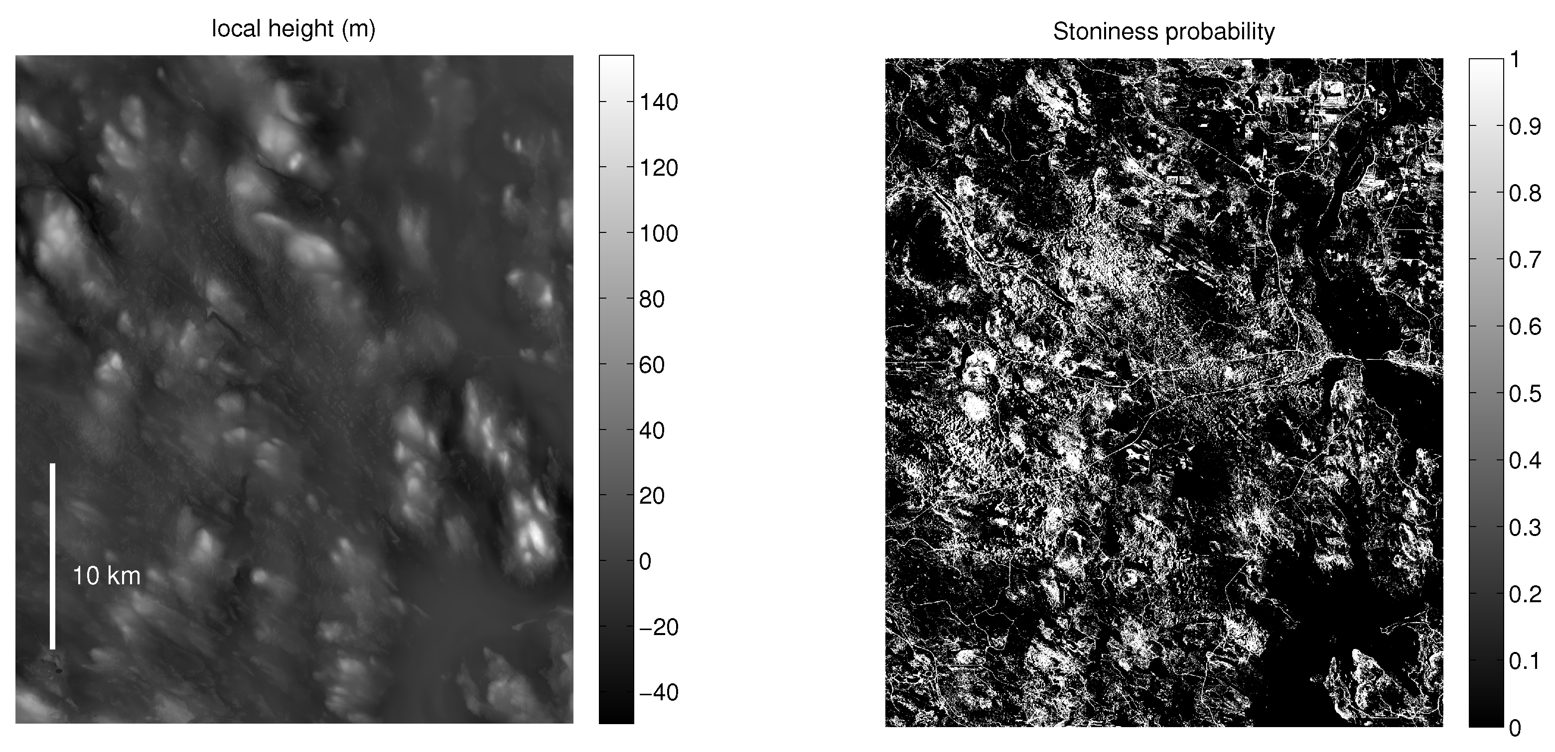
DEM in Figure 1) is a standard data type used by geographic information systems (GIS). Many implementations and heuristics exist (see e.g., [20]) to form DEM from ALS format .las defined by [21]. Usually, the smallest raster grid size is dictated by the sample density and in this case DEM grid size δ = 2 m is possible, and δ = 1 m already suffers from numerical instability and noise.
A rare reference to DEM based detection of a relatively small local ground feature (cave openings) in forest circumstances is presented in [22]. In that paper the target usually is at least partially exposed from canopy and the cave opening is more than 5 m in diameter. On the other hand, the forest canopy was denser than at our site in general. Another application is detecting karst depressions, where slope histograms [23] and local sink depth [24] were used to detect karst depressions. There are similarities with our study, e.g., application of several computational steps and tuning of critical parameters (e.g., the depression depth limit in [23]), although the horizontal micro-topology feature size is much larger than in our study (diameter of doline depressions is 10–200 m vs. 1.5–6 m diameter of stones in our study). The vertical height differences are at the same range, 0.5–1.5 m in our study and in [23,24], though. A similar study of [25] uses higher density LiDAR data with ρ = 30 m 2 to detect karst depressions of size 26 m and more. The vertical height difference (depth) was considerably larger than in in [23,24]. The high density point cloud and a carefully designed multi-step process results in quantitative analysis of sinkholes in [25], unlike in our study, where the stoniness likelihood of a binary classifier is the only output.
One reference [19] lists several alternative LiDAR based DEM features, which could be used in stone detection, too. These include fractal dimension, curvature eigenvectors, and analyzing variograms generated locally over multiple scales. Some of the features are common in GIS software, but most should be implemented for stoniness detection.
Hough method adapted to finding hemispherical objects is considerably slower than previous ones, although there is a recent publication about various possible optimizations, see e.g., [26]. These optimizations are mainly about better spatial partitioning.
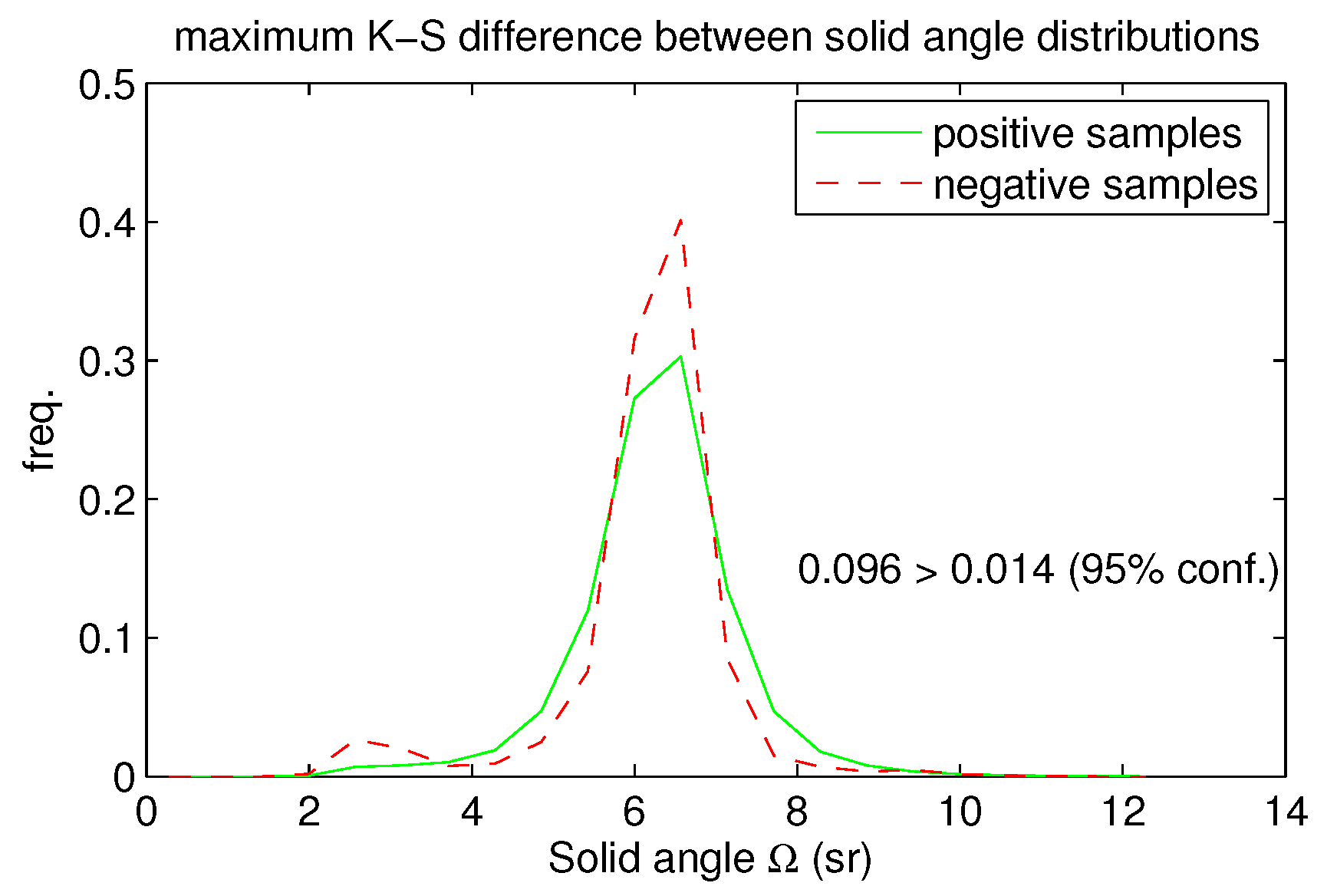
Minimum description length (MDL) is presented in [27] with an application to detect planes from the point cloud. The approach is very basic, but can be modified to detect spherical gaps rather easily. MDL formalism can provide a choice between two hypotheses: a plain spot/a spot with a stone. Currently, there is no cloud point set with individual stones tagged to train a method based on MDL. MDL formalism could have been used without such an annotated data set, but we left this approach for further study. In addition, probably at least 4..8 returns per stone is needed and thus a higher ground return density than is currently available.
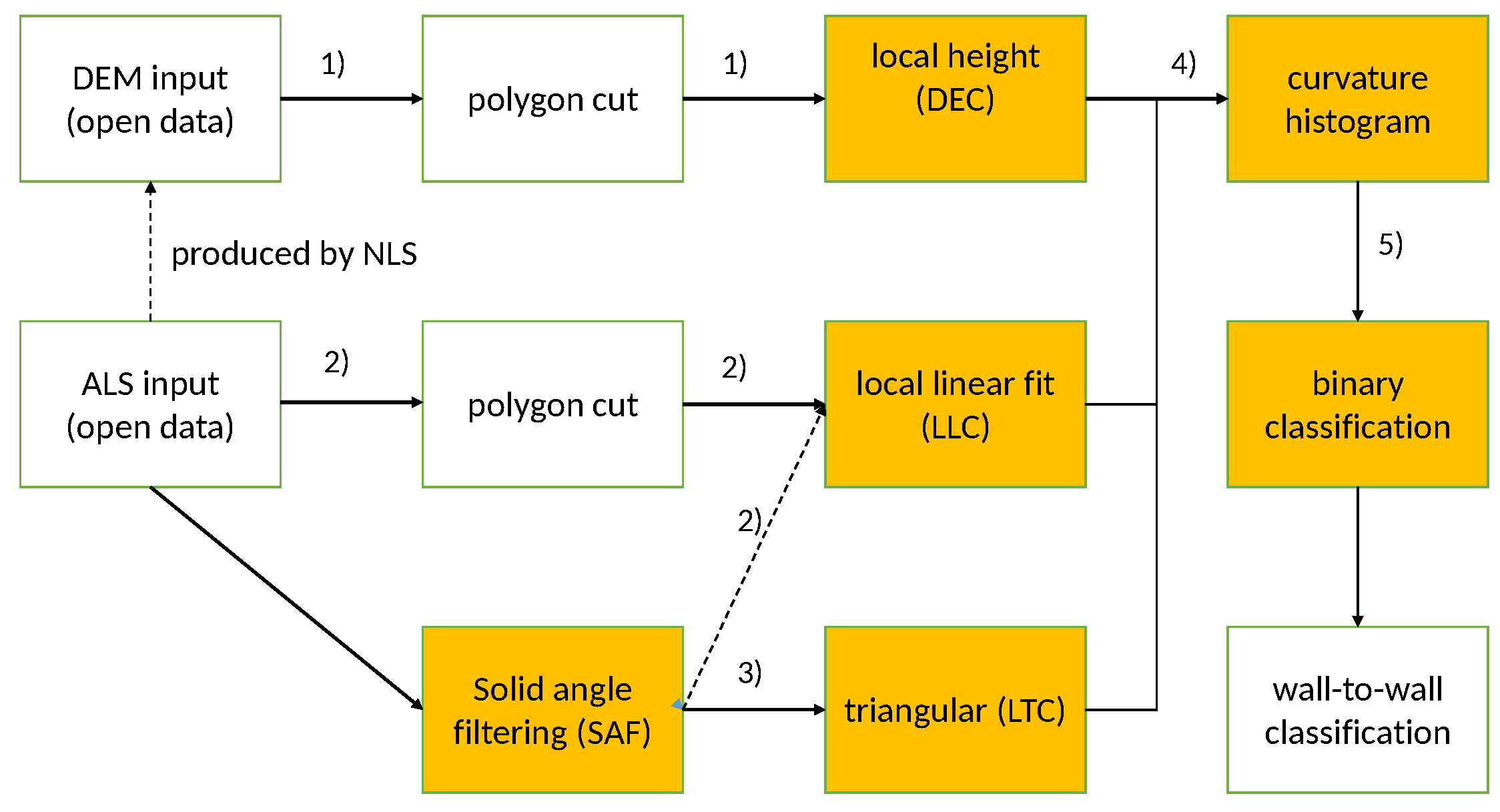
This paper presents two methods based on ALS data and one method using DEM and acting as a baseline method. The DEM method was designed according to the following considerations: It has to be easy to integrate to GIS and it would start from a DEM raster file, then generate one or many texture features for the segmentation phase. The possible texture features for this approach are the following:
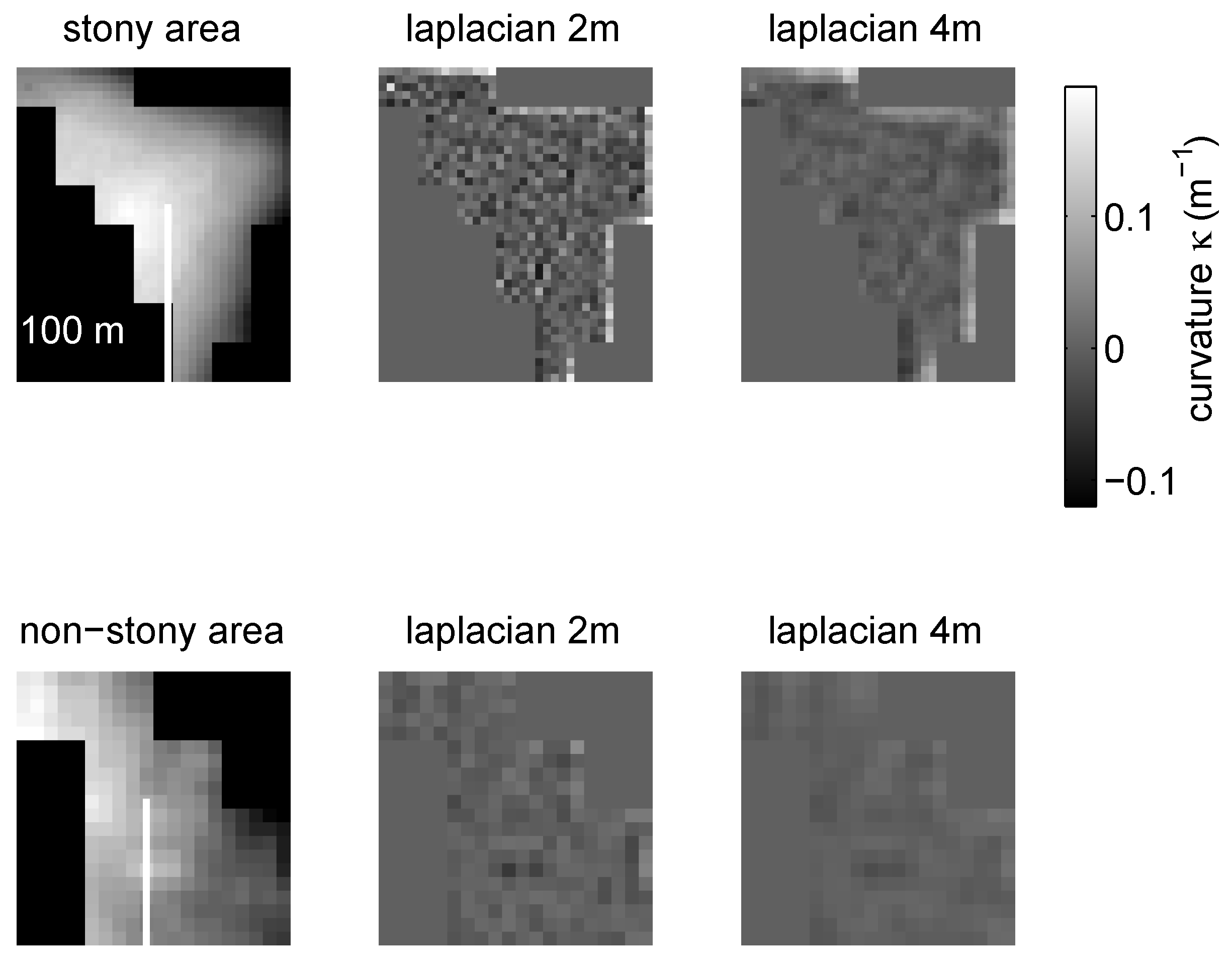
  • local height difference, see Laplace filtering Section 2.7. This feature was chosen as the baseline method since it is a typical and straightforward GIS technique for a problem like stoniness detection.
  • various roughness measures, e.g., rugosity (related trigonometrically to the average slope), local curvature, standard deviation of slope, standard deviation of curvature, mount leveling metric (opposite to a pit fill metric mentioned in [19]).
  • multiscale curvature presented in [28]. It is used for dividing the point cloud to ground and non-ground returns, but could be modified to bring both texture information and curvature distribution information. The latter could then be used for the stoninesss prediction like in this study. The methods, possibly excluding interpolation based on TIN, seem to be numerically more costly than our approach.
Possible GIS -integrated texture segmentation methods would be heavily influenced on the choices made above. Most of the features listed are standard tools in GIS systems or can be implemented by minimal coding. An example is application of the so called mount leveling metric to stoniness detection, which would require negating the height parameter at one procedure.
Terrain roughness studied in [19] is a concept which is close to stoniness. Authors mention that the point density increase from ρ = 0 . 7 / m 2 to ρ = 10 / m 2 did not improve the terrain roughness observations considerably. This is understandable since the vertical error of the surface signal is at the same range as the average nearest point distance of the latter data set. The paper states that algorithms producing the terrain roughness feature have importance to success. This led us to experiment with various new algorithms.
Point cloud features based on neighborhoods of variable size are experimented with in [29]. Many texture recognition problems are sensitive to the raster scale used, thus we tested a combination of many scales, too. According to [16], curvature estimation on triangulated surfaces can be divided to three main approaches:
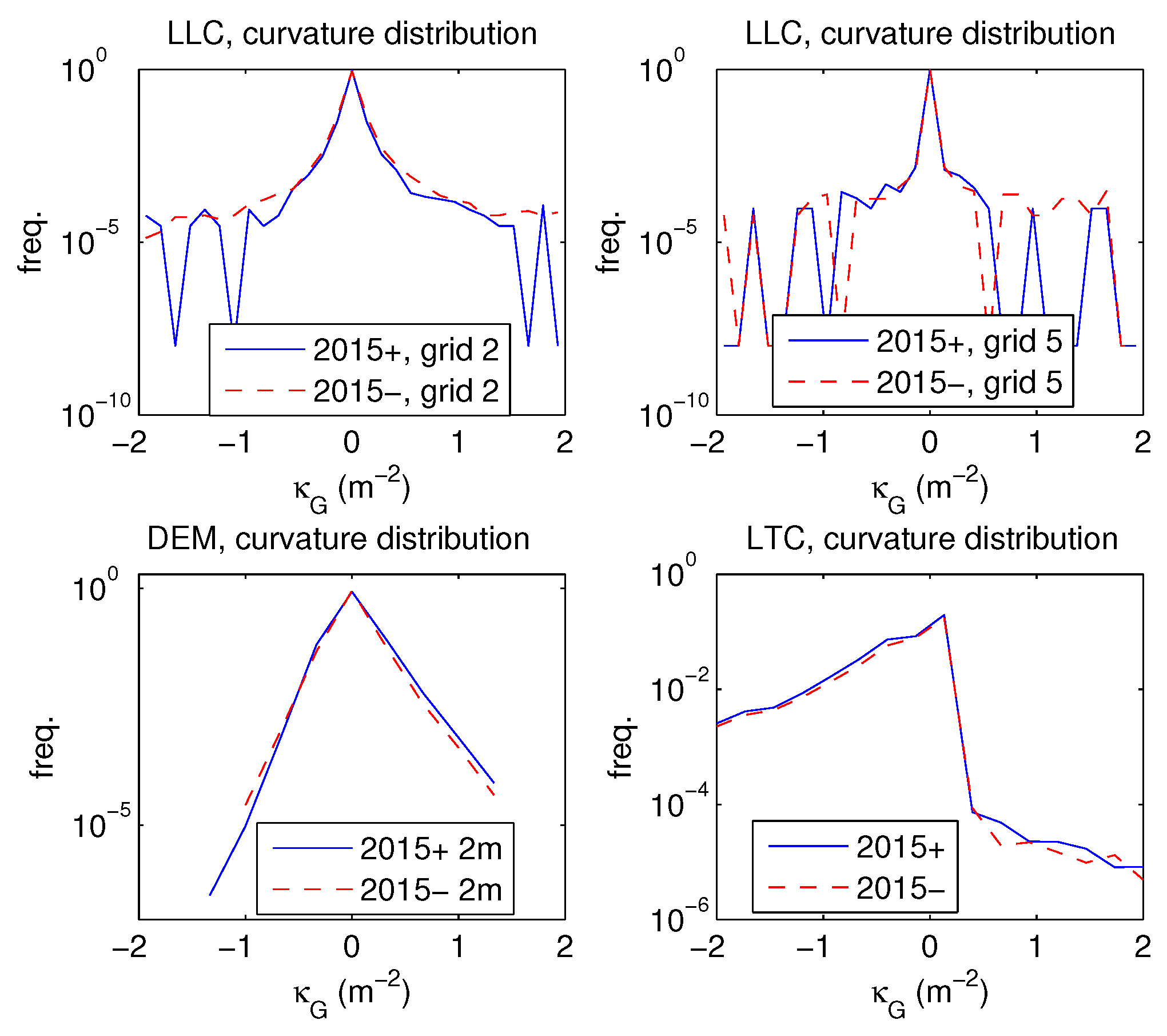
  • surface fitting methods: a parametric surface is fitted to data. Our local linear fit LLC falls on this category, yet does not necessarily require triangularization as a preliminary step.
  • total curvature methods: curvature approximant is derived as a function of location. Our local triangular curvature LTC is of this category of methods.
  • curve fitting methods.
LLC has a performance bottleneck in local linear fit procedure described in Section 2.5. This problem has been addressed recently in [30], where an algebraic-symbolic method is used to solve a set of total least squares problems with Gaussian error distribution in a parallelizable and efficient way. That method would require modification and experimentations with e.g., a gamma distributed error term due to asymmetric vegetation and canopy returns.
The vector voting method presented in [16] decreases noise and achieves good approximative surface normals for symmetrically noisy data sets of point clouds of technological targets. Our target cloud has asymmetrical noise (vegetation returns are always above the ground), and returns under the ground (e.g., reflection errors) are extremely rare. Usually vector voting methods are used in image processing. They are based on triangular neighborhood and any similarity measure between vertices, focusing signal to fewer points and making it sometimes easier to detect. Neighborhood voting possibilities are being discussed int Section 4.
General references of available curvature tensor approximation methods in case of triangulated surfaces are [31,32]. A derivation of Gaussian curvature κ G and mean curvature κ H is in [33]:
κ G = κ 1 κ 2
κ H = ( κ 1 + κ 2 ) / 2 ,
where κ l , l { 1 , 2 } are the two eigenvalues of the curvature tensor. Perhaps the best theoretical overview of general concepts involved in curvature approximation on discrete surfaces based on discrete differential geometry (DDG) is [34].
We experimented with methods which can produce both mean and Gaussian curvatures, giving access to curvature eigenvalues and eigenvectors. Our experiments failed since the mean curvature κ H seems to be very noise-sensitive to compute and would require a special noise filtering post-processing step. Difficulties in estimating the mean curvature from a noisy data have been widely noted, see e.g., [29].
In comparison to previous references, this paper is an independent study based on the following facts: point cloud density is low relative to the field objects of interest (stones), ratio of ground returns amongst the point cloud is high providing relatively even coverage of the ground, a direct approach without texture methods based on regular grids was preferred, individual stones are not tagged in the test data, and the methods are for a single focused application. Furthermore, we wanted to avoid complexities of segmentation-based filtering described in [35] and the method parameters had to be tunable by cross-validation approach.

2. Materials and Methods

Test data is presented in Section 2.2. It is available online, details are at the end of this paper.
Figure 1 presents the process flow of stone detection. Two data sources at left are introduced in Section 2.2, tested methods (DEC, LLC, LTC) are detailed in Section 2.5, Section 2.6 and Section 2.7. The vectorization of samples varies depending on the method in question, details can be found in Section 2.8. The solid angle filtering SAF of Section 2.4 is a necessary preprocessing step for LTC, but could be used also before LLC for computational gain.

2.1. Study Area

The study area is a rectangle of 1080 km 2 located in the Kemijärvi municipality, in Finnish Lapland, see Figure 2. The 675 sample polygons cover approx. 10.7 km 2 of the area. Mass-flow sediment fields such as the Kemijärvi field, have regional significance for aggregate production as there is an abundance of closely spaced mass-flow formations within a relatively short distance from the road network.

2.2. Materials

Table 1 gives a short summary of the data sets: the first set data2014 is rather small with positive samples occupied by large boulders. The second set data2015 has an imbalance of many positive samples with smaller stones vs. fewer negative samples. Data sets are depicted in Figure 2. The acquisition of data sets differ: the classification of data2014 was based on cumulated field photographs and the land survey annotations of the general topographic map (stone landmarks). There is no stone size distribution data available for data2014, though. The set data2015 was classified and the approximative stone size and coverage statistics recorded by a geology expert. The second data set seems to present more difficult classification task—the areas are more varied and stone size probably smaller than in the first set. The advantage of having two data sets of different origin is that the resilience and generality of the methods can be better asserted.
The data preprocessing consists of the following three steps:
  • All hummocky landforms (i.e., hills) with a convex topographic form were delineated from the ALS derived digital elevation model and its tilt derivative with an Object-Based Image Analysis algorithm developed in eCognition software, see [1]. This step produced data2014 and data2015 polygon sets ( see Table 1 and Figure 2).
  • A 10 m × 10 m space partitioning grid was used to cut both the point cloud (ALS) and DEM to polygon samples.
  • Point cloud was cut to 2 m height from initial approximate ground level. The mode of heights in 2 m × 2 m partitions was used as the ground level.
ALS LiDAR data was produced by National Land Survey (NLS) (NLS laser data: http://www.maanmittauslaitos.fi/en/maps-5) in fall 2012 with a Leica ALS50-II laser scanner (Leica Geosystems, St. Gallen, Switzerland), the flight altitude was 2000 m. Last-return data has approx. 0.09–0.1 m vertical ground resolution and average footprint of 0.6 m. ALS data has several additional information fields per cloud point, see e.g., [21]. We used only x-y-z components of the data. Approximately 25% of the data are canopy returns, the rest is ground returns. Reflection errors causing outlier points occur approximately once per 0 . 5 × 10 6 returns.
DEM data is 2 m regular grid data available from NLS. It is nationwide data aimed for general purposes (geoengineering, construction industry). Its vertical accuracy is 0.3–1.0 m std. Both ALS and DEM data were cut to polygon samples by using 10 m × 10 m space partitioning slots. See two example polygon shapes in Figure 3. The further processing focused only to the point cloud limited by each polygon sample.
Stones are bare and the vegetation is thin due to high Northern latitudes.The point cloud on this site has approx. 25 % returns to forest canopy and approx. 75 % ground returns, so the ground signal is rather strong. The reflection errors were extremely rare, approx. 1 per 10 6 returns. Together the sample sets represent rather well the Kemijärvi study area.

2.3. Materials online

Sample data sets including some polygon point clouds, DEM data of two map pages, sample vectors, some field images, SAF algorithm document, a short description of the data set and the problem are available at: http://users.utu.fi/ptneva/ALS/.

2.4. Solid Angle Filtering (SAF)

The proposed solid angle filtering is a novel method to produce an alternative TIN DEM sensitive to stones and boulders on the ground. Filtering starts by forming an initial TIN either from a full point cloud or after an industry standard preliminary canopy and tree point elimination. The cut was made 2 meters above the local mode of the point cloud height. The 2D projection of TIN satisfies Delaunay condition at all times during the iterative process of point elimination. The prominent ’pikes’ in the intermediate TIN are removed in random order while the Delaunay triangulation is updated correspondingly. The implementation requires a dynamical Delaunay algorithm, which facilitates incremental removal of points. We used an industry standard approach described in [36] with O ( k ) computational complexity per removed point, where k stands for the average number of nearest neighbors of a point.
A second iterative phase removes ‘pits’ in a similar fashion. The prominence of pikes and pits is measured by solid angle Ω k , which is the spatial angle of the surrounding ground when viewed from a TIN vertex point p k . Appendix A provides the technical definition of computing Ω k .
Each state of TIN is achieved by dropping one point which fails the following inequality:
Ω m i n Ω k Ω m a x ,
where solid angle limits Ω m i n = 1 . 80 sr (steradians) and Ω m a x = 12 . 35 sr correspond to solid angles of two spherical cones with opening angles 89 and 330 , respectively. The choice affects the prediction performance: if both limits are close to a planar situation of Ω 2 π , there is a loss of points. If there are no limitations ( Ω m i n 0 , Ω m a x = 4 π ), data is dominated by the noise from canopy and tree trunks. The solid angle limits were defined by maximizing the Kolmogorov-Smirnov (K-S) test [37] difference using 95 % confidence limit. Figure 4 depicts the difference between solid angle distributions at positive and negative sample sets at the choice we made. A pike at approx. 2.5 sr indicates stones.
The resulting ground surface triangularization (see lower left part of Figure 2) resembles the end product of the 3D alpha shape algorithms [38], when alpha shape radius is chosen suitably. It produces an alternative TIN model which hopefully contains a signal needed in stone detection. In this paper this method is used as a preprocessing step for LTC method (see Section 2.6) and for LLC method (see Section 2.5, and Figure 1).

2.5. Curvature Estimation Based on Local Linear Fit (LLC)

LLC method is based on a curvature approximation method described in [33]. The method requires surface normals to be available at the triangle vertices. LLC provides these normals by a local linear fit to the point cloud at a regular horizontal grid. Since the resulting curvature function is not continuous at the border of the triangles, a voting procedure is needed to choose a suitable value for each grid point.
Finding the local planes is a similar task to finding the moving total least squares (MTLS) model in [39]. The differences are the following:
  • a space partitioning approach is used instead of a radial kernel function to select the participant points. This is because ground surface can be conveniently space partitioned horizontally unlike in [39], where the point cloud can have all kinds of surface orientations.
  • the point set is not from constructed environment. Canopy returns create a 3D point cloud, thus the loss function cannot be symmetrical, but must penalize points below the approximate local ground plane.
The LLC process has 6 steps, which are expounded in Appendix B. Step 1 is cutting the foliage dominated part of the point cloud, step 2 approximates ground with local linear planes at regular grid points. Step 3 spans the grid with triangles avoiding spots with missing data. Step 4 defines the curvature within each triangle. Step 5 combines the curvature values of the neighboring triangles to each grid point. Step 6 is about forming a histogram over the whole grid of the sample polygon.
LLC is a multi-scale method like [28]. Steps 1 through 6 are repeated with differing grid lengths δ j , j [ 1 , 6 ] of the grid, see Table 2. There is a potential danger for overfitting, so the qualities of grid sizes are discussed here from that point of view.
The smallest grid size δ 1 = 1 . 25 m has approx. 85 % of the grid slots with only 1 to 3 points as shown in the left part of Figure 5 and so it represents a practical low limit of the local planar fit. A practical upper limit is δ 6 = 6 m because only the largest boulders get registered on this scale. Such large boulders are few, as shown in the right part of Figure 5.

2.6. Local Curvature Based on Ground Triangularization (LTC)

The input is a triangulated surface model generated by SAF method described in Section 2.4 and Figure 1. LTC produces the curvature estimates directly to the vertex points, so local linearization step 3 of the LLC method of Section 2.5 is not needed. Vectorization (step 4 of LLC) has to be done, but only once, since there are no grids nor multi-grids in this method. The idea is to calculate the value κ k of a Gaussian curvature operator at each ground point p k based on the Gauss-Bonnett theorem as described in [31].
The right side of the Figure A1 depicts a point p k and its neighboring points p i and p j . The neighboring triangles T k of a vertex point k define a so-called spherical excess, which is the difference between the sum of triangular surface angles β i k j and the full planar angle 2 π . Now, one can write an estimator for the Gaussian curvature κ k at point p k based solely on local triangularization formed by the Delaunay process:
β i k j = acos ( p i p k , p j p k )
A k = t T k A t / 3
κ k 2 π ( i , k , j ) T k β i k j / A k ,
where β i k j is the angle at vertex k in a surface triangle t = ( i , k , j ) T k , acos ( . , . ) is the angle between two vectors defined in Equation (A1) in Appendix A, and A k is a characteristic surface area associated with the vertex k. The characteristic area has been defined approximately by taking one third of the area A t of each adjoining triangle t. There are locally more stable but also more complicated ways to calculate A k , see e.g., [31,32]. The choice made in Equation (4) causes noise because the area is approximate but seems to allow effective histogram vectors.

2.7. Curvature Based on Filtering DEM by a Modified Discrete Laplace Operator (DEC)

The third method is traditional, fast and easy to implement in the GIS framework and thus provides a convenient baseline for the previous two methods. Local height difference is converted to local curvature approximant. Curvature histograms are then vectorized as in previous methods.
DEM data with a regular grid with the grid size δ = 2 . 0 m was utilized. Data is publicly available over most of Finland. The discrete 2D Laplace operator with radius r h o r i z = 2 . 0 m is well suited for detecting bumpy features like stones at the grid detection limit. It simply returns the difference between the average height of 4 surrounding grid points and the height of the center point. A modified Laplacian filter with r h o r i z = 4 . 0 m (length of two grid squares) was used to estimate the local height difference on the larger scale, see Figure 6. A postprocessing transformation by Equations (7) and (8) was applied to produce correspondence to Gaussian geometric curvature κ k at point k. A geometric justification for the transformation is depicted in Figure 6. A stone is assumed to be a perfect spherical gap with perfect horizontal surrounding plane. The mean curvature κ H can be approximated from the observed local height difference of Equation (6) by using the geometric relation Equation (7), see Figure 6. z ¯ ( r h o r i z ) is the average height at the perimeter of horizontal radius r. The local height difference Z ¯ is the key signal produced by Laplacian filter. Gaussian curvature is approximately the square of the mean curvature, when perfect sphericality is assumed, see Equation (8). The sign of the Gaussian curvature approximant κ G k at point c k can be decided on the sign of the height difference Z ¯ at vertex k. The index k of the vertex point p k is omitted for brevity. Equation (7) comes from rectangular triangle in Figure 6.
Z ¯ = z z ¯ ( r ) local height difference
1 / κ H 2 r h o r i z 2 + ( 1 / κ H Z ¯ ) 2 approximate mean curvature condition
κ H 2 Z ¯ / ( Z ¯ 2 r h o r i z 2 ) mean curvature solved from Equation ( 7 )
κ G sign ( Z ¯ ) κ H 2 approximate Gaussian curvature
Figure 6 shows grid squares of size 2 m × 2 m . Points A are used to calculate the average height z ¯ ( 2 . 0 m ) and points B the average height z ¯ ( 4 . 0 m ) .
Many sample polygons are relatively small. The above described difference operator produces numerical boundary disturbance, see Figure 3. This can be countered by limiting the perimeter average z ¯ ( r ) only to the part inside the polygon, and then removing the boundary pixels from the histogram summation.
The next step is to build the sample histograms as with other methods. Histogram vectors from two filters are concatenated to produce a sample vector of a polygon. The details of forming the histogram are given in Section 2.8.

2.8. Vectorization

All three methods produce histograms of Gaussian curvature κ G = ± 1 / r 2 , where r is the local characteristic curvature radius and the curvature sign has been chosen in Equation (8) so that potential stone tops have negative curvature and “pit bottoms” have positive curvature. An ideally planar spot k has curvature radius r k and curvature κ G 0 . Recall that minimum detectable stone radius is approx. r m i n = 0 . 6 . . . 1 . 2 m, which leads to a Gaussian curvature interval of κ G = [ 1 . 8 , 1 . 8 ] m 2 . This range was spanned by histogram bins. LLC and DEC are rather insensitive to bin choice, so a common ad hoc choice was made for these methods, see Table 3. The LTC method proved sensitive to bin choices, so the values were derived using a subset of 10 positive and 10 negative samples in leave-pair-out cross-validation. This set was excluded from later performance measurements.
The histogram creates a vector representation x i , i = 1 . . n for all sample polygons i. The LTC method produces one histogram vector, the DEC method produces two vectors (for r = 2 and r = 4 m) and LLC produces 6 vectors (for 6 different grids), which are then concatenated to form the final sample vector x i .
Figure 7 provides a summary of average curvature distributions produced by each of the three methods. The planar situation with κ G 0 is the most common. Occurrences with characteristic radius r < 1 m are very rare. Useful information is contained within the range κ G [ 1 , 1 ] m 2 . With LLC method, grid size δ = 2 m is able to detect greater curvatures and grid size δ = 5 m is the last useful grid size. DEM is remarkably similar to 2 m LLC grid, which was to be expected.
Negative samples (dashed lines) have about the same amount of exactly planar samples, but are a little bit more slightly curved ( | κ G | 0 . 4 m 2 ) samples. This probably results from the basic ground curvature distribution. If the presented three methods were to be adapted elsewhere, the changing background curvature spectrum may result in changes in the prediction performance.
The LTC method is able to detect the negative curvature around the stone causing the curvature distribution to be asymmetric. Unfortunately, this method is also very noise-sensitive reducing its performance.
Each method requires more testing and especially test data with known stone properties (relative coverage of the surface, radius and height distribution, individually located and labeled stones).

2.9. Logistic Regression

The label vector y i { 1 , 1 } , i D = 1 . . . n was acquired by field campaign done by a geology expert. D is the index set of the full sample set, size n = | D | varies depending e.g., on the different sensitivity to sparse point cloud of each method. The sample vectors x i R d are produced by histogram vectorization described in Section 2.8. Dimensionality d varies depending on the method. We use the affine form z i = ( 1 , x i ) to shorten the following treatise. Vectors { z i } i D are also standardized before solving the regression problem.
This is a qualitative response problem, so logistic regression was chosen to predict a label y ^ from a given sample vector x . The prediction coefficient β R d + 1 is tuned by usual maximum likelihood approach to optimal value β D * using a sample set { ( z i , y i ) } i D , D D where D is the training set used:
f ( z i , β ) = P r ( y i = 1 | z i ) = 1 + exp β · z i 1 y ^ ( D ) ( z ) = 1 when f ( z , β D * ) 1 / 2 1 otherwise
The area under curve (AUC) performance measure is natural in this application area, where cost functions do exist but are not exactly known. The sample set data2014 is rather small and the sample set data2015 has imbalanced samples of positive and negative cases and the n-fold cross-validation may produce too optimistic estimates, as mentioned in [40]. It is recommended in [40] in this case:
  • to perform a leave-pair-out (L2O) test over all possible positive-negative label pairs P, and
  • to measure L2O area under curve A U C by using the Heaviside function H ( . ) for summation.
P = { ( i , j ) | y i = 1 , y j = 1 , i , j D } all possible ( + , ) pairs A U C = ( i , j ) P H ( y ^ i j ( z i ) y ^ i j ( z j ) ) / | P | leave - pair - out AUC y ^ i j ( z ) = y ^ ( D { i , j } ) ( z ) prediction without a pair i , j based on z H ( Δ y ^ ) = 1 + sign ( Δ y ^ ) / 2 Heaviside over the prediction difference

2.10. Method Parameters and Design Choices

Some parameters were optimized by nested cross-validation or K-S test and thus settled. Some parameters are ad-hoc built-in parameters, values of which are chosen mostly during the coding process. These should be taken into consideration if the methods are utilized under slightly different conditions. A list of the open parameters, their potential range and some of the discrete design choices available, follows. Table 4 is a summary of the treatise.
LLC: There are 11 non-zero shape parameters of the planar distance weight function g ( . ) presented in [11]. The validation of the choices made will be a separate publication. There are some minor design choices, an example is Equation (B2): one can use either median or mean rule in composing curvature from surrounding triangle vertices, and results do not change noticeably. Median rule was used to reduce occasional outliers. Another example is the 6 grid sizes in Table 2. The number of possible subsets of grids to be used equals 2 6 1 = 63 .
LTC: There is a design choice of using the local surface area A t / 3 in Equation (4) or a more complex definition given in [32]. This is listed as one binary choice in Table 4.
DEC: There is a binary choice of either choosing Laplacian filter signal Z ¯ or the Gaussian approximant κ k of Equation (8) based on the signal Z ¯ .

2.11. General Wall-to-Wall Prediction

Methods presented in Section 2.4, Section 2.5, Section 2.6, Section 2.7, Section 2.8 and Section 2.9 were applied only to given polygon areas, since teaching is possible only where the response value is known. But after the parameters of predictor have been settled, the area to be inspected can be a generic one. As a demonstration and speed test, we applied methods to a 1080 km 2 area divided to 20 m × 20 m pixels with approx. 320 points from a point cloud of density ρ = 0 . 8 m 2 . Pixels have 6 m overlapping margins to increase the sample area to 32 m × 32 m (approx. 820 points) to avoid partially populated histograms, which would not be recognized correctly by the classifier. See Figure 8 for the DEC method wall-to-wall result.

3. Results

Binary classification of stoniness was done by logarithmic regression over curvature histogram vectors cumulated over each sample polygon area. Three methods were used; they differ on how the curvature approximants were produced(Table 5):
  • Local linear fitting (LLC) divides the polygon into 6 different grids. Each grid square is fit by a plane approximating the local ground height of the center of the plane and the plane orientation. Curvatures are computed from these center points and their orientation normals.
  • Curvature from DEM (DEC) uses traditional DEM data. Curvatures are approximated by the observed local height difference delivered by a modified discrete Laplace operator.
  • Curvature by local triangulation (LTC) has a TIN computed by SAF method of Section 2.4. The curvature is then computed triangle by triangle as in LLC.
Area under curve AUC [41] was measured using both data sets and all three methods, see Section 2.9. The AUC measure describes the discriminative power of a predictor over various possible cutoff point choices. A proper cutoff depends on the costs involved and is not known at the moment, justifying the accommodation of AUC. Leave-pair-out variant of AUC was used, see considerations for this choice in Section 2.9.
LLC proved best for data2015. This data set is large and perhaps more representative of the locality, and the performance A U C = 0 . 77 can be considered adequate for practical application such as pre-selecting possible gravel deposit sites for infrastructure construction. Its performance is also on par with many hard natural resource prediction tasks based on open data, see e.g., [2].
Data set data2014 is somewhat exceptional, since it contains larger boulders and seems to be an easy prediction task for wide array of methods. Both DEC and LLC performed well. The same holds to several other tested methods which have not been included to this report, e.g., neighborhood voting based on solid angle values.
DEC performance is mediocre with data2015 set because the average stone size depicted in Figure 5 right side is actually below the theoretical detection limit of a regular 2 m grid. Established DEM computation routines are a trade-off of many general-purpose goals and some of the stone signal seems to be lost in the case of the data2015 set.
LLC, eventhough it was cross-validated with data2014, performed adequately here. There were high hopes about local curvature based on triangularization (LTC), but it performed the worst. This is because LTC computes the curvature directly from a TIN, and the process produces a lot of noise. LTC has been included in this report mainly because the method is fast to compute and there seems to be potential to reduce noise in the future by neighborhood voting methods.
The processing speed (see Table 6) has a linear dependence with the area analyzed. This is because the analysis is done by space partitions of constant point cloud sample size n. All the steps have a linear O ( n ) time complexity except the Delaunay triangulation in SAF. The point removal phase in SAF is of O ( k n ) complexity, where k 5 . . . 20 is the amount of nearest neighboring points. The experiments were run on a desktop computer with Intel Core i5-3470 CPU (3.20 GHz) running Ubuntu Linux 14.10. LLC implementation requires several intermediary file operations, which makes it slow. All implementations are experimental prototypes and many speed improvements are still possible.

4. Discussion

A traditional approach for terrain micro-topography classification is to use DEM model as a basis for a wide array of texture methods. The low end has a simple texture feature computation followed by segmentation tuned manually by an expert. The high end has several texture features extracted, and preferably at least two DEM models of different grid size as a basis for analysis.
This paper presents a way to use the existing ALS LiDAR material to construct an alternative task-specific terrain surface representation which hopefully contains more information e.g., concerning the presence of stones. All methods presented are conceptually simple, although documenting and coding LLC and LTC brings up a multitude of details and ad hoc choices, see e.g., the number of method parameters in Table 4. Each method has potential for further improvement by a more thorough parameter tuning. SAF and LLC have enough method parameters that tuning by new field campaign data at more southern boreal forests could succeed. More southern boreal forest provides a challenge since the ratio of the ground returns is only 30%–60% instead of 70% at our Northern test site.
LLC and DEC perform well enough to be practically usable. The direct utilization of ALS data seems to work on this site.
Because LTC is based on a TIN model, there is available additional geometrical information like mean curvature, curvature eigenvalues and eigenvectors etc. for more complex micro-topographic features. If it is possible to reduce the noise and keep the computation costs at the current low level, a combination of these features could be a basis for fruitful multi-layer texture analysis.
Many terrain micro-topography classification tasks e.g., registering post-glacial landslides, karst depresssion detection and fault lines detection e.g., can be done with DEM and by texture methods, but there may be a need to add stoniness or curvature related features to improve the classification. The current data sets do not provide accurate quantitative information about stoniness for regression methods. The wall-to-wall stoniness result with 20 m × 20 m pixels produced by current binary classification (see Figure 8) can be utilized as an additional feature in other prediction problems in the future. The wall-to-wall pixel size must be increased when the ground return ratio decreases in the southern dense forests.
Three individual methods or a combination of them can be modified to produce estimates of the relative stone coverage and stone size distribution. This step can be taken only if data sets come available with individual stones and their properties tagged out. Furthermore, more sophisticated probabilistic and minimum description length (MDL) based methods would then be possible. The stone coverage and size distribution information in Figure 5 is approximative only, so current data sets cannot be used for development of quantitative stoniness models.
It is hard to estimate how far to southern forests the three methods can be extended. The ground return density varies with boreal forests, and detection results from spatially rather sparse accessible spots should be somehow extended to nearby areas using other available public data and Machine Learning methods. This line of research requires specific field test sets, though.
There are several other micro-topological problems, e.g., classifying and detecting undergrowth, marshland types, military structures, unauthorized inhabitation and geomorphology e.g., frost phenomena. Some of these require comparison of two snapshots from ultra-light vehicle (UAV) scans, and e.g., a combination of SAF and MDL might perform well in this scenario. We believe SAF has wide adaptivity to several purposes by tuning its 2 parameters (minimum and maximum spatial angle allowed) and MDL can be built to detect a specific shape (a hemisphere in cases of stones, a box, a prism or a cylinder in case of other applications). As mentioned before, MDL would require denser point clouds with ρ 1 . 6 . . . 3 . 2 m 2 .

5. Conclusions and Future Research

Results in Section 3 show that LLC performs better than DEC but is numerically much more expensive. LLC seems to be robust and useful when the computation costs can be amortized over several subsequential analyses. LTC performed worst but there is room for improvement as discussed in Section 4. Both LLC and DEC are ready to be applied to industrial purposes after prototyping implementations are upgraded to production code.
Current results are bound to stoniness of mass-flow deposits what comes to teaching data, but each method should work in generic stoniness detection, if such a need arises and general teaching data sets become available.
Using direct ALS information either as an alternative data source or supplementary one may help solving a variety of micro-topography detection problems better in the future. The research efforts will be focused on the following topics:
  • Extending the analysis to more dense forests, where stoniness detection occurs only at benevolent cicumstances (forest openings, sparse canopy, hilltops). In this environment the acquired stoniness signal has to be combined to a wide array of open data features to extend prediction to unobservable areas. The corresponding field campaigns will be more elaborate.
  • Taking into account the stone coverage and size distribution. It is likely that a multi-grid method like LLC might perform well in this prediction task (given suitable teaching data), whereas DEC may be restricted by the general purpose nature of DEM and its modest grid size.
  • Topography and vegetation classification of marshlands. Marshlands have similar high ground return ratio as the current case site. SAF can be tuned by cross-validation to produce a tailored TIN and an improved LTC method with added curvature properties (mean curvature, curvature eigenvectors) could detect various micro-topographic marshland features. It is our assumption that the histogram approach would work also with marshland classification, given a suitable teaching polygon quality produced in field campaigns.
  • Using min-cut based segmentation of k-NNG graph of ALS data as described in [15] instead of simple Delaunay triangulation. One has to modify the algorithm to include neighborhood voting to reduce noise. This could be a fruitful approach, since it could suit to 3D analysis of forest tree species, providing more motivation for the implementation.
  • Utilizing all relevant LiDAR attribute fields, like return intensity, return number, the scan angle etc. (see [21]).

Acknowledgments

Department of Information Technology of University of Turku covered the travel and publication costs. English language was revised by Kent Middleton.

Author Contributions

Maarit Middleton designed and conceived the sample polygon sets; Raimo Sutinen conceived the research problem; Paavo Nevalainen designed the methods and analyzed the data; Paavo Nevalainen wrote the paper; Jukka Heikkonen contributed to the paper; Tapio Pahikkala contributed to the performance analysis.

Conflicts of Interest

The authors declare no conflict of interest.

Abbreviations

The following abbreviations are used in this manuscript:
ALSAerial laser scan
AUCarea under curve
DDGDiscrete differential geometry
DECCurvature based on DEM
DEMDigital elevation model
DTMDigital terrain model
GISGeographic information system
k-NNGk-nearest neihgbors graph
K-SKolmorogov-Smirnov test
L2OLeave-pair-out
LiDARLight detection and ranging
LLCcurvature based on local linear fit
LTClocal curvature based on ground triangulation
MDLMinimum description length principle
MTLSMoving total least squares
NLSNational Land Survey of Finland
PCAprincipal components analysis
SAFSolid angle filtering
TINtriangulated irregular network
UAVUltra-light vehicle

Appendix A

The computation of a solid angle Ω k takes place at the approximity of a point p k , namely at the set of the adjoining triangles T k , see detail A) of Figure A1. Detail B) presents a tetrahedron defined by points p k , p i , p j , p l , where p i , p j T k p k are from the outskirt of the triangle set T k and p l is an arbitrary point directly below point p k . There are several ways to implement the solid angle calculation, a formula based on a classical l’Huillier’s theorem [42] is presented here:
acos ( a , b ) = cos 1 ( a 0 · b 0 ) angle between two vectors x 0 : = x / x 2 vector normalization α i = acos ( p l p k , p j p k ) compartment angles i , j , k α j = acos ( p i p k , p l p k ) α l = acos ( p j p k , p i p k ) α 0 = α i + α j + α l basic product term
ω i l j = 4 tan 1 tan α 0 4 Π ν { i , j , l } tan α 0 2 α ν 4 compartment angle
Ω k = i l j T k ω i l j solid angle at point p k
Figure A1. Solid angle filtering. (A) The set of adjoining triangles T k of a point p k seen from above; (B) A compartment i j l of the vertex point p k presented in detail. A solid angle Ω k is a sum of compartment angles ω i l j of Equation (A2). Point p l is an arbitrary point directly below the vertex point p k .
Remotesensing 08 00720 g009
Equation (A2) approaches so called Heron’s planar trigonometric formula [42] when angles α i , . . . approach zero. The practical implementation requires a combination of space partitioning to a manageable point cloud patches of approx. 700...2000 points and a 2D Delaunay triangulation with an efficient point removal method. We use a batch version (python scipy.spatial.delaunay) with our own industry standard routine for deletion. This combination is simple to implement and excels in practise as [36] mentions, even though there exists faster incremental deletion arrangements with 2..3 times slower construction phase.

Appendix B

Step 1: Data can be preprocessed in three different ways before the LLC step. Alternatives are listed here in the order of increasing computational efficiency and decreasing amount of points:
(a)
raw 3D ALS data
(b)
same as (a) with tree and foliage returns cut from approx. 2 m height from approximative ground level
(c)
TIN model produced e.g., by solid angle filtering of Section 2.4
The local linear fitting step 2 finds similar ground model per each alternative, only the speed of convergence varies. All three alternatives seem to result in about the same quality when measured by predictor performance.
Step 2: The fitting of the plane resembles a normal regression problem with an ad hoc nonlinear loss function, which penalizes residuals below the plane to force the ground fit. By applying the fitting process to planes of varying sizes one gets an assembly of plane orientations and plane centers. The neighboring planes can then be used to approximate local curvature. Since sample density is low, some of the plane fits cannot be performed. Therefore, it is numerically more resilient to use triangulation over neighboring planes and define curvature over each triangle using formulation developed in [33]. Another approach would be to produce a triangular mesh and estimate curvature based on it, as in [31,32]. There is a large filtering effect in this approach, since vertex normals depend on surrounding vertices. Local linear fit seemed to pick up the stoniness signal better, especially since we used multi-scale grids.
The grid division has been depicted in Figure B1. At each grid slot, one has to find the best fitting plane P ( p , n ) , where p R 3 is the center point of the plane P and n its normal. The initial state for the plane is: P 0 = P ( lowest point of local sample , ( 0 , 0 , 1 ) T ) δ .
The plane P represents a good local ground linearization provided that the weight function g ( l ) of the orthogonal distance l penalizes heavily points below the approximated ground level. The details of weight function have been published in [11]. The practical considerations in selecting the weight function shape are at rapid and guaranteed convergence, whereas the influence to prediction performance comes from the actual ground returns and their geometry.
Figure B1. Left: An individual local plane P ( p k , n k ) at grid point c k and its parameters (local plane center point p k and normal n k ). A triangulation T of the grid avoids squares with incomplete data. A local cloud point set Q c k and neighboring triangles T k T of a grid slot c k are also depicted. Center: a stone revealed by two adjacent tilted planes. This stone provides a signal with the grid size δ = 2 m. Note the amount of missing planes due to a lack of cloud points. Right: The grid of size δ = 4 m at the same spot. The stone does not appear, local variation has disappeared but the grid is almost full approximating the sample polygon shape.
Remotesensing 08 00720 g010
The optimal fit at each grid slot concerns now coordinate components w T = ( p z , n x , n y ) of p and n . The local plane P is found by a numerical minimization:
w * = arg min w q j Q c g [ ( q j p ) · n ]
Step 3: Triangulation is based on the grid centers, where the surface normal is known. Because of relatively low point density, some grid locations are bound to have no points and thus have to be omitted from triangulation, see Figure B1. The triangularization T outlined in Figure B1 is generated randomly, see Figure B1. The end result dictates the adjoining triangle sets T k T of each grid point k. The size | T k | of the adjoining triangle sets varies depending on how dense or sparse point cloud is nearby point k: 1 | T k | 8 .
Step 4: The curvature is approximated on each vertex of each triangle as in [33]. There are several other similar formulations e.g., using rectangular grids, but those are not so suitable in the presence of sparse and missing cloud points. The end result is set of candidate curvatures κ t k , t T k per each grid point p k .
Step 5: Now the task is to combine the final curvature approximant at a grid point p k by taking a median of values available at the adjoining vertices of all surrounding triangles:
κ ( p k ) = median t T k κ t k
Step 6: We used the normalized histograms of h = hist k K κ ( p k ) , where K is the set of grid centers and histogram operator hist(.) and its properties are documented in Section 2.8.

References

  1. Middleton, M.; Nevalainen, P.; Schnur, P.; Hyvnen, T.; Sutinen, R. Pattern recognition of mass-flow deposits from airborne LiDAR. In Proceedings of the 36th EARSeL Symposium, Bonn, Germany, 20–24 June 2016.
  2. Pohjankukka, J.; Nevalainen, P.; Pahikkala, T.; Hyvönen, E.; Middleton, M.; Hänninen, P.; Ala-Ilomäki, J.; Heikkonen, J. Predicting water permeability of the soil based on open data. In Proceedings of the 10th Artificial Intelligence Applications and Innovations (AIAI 2014), Rhodes, Greece, 19–21 September 2014.
  3. Palmu, J.P.; Ojala, A.; Ruskeeniemi, T.; Sutinen, R.; Mattila, J. LiDAR DEM detection and classification of postglacial faults and seismically-induced. GFF 2015, 137, 344–352. [Google Scholar] [CrossRef]
  4. Johnson, M.D.; Fredin, O.; Ojala, A.; Peterson, G. Unraveling Scandinavian geomorphology: The LiDAR revolution. GFF 2015, 137, 245–251. [Google Scholar] [CrossRef]
  5. Sutinen, R.; Middleton, M.; Liwata, P.; Piekari, M.; Hyvönen, E. Sediment anisotropy coincides with moraine ridge trend in south-central Finnish Lapland. Boreas 2009, 38, 638–646. [Google Scholar] [CrossRef]
  6. Sutinen, R.; Hyvönen, E.; Kukkonen, I. LiDAR detection of paleolandslides in the vicinity of the Suasselk posglacial fault, Finnish Lapland. Int. J. Appl. Earth Obs. Geoinf. A 2014, 27, 91–99. [Google Scholar] [CrossRef]
  7. Alho, P.; Vaaja, M.; Kukko, A.; Kasvi, E.; Kurkela, M.; Hyyppä, J.; Hyyppä, H.; Kaartinen, H. Mobile laser scanning in fluvial geomorphology: mapping and change detection of point bars. Z. Geomorphol. Suppl. 2011, 55, 31–50. [Google Scholar] [CrossRef]
  8. Sutinen, R.; Hyvönen, E.; Middleton, M.; Ruskeeniemi, T. Airborne LiDAR detection of postglacial faults and Pulju moraine in Palojärvi, Finnish Lapland. Glob. Planet. Chang. 2014, 115, 24–32. [Google Scholar] [CrossRef]
  9. Gallay, M. Geomorphological Techniques, 1st ed.; Chapter Section 2.1.4: Direct Acquisition of Data: Airborne Laser Scanning; British Society for Geomorphology: London, UK, 2012. [Google Scholar]
  10. Li, Z.; Zhu, C.; Gold, C. Digital Terrain Modeling; CRC Press: Roca Baton, FL, USA, 2004. [Google Scholar]
  11. Nevalainen, P.; Kaate, I.; Pahikkala, T.; Sutinen, R.; Middleton, M.; Heikkonen, J. Detecting stony areas based on ground surface curvature distribution. In Proceedings of the 5th International Conference Image Processing, Theory, Tools and Applications IPTA2015, Orléans, France, 10–13 November 2015.
  12. Waldhauser, C.; Hochreiter, R.; Otepka, J.; Pfeifer, N.; Ghuffar, S.; Korzeniowska, K.; Wagner, G. Automated Classification of Airborne Laser Scanning Point Clouds. Solv. Comput. Expens. Eng. Probl. Proc. Math. Stat. 2014, 97, 269–292. [Google Scholar]
  13. Meng, X.; Currit, N.; Zhao, K. Ground Filtering Algorithms for Airborne LiDAR Data: A Review of Critical Issues. Remote Sens. 2010, 2, 833–860. [Google Scholar] [CrossRef]
  14. Haugerud, R.; Harding, D. Some algorithms for virtual deforestation (VDF) of LiDAR topographic survey data. Int. Arch. Photogramm. Remote Sens. 2001, 34, 219–226. [Google Scholar]
  15. Golovinskiy, A.; Funkhouser, T. Min-Cut Based Segmentation of Point Clouds. In Proceedings of the IEEE Workshop on Search in 3D and Video (S3DV) at ICCV, Kyoto, Japan, 27 September–4 October 2009.
  16. Page, D.L.; Sun, Y.; Koschan, A.F.; Paik, J.; Abidi, M.A. Normal Vector Voting: Crease Detection and Curvature Estimation on Large, Noisy Meshes. Graph. Model. 2002, 64, 199–229. [Google Scholar] [CrossRef]
  17. Johnson, K.M.; Ouimet, W.B. Rediscovering the lost archaeological landscape of southern New. J. Archaeol. Sci. 2014, 43, 9–20. [Google Scholar] [CrossRef]
  18. Vosselman, G.; Zhou, L. Detection of curbstones in airborne laser scanning data. ISPRS, 2009; pp. 111–116. [Google Scholar]
  19. Brubaker, K.M.; Myers, W.L.; Drohan, P.J.; Miller, D.A.; Boyer, E.W. The Use of LiDAR Terrain Data in Characterizing Surface Roughness and Microtopography. Appl. Environ. Soil Sci. 2013, 2013, 1–13. [Google Scholar] [CrossRef]
  20. Hengl, T.; Reuter, H. (Eds.) Geomorphometry: Concepts, Software, Applications; Elsevier: Amsterdam, The Netherland, 2008; Volume 33, p. 772.
  21. ASPRS. LAS Specification Version 1.4-R13; Technical Report; The American Society for Photogrammetry & Remote Sensing( ASPRS): Bethesda, ML, USA, 2013. [Google Scholar]
  22. Weishampel, J.F.; Hightower, J.N.; Chase, A.F.; Chase, D.Z.; Patrick, R.A. Detection and morphologic analysis of potential below-canopy cave openings in the karst landscape around the Maya polity of Caracol using airborne LiDAR. J. Cave Karst Stud. 2011, 73, 187–196. [Google Scholar] [CrossRef]
  23. Telbisz, T.; Látos, T.; Deák, M.; Székely, B.; Koma, Z.; Standovár, T. The advantage of lidar digital terrain models in doline morphometry copared to topogrpahic map based datasets—Aggtelek karst (Hungary) as an example. Acta Carsol. 2016, 45, 5–18. [Google Scholar] [CrossRef]
  24. de Carvalho Júnior, O.A.; Guimaraes, R.F.; Montgomery, D.R.; Gillespie, A.R.; Gomes, R.A.T.; de Souza Martins, É.; Silva, N.C. Karst Depression Detection Using ASTER, ALOS/PRISM and SRTM-Derived Digital Elevation Models in the BambuiGroup, Brazil. Remote Sens. 2014, 6, 330–351. [Google Scholar] [CrossRef]
  25. Kobal, M.; Bertoncelj, I.; Pirotti, F.; Kutnar, L. LiDAR processing for defining sinkhole characteristics under dense forest cover: A case study in the Dinaric mountains. Int. Arch. Photogramm. Remote Sens. Spat. Inf. Sci. 2014, XL-7, 113–118. [Google Scholar] [CrossRef]
  26. Hulík, R.; Španěl, M.; Materna, Z.; Smrž, P. Continuous Plane Detection in Point-cloud Data Based on 3D Hough Transform. J. Vis. Commun. Image Represent. 2013, 25, 86–97. [Google Scholar] [CrossRef]
  27. Yang, M.Y.; Förstner, W. Plane Detection in Point Cloud Data; Technical Report TR-IGG-P-2010-01; University of Bonn: Bonn, Germany, 2010. [Google Scholar]
  28. Evans, J.S.; Hudak, A.T. A multiscale curvature algorithm for classifying discrete return lidar in forested environments. IEEE Trans. Geosci. Remote Sens. 2007, 45, 1029–1038. [Google Scholar] [CrossRef]
  29. Pauly, M.; Keiser, R.; Gross, M.; Zrich, E. Multi-scale Feature Extraction on Point-sampled Surfaces. Comput. Graph. Forum 2003, 22, 281–290. [Google Scholar] [CrossRef]
  30. Palancz, B.; Awange, J.; Lovas, T.; Fukuda, Y. Algebraic method to speed up robust algorithms: Example of laser-scanned point clouds. Surv. Rev. 2016, 1–11. [Google Scholar] [CrossRef]
  31. Meyer, M.; Desbrun, M.; Schröder, P.; Barr, A.H. Chapter Discrete Differential-Geometry Operators for Triangulated 2-Manifolds. In Visualization and Mathematics III; Springer Berlin Heidelberg: Berlin, Heidelberg, 2003; Volume 7, pp. 35–57. [Google Scholar]
  32. Mesmoudi, M.M.; Floriani, L.D.; Magillo, P. Discrete Curvature Estimation Methods for Triangulated Surfaces; Lecture Notes in Computer Science; Springer: New York, NY, USA, 2010; Volume 7346, pp. 28–42. [Google Scholar]
  33. Theisel, H.; Rössl, C.; Zayer, R.; Seidel, H.P. Normal Based Estimation of the Curvature Tensor for Triangular Meshes. In Proceedings of the 12th Pacific Conference on (PG2004) Computer Graphics and Applications, Seoul, Korea, 6–8 October 2004; pp. 288–297.
  34. Crane, K.; de Goes, F.; Desbrun, M.; Schröder, P. Digital Geometry Processing with Discrete Exterior Calculus; ACM SIGGRAPH 2013 Courses; ACM: New York, NY, USA, 2013. [Google Scholar]
  35. Lin, X.; Zhang, J. Segmentation-Based Filtering of Airborne LiDAR Point Clouds by Progressive Densification of Terrain Segments. Remote Sens. 2014, 6, 1294–1326. [Google Scholar] [CrossRef]
  36. Devillers, O. On Deletion in Delaunay Triangulations. Int. J. Comp. Geom. Appl. 2002, 12, 193–205. [Google Scholar] [CrossRef]
  37. Massey, F. The Kolmogorov-Smirnov Test for Goodness of Fit. J. Am. Stat. Assoc. 1956, 46, 66–78. [Google Scholar] [CrossRef]
  38. Bernardini, F.; Mittleman, J.; Rushmeier, H.; Silva, C.; Taubin, G. The ball-pivoting algorithm for surface reconstruction. IEEE Trans. Visual. Comput. Graph. 1999, 5, 349–359. [Google Scholar] [CrossRef]
  39. Pauly, M.; Keiser, R.; Kobbelt, L.P.; Gross, M. Shape Modeling with Point-sampled Geometry. ACM Trans. Graph. 2003, 22, 641–650. [Google Scholar] [CrossRef]
  40. Airola, A.; Pahikkala, T.; Waegeman, W.; Baets, B.D.; Salakoski, T. An experimental comparison of cross-validation techniques for estimating the area under the ROC curve. Comput. Stat. Data Anal. 2010, 55, 1824–1844. [Google Scholar] [CrossRef]
  41. Fawcett, T. An Introduction to ROC Analysis. Pattern Recognit. Lett. 2006, 27, 861–874. [Google Scholar] [CrossRef]
  42. Zwillinger, D. CRC Standard Mathematical Tables and Formulae, 32th ed.; CRC Press: Boca Raton, FL, USA, 2011. [Google Scholar]
Figure 1. The process flow, methods covered in this paper are highlighted. Data formats: (1) 2 m raster; (2) point cloud; (3) task-specific TIN model; (4) curvature value sets; (5) sample vectors. LLC can optionally use either original point cloud (2) or vertex points (3) produced by SAF TIN model. Wall-to-wall classification is a possibility provided by the resulting binary classifier.
Remotesensing 08 00720 g001
Figure 2. Upper left: The site near Kemijärvi Finland. The research area covered by 120 open data .las files covering 1080 km 2 . Upper right: the relative location of sample polygons. Amount of sample sets in parenthesis. Lower left: A view of a sample site in boreal forest. Lower right: approximately the same view as at lower left after solid angle filtering (see Section 2.4) of the point cloud. The stone formation has been circled. Location is at UTM map T5212C3, polygon 11240.
Remotesensing 08 00720 g002
Figure 3. A stony (upper row) and a non-stony (lower row) sample polygon. Original polygons are approximated by 10 m × 10 m batches. The ground height (DEM 2 m) and its Laplace discrete operator signals with 2 m and 4 m radius are depicted. The border noise has been removed from actual analysis. The 100 m scale is aligned to North.
Remotesensing 08 00720 g003
Figure 4. The solid angle distribution of positive and negative samples among the data2015 data set. Averages can be distinguished well but variation among samples is high.
Remotesensing 08 00720 g004
Figure 5. Approximative properties of data2015 data set. Similar qualities of data2014 are not available. Left: The number of stones at a spatial partition when the partitioning range (the grid size δ) changes. A sensible approximation of e.g., local ground inclination is possible only when there are at least 3 points per grid square. Right: The difference between positive and negative samples is mainly in stone size distribution. The practical detection limit in size is approx. 1.0 m.
Remotesensing 08 00720 g005
Figure 6. Left: The Laplace difference operator returns the height difference between the center point (1) and the average of points A. The modified Laplace difference operator does the same but using points B. These two kernels define each an average circumferential height difference Z ¯ . Right: The geometric relation between Z ¯ and approximate mean curvature κ H . Horizontal line represents average ground level at the circumference.
Remotesensing 08 00720 g006
Figure 7. Curvature distributions produced by each method. Upper left: LLC and grid size 2m. Upper right: LLC and grid size 4 m. Larger grid size results in narrow band around κ = 0 . Lower left: DEM curvatures are characterized by kurtosis. Lower right: the LTC distribution.
Remotesensing 08 00720 g007
Figure 8. Left: The local height from DEM files, 30 km × 36 km area depicted. The scale is oriented northwards. The general location of the rectangle can be seen in upper left part of the Figure 2. Right: Stoniness probability by DEC method. The scale is probabilty of having stones on a particular pixel. Roads and waterways are classified as stony areas. LLC and LTC methods are much less sensitive to roads and constructed details.
Remotesensing 08 00720 g008
Table 1. Some characteristics of the two data sets.
Data SetStony SamplesArea km 2 Non-Stony SamplesArea km 2 Acquisition
data2014561.7491.7cumulated observations
data20154714.72046.0field campaign
Table 2. Square grid sizes used in local linear fit of LLC method.
Grid Version123456
Grid constant δ m ( m ) 1.252.03.04.05.06.0
Table 3. Curvature histogram bins.
MethodPositive Half of the Bin Values
LLC and DEM0.010, 0.030, 0.060, 0.13, 0.25, 0.50, 1.0, 2.0
LTC0.031, 0.12, 0.25, 0.44 ,0.71, 1.13, 1.8
Table 4. Effective method parameters, a summary.
MethodParametersBinary Choices
SAF20
LLC3–1563
LTC01
DEC21
Table 5. Leave-pair-out AUC results based on three methods used: digital elevation model, local linear fit and local triangular curvature for two polygon sample sets.
Data SetDECLLCLTC
data20140.850.820.79
data20150.680.770.66
Table 6. Analysis speed computed from average of two runs over the data set data2015.
Analysis SpeedDECLLCLTC
km 2 / h 2000.54.0

