
Cloud Detection for High-Resolution Satellite Imagery Using Machine Learning and Multi-Feature Fusion


Abstract
:
1. Introduction
2. Materials and Methods
2.1. Experimental Data
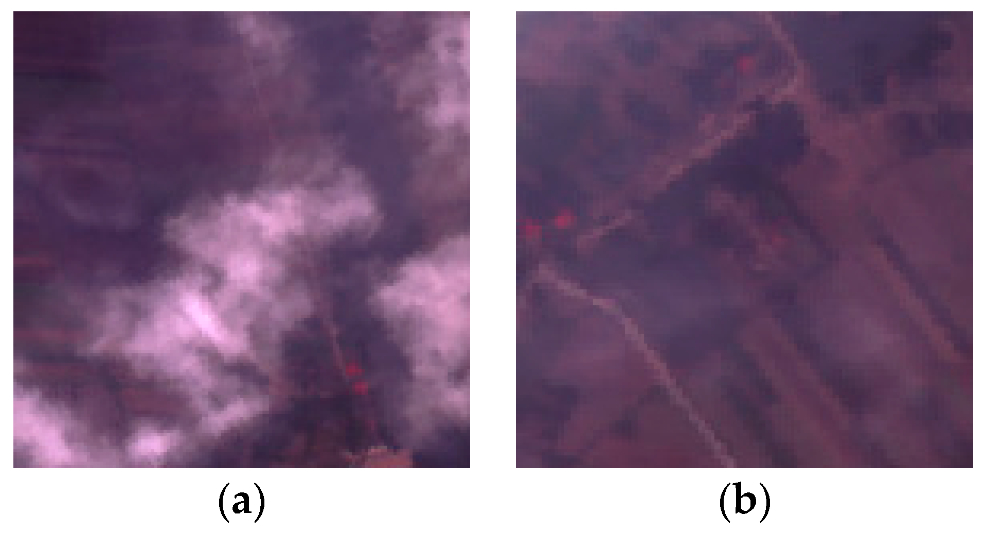
2.2. Typical Cloud Features
2.3. Feature Selection
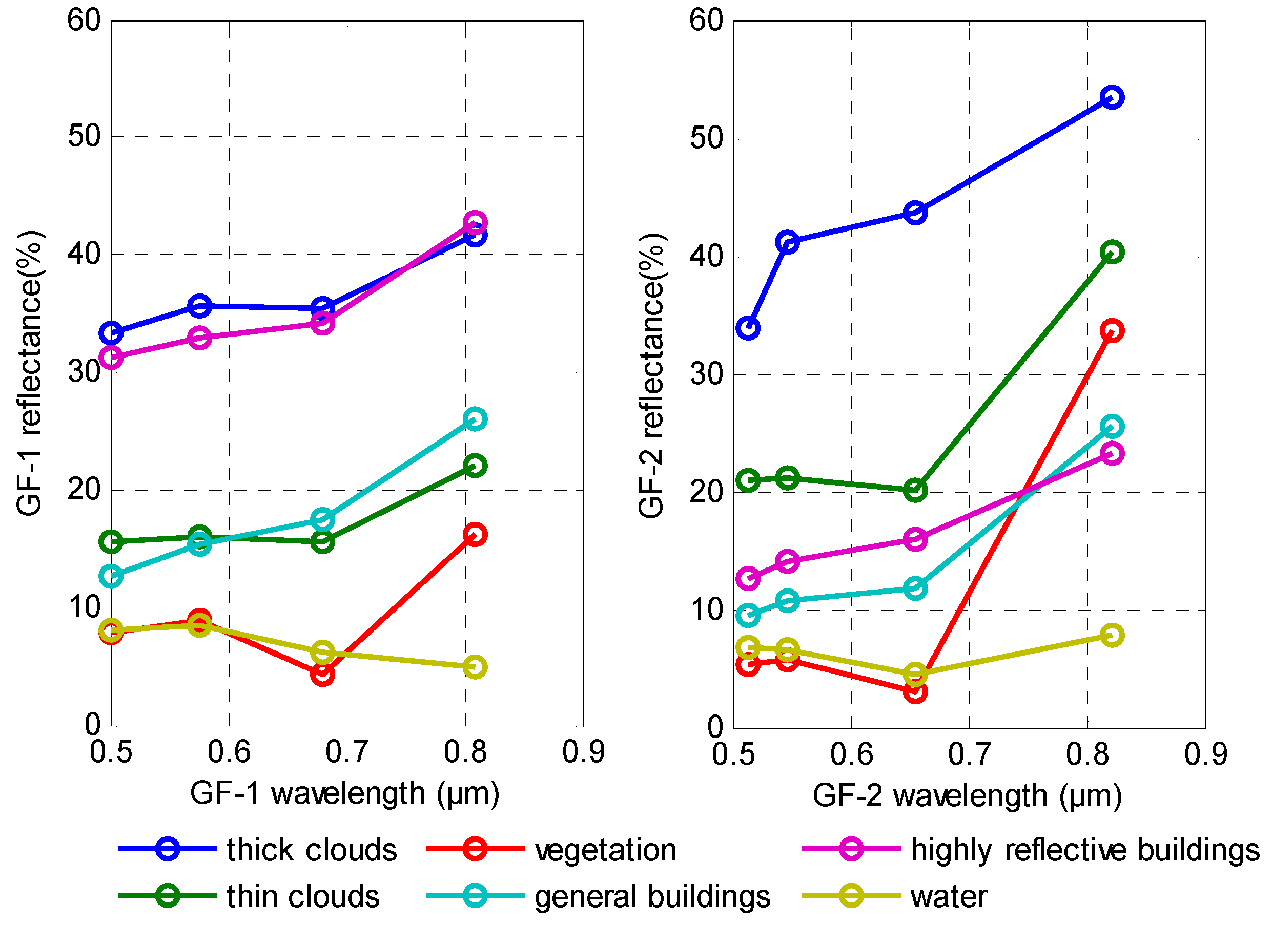
2.3.1. Selection of Spectral Features
2.3.2. Selection of Texture Features
2.3.3. Selection of Other Features
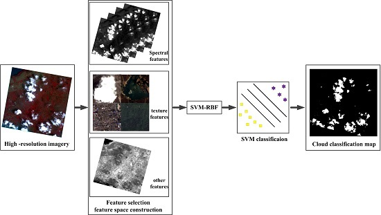
2.4. Methods
2.4.1. SVM Classification
2.4.2. Feature Fusion
2.4.3. SVM-Based Multi-Feature Fusion
3. Results
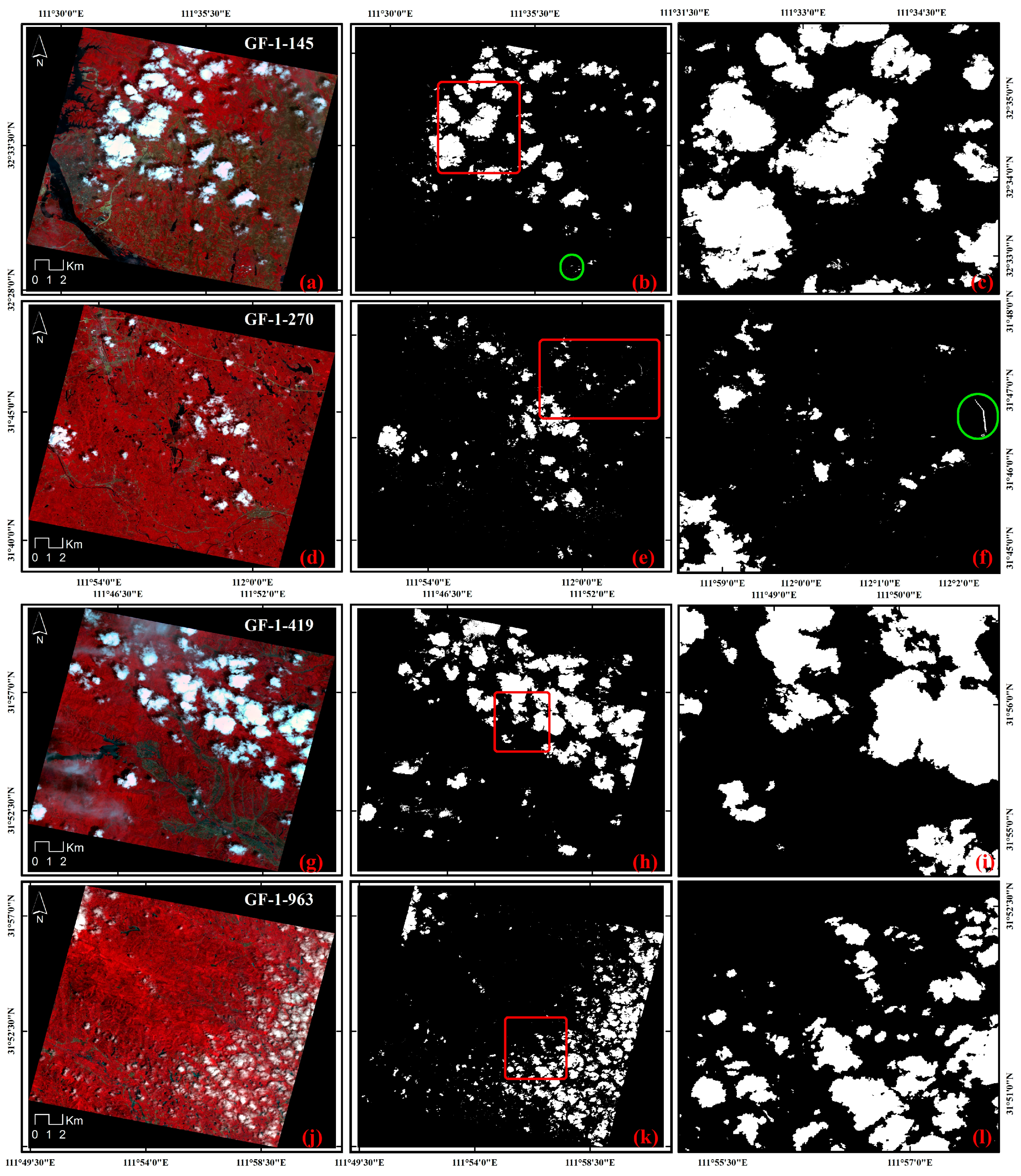
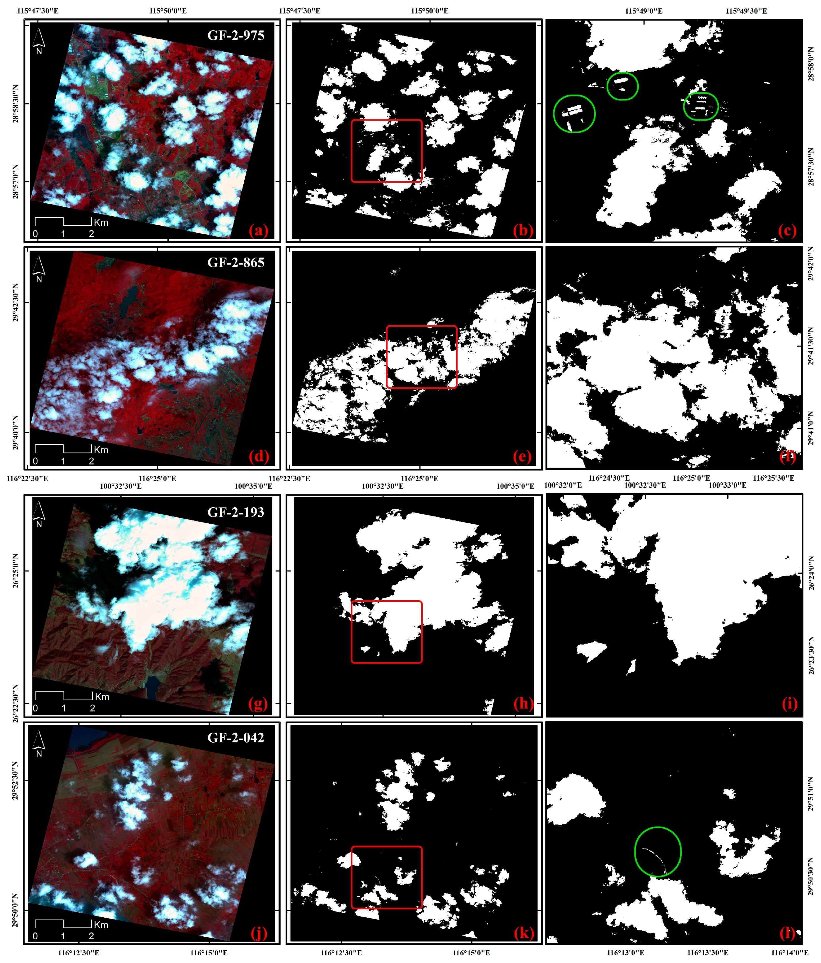
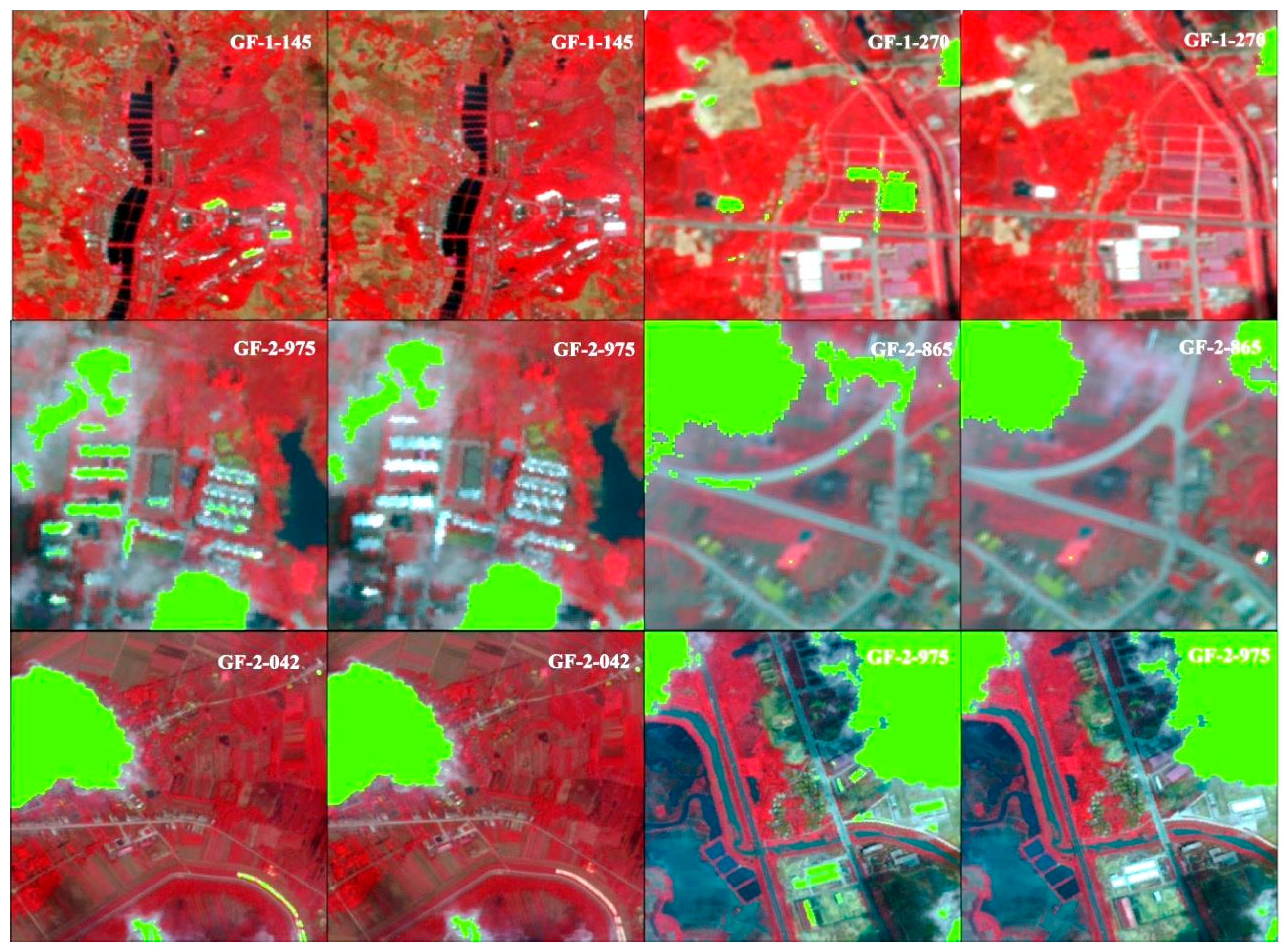
3.1. Cloud Detection Experiment
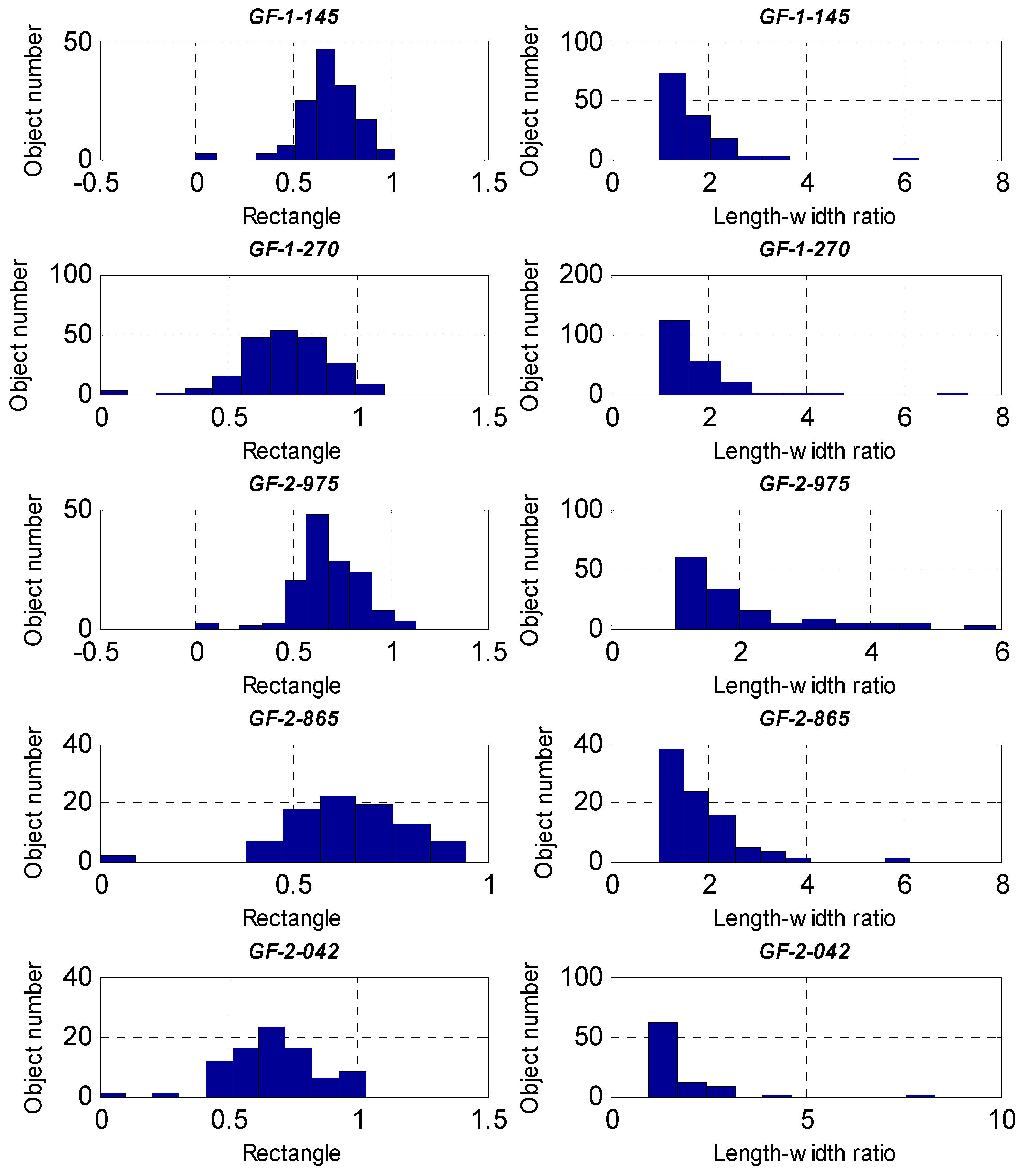
3.2. Object-Oriented Post-Processing
4. Discussion
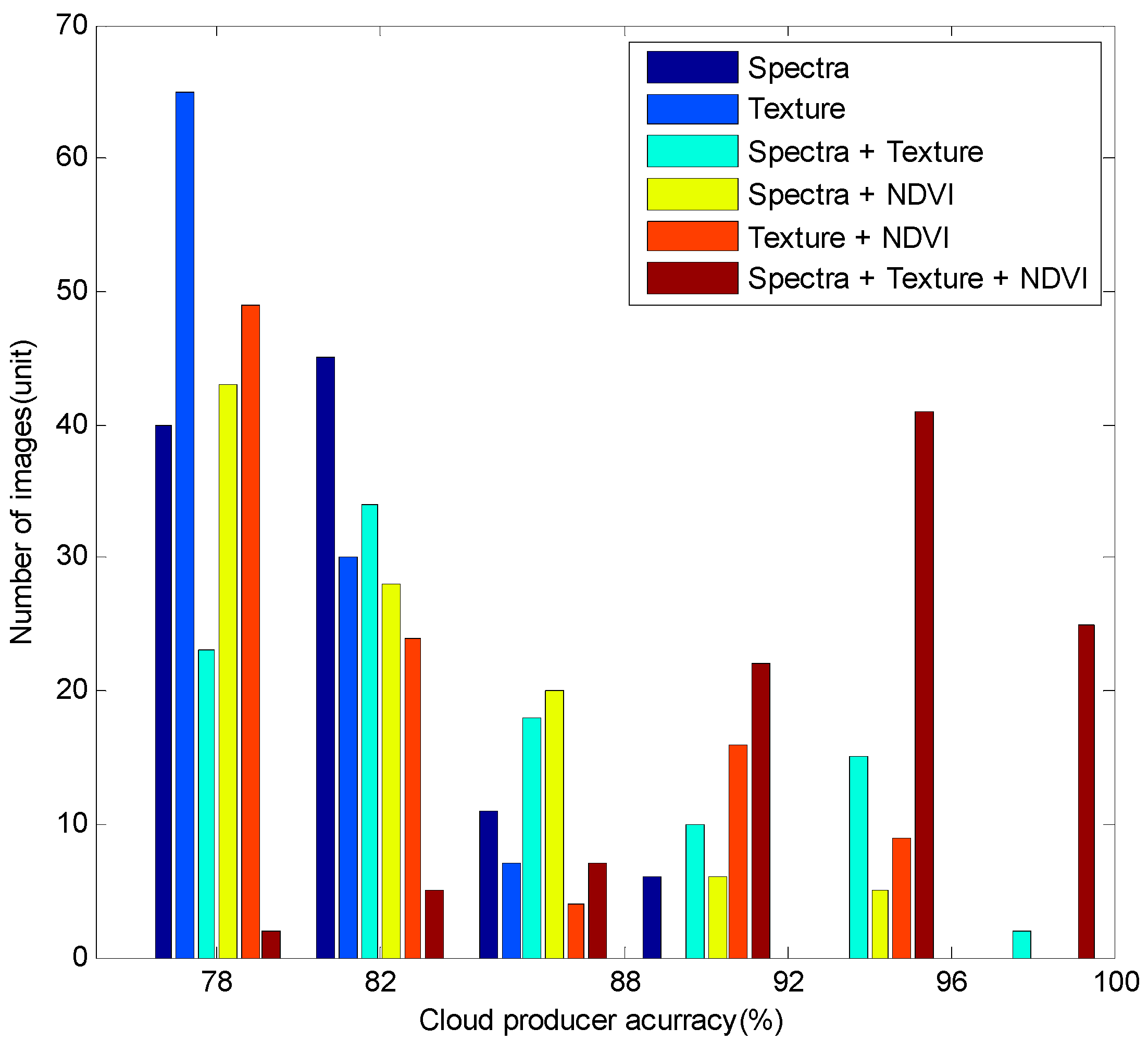
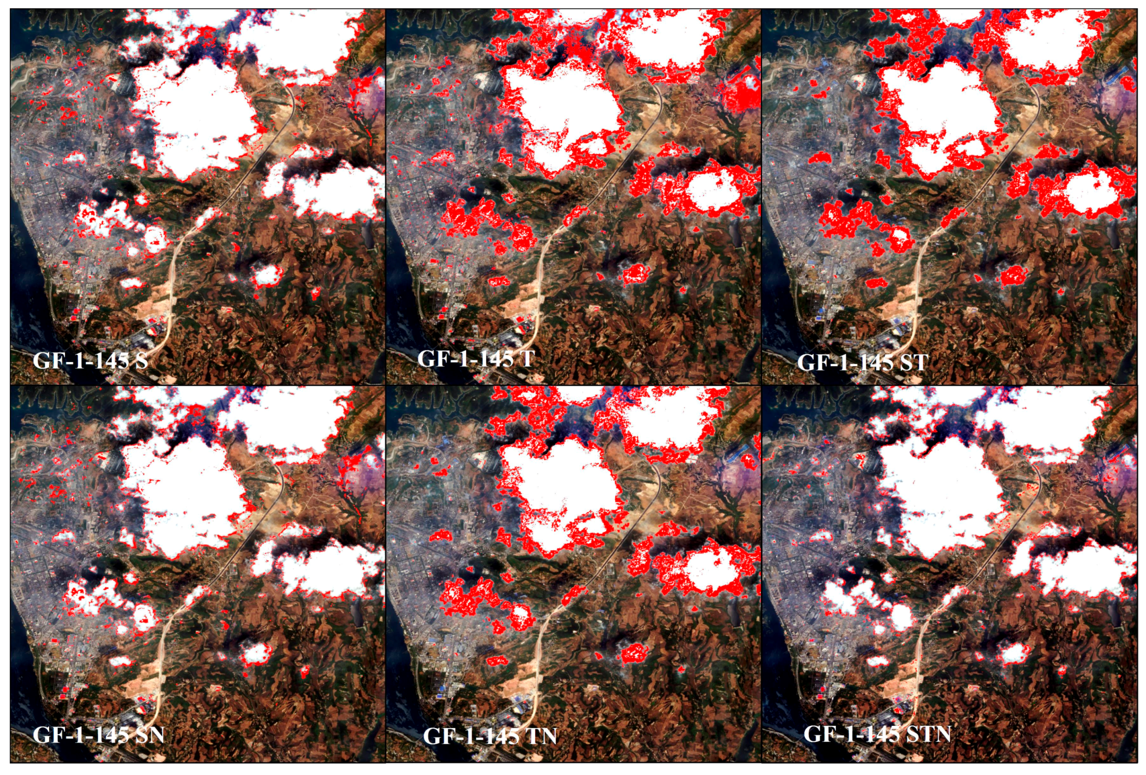
4.1. Accuracy Analysis of Multiple Features
4.2. The Scalability of the Algorithm
4.3. Summary of Advantages and Disadvantages
5. Conclusions
Acknowledgments
Author Contributions
Conflicts of Interest
References
- Roy, D.P.; Ju, J.; Kline, K.; Scaramuzza, P.L.; Kovalskyy, V.; Hansen, M.; Loveland, T.R.; Vermote, E.; Zhang, C. Web-enabled landsat data (Weld): Landsat ETM+ composited mosaics of the conterminous United States. Remote Sens. Environ. 2010, 114, 35–49. [Google Scholar] [CrossRef]
- Zhu, Z.; Wang, S.; Woodcock, C.E. Improvement and expansion of the fmask algorithm: Cloud, cloud shadow, and snow detection for landsats 4–7, 8, and sentinel 2 images. Remote Sens. Environ. 2015, 159, 269–277. [Google Scholar] [CrossRef]
- Shi, C.; Xie, Z. Operational method of total precipitable water retrieved from satellite multi-channels’ infrared data. J. Infrared Millim. Waves 2005, 24, 304–308. [Google Scholar]
- Zhu, Z.; Woodcock, C.E. Object-based cloud and cloud shadow detection in landsat imagery. Remote Sens. Environ. 2012, 118, 83–94. [Google Scholar] [CrossRef]
- Huang, C.; Thomas, N.; Goward, S.N.; Masek, J.G.; Zhu, Z.; Townshend, J.R.; Vogelmann, J.E. Automated masking of cloud and cloud shadow for forest change analysis using landsat images. Int. J. Remote Sens. 2010, 31, 5449–5464. [Google Scholar] [CrossRef]
- Sedano, F.; Kempeneers, P.; Strobl, P.; Kucera, J.; Vogt, P.; Seebach, L.; San-Miguel-Ayanz, J. A cloud mask methodology for high resolution remote sensing data combining information from high and medium resolution optical sensors. ISPRS J. Photogramm. Remote Sens. 2011, 66, 588–596. [Google Scholar] [CrossRef]
- Tseng, D.-C.; Tseng, H.-T.; Chien, C.-L. Automatic cloud removal from multi-temporal spot images. Appl. Math. Comput. 2008, 205, 584–600. [Google Scholar] [CrossRef]
- Han, Y.; Kim, B.; Kim, Y.; Lee, W.H. Automatic cloud detection for high spatial resolution multi-temporal images. Remote Sens. Lett. 2014, 5, 601–608. [Google Scholar] [CrossRef]
- Lu, D. Detection and substitution of clouds/hazes and their cast shadows on ikonos images. Int. J. Remote Sens. 2007, 28, 4027–4035. [Google Scholar] [CrossRef]
- Marais, I.V.Z.; Du Preez, J.A.; Steyn, W.H. An optimal image transform for threshold-based cloud detection using heteroscedastic discriminant analysis. Int. J. Remote Sens. 2011, 32, 1713–1729. [Google Scholar] [CrossRef]
- Fisher, A. Cloud and cloud-shadow detection in spot5 hrg imagery with automated morphological feature extraction. Remote Sens. 2014, 6, 776–800. [Google Scholar] [CrossRef]
- Lakshmanan, V.; DeBrunner, V.; Rabin, R. Texture-based segmentation satellite weather imagery. In Proceedings of the 2000 International Conference on Image Processing, Vancouver, BC, Canada, 10–13 September 2000.
- Walder, P.; MacLaren, I. Neural network based methods for cloud classification on AVHRR images. Int. J. Remote Sens. 2000, 21, 1693–1708. [Google Scholar] [CrossRef]
- Tian, B.; Azimi-Sadjadi, M.R.; Vonder Haar, T.H.; Reinke, D. Temporal updating scheme for probabilistic neural network with application to satellite cloud classification. IEEE Trans. Neural Netw. 2000, 11, 903–920. [Google Scholar] [CrossRef] [PubMed]
- Simpson, J.J.; Gobat, J.I. Improved cloud detection in goes scenes over the oceans. Remote Sens. Environ. 1995, 52, 79–94. [Google Scholar] [CrossRef]
- Chen, F.; Yan, D.; Zhao, Z. Haze detection and removal in remote sens.ing images based on undecimated wavelet transform. Geo. Inf. Sci. Wuhan Univ. 2007, 1, 71–74. [Google Scholar]
- Addesso, P.; Conte, R.; Longo, M.; Restaino, R.; Vivone, G. Svm-Based cloud detection aided by contextual information. In Proceedings of the 2012 Tyrrhenian Workshop on Advances in Radar and Remote Sensing (TyWRRS), Wessling, Germany, 12–14 September 2012.
- Dell’Acqua, F.; Gamba, P.; Ferrari, A.; Palmason, J.; Benediktsson, J.; Arnason, K. Exploiting spectral and spatial information in hyperspectral urban data with high resolution. IEEE Geosci. Remote Sens. Lett. 2004, 1, 322–326. [Google Scholar] [CrossRef]
- Li, H.-Q.; Liu, Z.-K.; Lin, F. Aerial image classification method based on fractal theory. J. Remote Sens 2001, 5, 353–357. [Google Scholar]
- Benediktsson, J.A.; Palmason, J.A.; Sveinsson, J.R. Classification of hyperspectral data from urban areas based on extended morphological profiles. IEEE Trans. Geosci. Remote Sens. 2005, 43, 480–491. [Google Scholar] [CrossRef]
- Duro, D.C.; Franklin, S.E.; Dubé, M.G. A comparison of pixel-based and object-based image analysis with selected machine learning algorithms for the classification of agricultural landscapes using spot-5 HRG imagery. Remote Sens. Environ. 2012, 118, 259–272. [Google Scholar] [CrossRef]
- Foody, G.M. The effect Mis-Labeled Training Data on the Accuracy Supervised Image Classification by Svm. In Proceedings of the 2015 IEEE International Geoscience and Remote Sensing Symposium (IGARSS), Milan, Italy, 26–31 July 2015.
- Huang, X.; Zhang, L. An svm ensemble approach combining spectral, structural, and semantic features for the classification of high-resolution remotely sensed imagery. IEEE Trans. Geosci. Remote Sens. 2013, 51, 257–272. [Google Scholar] [CrossRef]
- Pasolli, E.; Melgani, F.; Tuia, D.; Pacifici, F.; Emery, W.J. SVM active learning approach for image classification using spatial information. IEEE Trans. Geosci. Remote Sens. 2014, 52, 2217–2233. [Google Scholar] [CrossRef]
- Ciresan, D.; Meier, U.; Schmidhuber, J. Multi-Column Deep Neural Networks For image Classification. In Proceedings of the 2012 IEEE Conference on Computer Vision and Pattern Recognition (CVPR), Rama Chellappa, RI, USA, 16–21 June 2012.
- Kussul, N.; Skakun, S.; Kussul, O. Comparative analysis of neural networks and statistical approaches to remote sensing image classification. Int. J. Comput. 2014, 5, 93–99. [Google Scholar]
- Li, L.; Chen, Y.; Yu, X.; Liu, R.; Huang, C. Sub-pixel flood inundation mapping from multispectral remotely sensed images based on discrete particle swarm optimization. ISPRS J. Photogramm. Remote Sens. 2015, 101, 10–21. [Google Scholar] [CrossRef]
- Wang, H.; He, Y.; Guan, H. Application support vector machines in cloud detection using EOS/MODIS. In Proceedings of the Remote Sensing Applications for Aviation Weather Hazard Detection and Decision Support, San Diego, CA, USA, 25 August 2008.
- Hughes, M.J.; Hayes, D.J. Automated detection of cloud and cloud shadow in single-date landsat imagery using neural networks and spatial post-processing. Remote Sens. 2014, 6, 4907–4926. [Google Scholar] [CrossRef]
- Chethan, H.; Raghavendra, R.; Kumar, G.H. Texture based approach for cloud classification using svm. In Proceedings of the International Conference on Advances in Recent Technologies in Communication and Computing, Kottayam, Kerala, India, 27–28 October 2009.
- Baseski, E.; Cenaras, C. Texture color based cloud detection. In Proceedings of the 2015 7th International Conference on Recent Advances in Space Technologies (RAST), Istanbul, Turkey, 16–19 June 2015.
- Latry, C.; Panem, C.; Dejean, P. Cloud detection with svm technique. In Proceedings of the IEEE International Geoscience and Remote Sensing Symposium, IGARSS 2007, Barcelona, Spain, 23–27 July 2007.
- Wyatt, C. Radiometric Calibration: Theory Methods; Elsevier: New York, NY, USA, 2012. [Google Scholar]
- Teillet, P. Image correction for radiometric effects in remote sensing. Int. J. Remote Sens. 1986, 7, 1637–1651. [Google Scholar] [CrossRef]
- Kaufman, Y.J.; Sendra, C. Algorithm for automatic atmospheric corrections to visible and near-ir satellite imagery. Int. J. Remote Sens. 1988, 9, 1357–1381. [Google Scholar] [CrossRef]
- Guide, E.U. Atmospheric correction module: Quac and flaash user’s guide. Version 2009, 4, 1–44. [Google Scholar]
- Schiller, H.; Brockmann, C.; Krasemann, H.; Schönfeld, W. A method for detection and classification of clouds over water. In Proceedings of the 2nd MERIS/(A)ATSR User Workshop, Frascati, Italy, 22–26 September 2008.
- Xiao, Z. Study on Cloud Detection Method for High Resolution Satellite Remote Sensoring Image; Harbin Institute of Technology: Heilongjiang, China, 2013. [Google Scholar]
- Bajwa, I.S.; Naweed, M.; Asif, M.N.; Hyder, S.I. Feature based image classification by using principal component analysis. ICGST Int. J. Graph. Vis. Image Process. GVIP 2009, 9, 11–17. [Google Scholar]
- Haralick, R.M.; Shanmugam, K.; Dinstein, I.H. Textural features for image classification. IEEE Trans. Syst. Man Cybern. 1973, 3, 610–621. [Google Scholar] [CrossRef]
- Pesaresi, M.; Gerhardinger, A.; Kayitakire, F. A robust built-up area presence index by anisotropic rotation-invariant textural measure. IEEE J. Sel. Top. Appl. Earth Obs. Remote Sens. 2008, 1, 180–192. [Google Scholar] [CrossRef]
- Ouma, Y.O.; Tetuko, J.; Tateishi, R. Analysis of co-occurrence and discrete wavelet transform textures for differentiation of forest and non-forest vegetation in very-high-resolution optical-sensor imagery. Int. J. Remote Sens. 2008, 29, 3417–3456. [Google Scholar] [CrossRef]
- Puissant, A.; Hirsch, J.; Weber, C. The utility of texture analysis to improve per-pixel classification for high to very high spatial resolution imagery. Int. J. Remote Sens. 2005, 26, 733–745. [Google Scholar] [CrossRef]
- Anys, H.; Bannari, A.; He, D.; Morin, D. Texture analysis for the mapping urban areas using airborne meis-ii Images. In Proceedings of the First International Airborne Remote Sensing Conference and Exhibition, Strasbourg, France, 12–15 September 1994.
- Chang, C.-C.; Lin, C.-J. Libsvm: A library for support vector machines. ACM Trans. Int. Sys. Tech. 2011. [Google Scholar] [CrossRef]
- Mountrakis, G.; Im, J.; Ogole, C. Support vector machines in remote sensing: A review. ISPRS J. Photogramm. Remote Sens. 2011, 66, 247–259. [Google Scholar] [CrossRef]
- Paneque-Gálvez, J.; Mas, J.-F.; Moré, G.; Cristóbal, J.; Orta-Martínez, M.; Luz, A.C.; Guèze, M.; Macía, M.J.; Reyes-García, V. Enhanced land use/cover classification of heterogeneous tropical landscapes using support vector machines and textural homogeneity. Int. J. Appl. Earth Obs. Geoinf. 2013, 23, 372–383. [Google Scholar] [CrossRef]
- Anantrasirichai, N.; Achim, A.; Morgan, J.E.; Erchova, I.; Nicholson, L. Svm-Based texture classification in optical coherence tomography. In Proceedings of the 2013 IEEE 10th International Symposium onBiomedical Imaging (ISBI), San Francisco, CA, USA, 7–11 April 2013.
- Cristianini, N.; Shawe-Taylor, J. An Introduction to Support Vector Machines Other Kernel-Based Learning Methods; Cambridge University Press: Cambridge, UK, 2000. [Google Scholar]
- Christodoulou, C.; Michaelides, S.C.; Pattichis, C.S. Multifeature texture analysis for the classification of clouds in satellite imagery. IEEE Trans. Geosci. Remote Sens. 2003, 41, 2662–2668. [Google Scholar] [CrossRef]
- Wu, X.; Peng, J.; Shan, J.; Cui, W. Evaluation of semivariogram features for object-based image classification. Geo-Spat. Inf. Sci. 2015, 18, 159–170. [Google Scholar] [CrossRef]
- Dubuisson-Jolly, M.-P.; Gupta, A. Color and texture fusion: Application to aerial image segmentation and gis updating. Image Vis. Comput. 2000, 18, 823–832. [Google Scholar] [CrossRef]
- Bai, X.; Liu, C.; Ren, P.; Zhou, J.; Zhao, H.; Su, Y. Object classification via feature fusion based marginalized kernels. IEEE Geosci. Remote Sens. Lett. 2015, 12, 8–12. [Google Scholar]
- Hong, Z. Digital Image Processing; Science Press: Beijing, China, 2005. [Google Scholar]
- Yuan, Y.; Hu, X. Bag-of-words and object-based classification for cloud extraction from satellite imagery. IEEE J. Sel. Top. Appl. Earth Obs. Remote Sens. 2015, 8, 4197–4205. [Google Scholar] [CrossRef]


| Abbreviation/Image Information | High Resolution Image Date | Solar Zenith Angle (Degree) | Cloud Types | Scene Description |
|---|---|---|---|---|
| GF-1-145 L1A0000232145 | 22 May 2014 | 73.6156 | Medium, low density clouds | Agriculture, high reflectance buildings and road |
| GF-1-270 L1A0000268270 | 6 July 2014 | 74.5897 | Medium, low density clouds | vegetation, high reflectance buildings and road |
| GF-1-419 L1A0000232419 | 22 May 2014 | 74.1973 | Medium, high density clouds | Mountainous area with high reflectance bare soil slope |
| GF-1-963 L1A0000264963 | 2 July 2014 | 75.0930 | Small, high density clouds | Mountainous area with high reflectance bare soil slope |
| GF-2-865 L1A0001028865 | 21 May 2015 | 17.6541 | Large clouds | Urban area with high reflectance buildings and road |
| GF-2-193 L1A0001451193 | 5 March 2016 | 36.4954 | Large clouds | Mountainous area with high reflectance bare soil slope |
| GF-2-042 L1A0000836042 | 31 May 2015 | 16.4647 | Medium, low density clouds | Agriculture, high reflectance buildings and road |
| GF-2-975 L1A0000835975 | 31 May 2015 | 16.4336 | Medium, high density clouds | Agriculture, high reflectance buildings and road |
| Features | Feature Space |
|---|---|
| Spectral features | Band 1, Band 2, Band 3, Band 4 |
| Texture features | Mean, Variance, Homogeneity, Contrast, Correlation, Entropy |
| Window Size | |
| Band selection: PC1 and PC2 | |
| Other features | NDVI |
| Sensor | Types | Training Samples |
|---|---|---|
| GF-1-145 | Cloud | 2207 |
| Non-cloud | 5444 | |
| GF-1-270 | Cloud | 2043 |
| Non-cloud | 5722 | |
| GF-1-419 | Cloud | 2714 |
| Non-cloud | 5671 | |
| GF-1-963 | Cloud | 2565 |
| Non-cloud | 5672 | |
| GF-2-865 | Cloud | 2041 |
| Non-cloud | 5365 | |
| GF-2-193 | Cloud | 2423 |
| Non-cloud | 5325 | |
| GF-2-042 | Cloud | 2356 |
| Non-cloud | 5671 | |
| GF-2-975 | Cloud | 2456 |
| Non-cloud | 5432 |
| Sensor | Overall Accuracy | Kappa Coefficient | Post Processing Accuracy |
|---|---|---|---|
| GF-1-145 | 96.6791% | 0.8992 | 97.5263% |
| GF-1-270 | 95.4259% | 0.8936 | 97.6589% |
| GF-2-975 | 95.2362% | 0.8363 | 96.6701% |
| GF-2-865 | 96.6252% | 0.9109 | 96.7713% |
| GF-2-042 | 96.4454% | 0.9179 | 97.6235% |
| Cloud User Accuracy | 76%–80% | 80%–84% | 84%–88% | 88%–92% | 92%–96% | 96%–100% | The Average Accuracy |
|---|---|---|---|---|---|---|---|
| S | 40 | 45 | 11 | 6 | 0 | 0 | 83.33% |
| T | 65 | 30 | 7 | 0 | 0 | 0 | 81.76% |
| ST | 23 | 34 | 18 | 10 | 15 | 2 | 84.17% |
| SN | 43 | 28 | 20 | 6 | 5 | 0 | 86.67% |
| TN | 49 | 24 | 4 | 16 | 9 | 0 | 84.55% |
| STN | 2 | 5 | 7 | 22 | 41 | 25 | 93.67% |
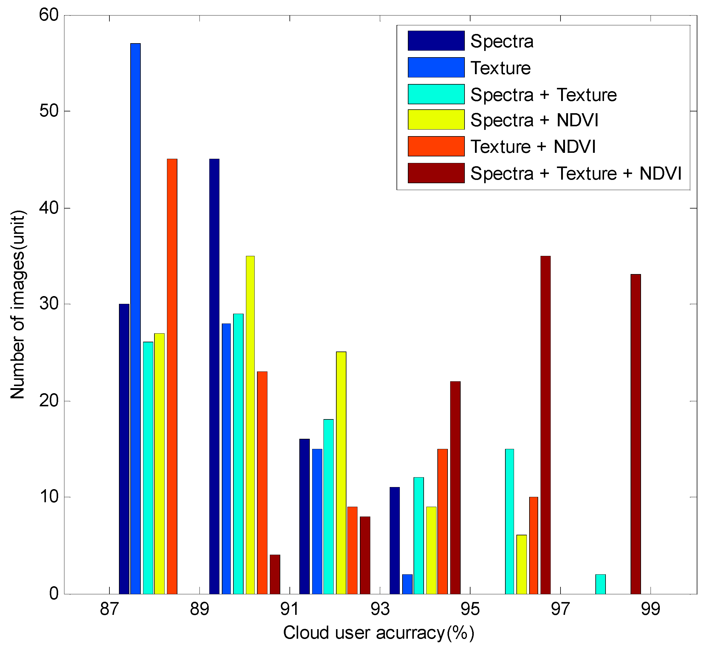
| Cloud User Accuracy | 86%–88% | 88%–90% | 90%–92% | 92%–94% | 94%–96% | 96%–98% | The Average Accuracy |
|---|---|---|---|---|---|---|---|
| S | 29 | 45 | 16 | 11 | 1 | 0 | 90.16% |
| T | 57 | 28 | 15 | 2 | 0 | 0 | 89.25% |
| ST | 26 | 29 | 18 | 12 | 15 | 2 | 91.35% |
| SN | 27 | 35 | 25 | 9 | 6 | 0 | 90.67% |
| TN | 45 | 23 | 9 | 15 | 10 | 0 | 90.47% |
| STN | 0 | 4 | 8 | 22 | 35 | 33 | 95.67% |
© 2016 by the authors; licensee MDPI, Basel, Switzerland. This article is an open access article distributed under the terms and conditions of the Creative Commons Attribution (CC-BY) license (http://creativecommons.org/licenses/by/4.0/).
Share and Cite
Bai, T.; Li, D.; Sun, K.; Chen, Y.; Li, W. Cloud Detection for High-Resolution Satellite Imagery Using Machine Learning and Multi-Feature Fusion. Remote Sens. 2016, 8, 715. https://doi.org/10.3390/rs8090715
Bai T, Li D, Sun K, Chen Y, Li W. Cloud Detection for High-Resolution Satellite Imagery Using Machine Learning and Multi-Feature Fusion. Remote Sensing. 2016; 8(9):715. https://doi.org/10.3390/rs8090715
Chicago/Turabian StyleBai, Ting, Deren Li, Kaimin Sun, Yepei Chen, and Wenzhuo Li. 2016. "Cloud Detection for High-Resolution Satellite Imagery Using Machine Learning and Multi-Feature Fusion" Remote Sensing 8, no. 9: 715. https://doi.org/10.3390/rs8090715
APA StyleBai, T., Li, D., Sun, K., Chen, Y., & Li, W. (2016). Cloud Detection for High-Resolution Satellite Imagery Using Machine Learning and Multi-Feature Fusion. Remote Sensing, 8(9), 715. https://doi.org/10.3390/rs8090715