1. Introduction
Sea ice affects the exchange of heat, energy, mass, and momentum between the atmosphere and ocean, and has a significant impact on society in terms of marine transportation, security, fisheries, hazards, recreation, and hunting. Quantifying its variability in space and time is critical for improving our understanding of climate sensitivity at high latitudes [
1,
2,
3,
4,
5]. As noted in the Integrated Global Observing Strategy Cryosphere Theme Report [
6], “Adequate knowledge of the sea ice mass is important for weather and climate prediction, assessment and prediction of navigation, shipping, fishing, mineral resource exploration and exploitation, and in many other practical applications. The sea ice also provides indicators of climate change, yet it may be the most under-sampled domain in the climate system”.
Sea ice cover, generally reported as extent or area, has been monitored from space for decades and it is commonly used in assessing changes in the Arctic climate system. However, from both thermodynamic and dynamic perspectives, sea ice thickness provides more information than area or extent [
7]. Unfortunately, ice thickness is difficult to measure from space, and in situ observations are sparse. Until recently, available sea ice thickness data have been limited to observations from aircraft flights, submarine sonar, offshore station measurements, and upward-looking sonar from moorings and field campaigns. While these data sets have proven invaluable, they are generally too limited in space and time to capture variability over the entire sea ice-covered area on scales sufficient for studies of climate change. Sea ice models and new satellite products provide the desired temporal and spatial coverage, but their accuracy has not been fully assessed.
One of the advances in this area was the estimation of ice freeboard and thickness from the Ice, Cloud, and land Elevation Satellite (ICESat) Geoscience Laser Altimeter System (GLAS) [
8]. These products, available for 2003–2008, cover much of the Arctic and Antarctic. Unfortunately, the data record is relatively short, as data acquisition ended in October 2009 due to the failure of GLAS. Comparable LIDAR-derived freeboard and thicknesses will not be acquired again until the launch of ICESat-2 planned for 2018. The NASA IceBridge aircraft campaign is helping fill the gap between ICESat and ICESat-2, but the flights are limited in spatial and temporal coverage [
9]. The European Space Agency’s (ESA) Cryosat-2 satellite, launched in 2011 with a radar altimeter, is now providing ice thickness estimates in a manner similar to that of ICESat [
10]. ESA’s Soil Moisture and Ocean Salinity (SMOS) mission launched in 2010 provides another satellite-retrieved sea ice thickness dataset, though it is for thin ice only [
11]. The differences between ICESat, IceBridge, submarine sonar, airborne electromagnetic induction, and in situ ice thickness data were examined in [
12].
The potential now exists to address the need for inter-decadal and consistent sea ice thickness estimates using the newly developed One-dimensional Thermodynamic Ice Model (OTIM) [
13]. OTIM utilizes data from optical (visible, near-infrared, and thermal infrared) satellite instruments such as the Advanced Very High Resolution Radiometer (AVHRR) onboard National Oceanic and Atmospheric Administration (NOAA) family of Polar-orbiting Operational Environmental Satellites (POES), and is incorporated in the AVHRR Polar Pathfinder–extended (APP-x) dataset that covers the period 1982 through the present [
14]. This is a very different approach than those used with ICESat, Cryosat-2, IceBridge, and SMOS. Altimeters provide measurements of the ice elevation and hence the thickness of the ice/snow layer above the water level (freeboard). SMOS employs the relationship between passive microwave brightness temperatures and ice thickness. In contrast, the OTIM approach estimates the ice thickness through a complex formulation of the surface energy budget using various satellite-derived variables as input. It is, therefore, a different and less direct approach than with altimeters.
In this paper, we examine the similarities and differences between the satellite and aircraft sea ice thickness products for the Arctic. Ice thickness from the Pan-Arctic Ice Ocean Modeling and Assimilation System (PIOMAS) is also included. The intercomparison is complicated by the fact that the datasets cover different time periods and have different temporal and spatial resolutions, with APP-x and PIOMAS having the longest, multi-decadal record. Comparisons are therefore done for the periods of overlap. It is not our intention to recommend one product over the others as some, notably CryoSat-2 and SMOS, have not yet reached a high level of maturity. Instead, we focus on their similarities and differences.
2. Description of Data Sets
There are six sea ice thickness datasets used in this study. Four of six datasets are based on satellite data: APP-x [
14], ICESat GLAS laser altimeter [
8], CryoSat-2 radar altimeter [
10], and SMOS low-frequency passive microwave [
11,
15]. The other two ice thickness datasets are from the PIOMAS model [
16] and the IceBridge aircraft campaign [
9].
2.1. APP-x
The APP-x dataset includes cloud fraction, cloud optical depth, cloud particle phase and size, cloud top pressure and temperature, surface skin temperature, surface broadband albedo, sea ice thickness, radiative fluxes, and cloud radiative effects [
14]. APP-x consists of twice-daily composites at a 25 × 25 km
2 pixel size for the Arctic and Antarctic, currently over the period 1982–2014. Uncertainties in the APP-x data products are discussed and presented in [
17]. For identifying sea ice and calculating sea ice thickness with OTIM, sea ice concentration data used in this study are derived from Nimbus-7 Scanning Multi-channel Microwave Radiometer (SMMR) and Defense Meteorological Satellite Program (DMSP) -F8, -F11 and -F13 Special Sensor Microwave/Imager (SSM/I) radiances at a grid cell size of 25 × 25 km
2 using the NASA Team Algorithm. The ice concentration product is available from the National Snow and Ice Data Center (NSIDC) [
18].
OTIM is fully described in [
13]. It estimates ice thickness under the assumption of a surface energy balance at thermo-equilibrium, using an energy budget model with satellite-derived variables as input. All components of the surface energy budget are employed to estimate sea and lake ice thickness up to 5 m, though sensitivity studies show that the uncertainty increases by about 20% for ice greater than 3 m in thickness [
13]. It is capable of retrieving daytime and nighttime ice thickness under clear and cloudy conditions. It should be pointed out that the OTIM will not do ice thickness retrievals when the solar zenith angle is greater than 85 degrees and less than 91 degrees due to the large uncertainties of the input surface albedo, cloud mask, and surface shortwave radiation, and when the ice surface temperature is greater than the freezing point (~273 K depending on the sea water salinity). The accuracy of the input parameters, including snow depth, surface humidity, temperature, and wind, can significantly impact the accuracy of ice thickness calculations. The daytime retrieval is sensitive to ice and snow optical properties, and is therefore less reliable than the nighttime retrieval. Ice thickness is produced for each pixel that is identified as being ice covered. OTIM does not use the low-level satellite information (reflectances and brightness temperatures) directly, but rather uses other variables from the APP-x as well as built-in parameterization schemes for radiative fluxes. OTIM ice thickness validation studies were performed with sea ice thickness measurements from upward-looking sonar on submarines and moorings, as well as ground measurements. The overall accuracy (mean absolute bias) and uncertainty (root-mean-square difference, RMS) of the OTIM estimated ice thickness when compared to ground truth is approximately 0.20 m (less than 20%) and 0.54 m, respectively, over all types of sea ice.
2.2. ICESat
The Ice, Cloud, and land Elevation Satellite (ICESat) was launched on 13 January 2003 and was decommissioned from operations on 14 August 2010 [
19]. From 2003 to 2009, the ICESat mission provided the elevation data needed to determine sea ice thickness. Sea ice thickness derived from 25-km long segments in 10 ICESat campaigns are used here. The 10 campaigns span a period of 5 years, and were selected to provide representative sampling of the autumn and winter sea ice cover of the Arctic Ocean. Following [
8], the 10 campaign designations are ON03, FM04, ON04, FM05, ON05, FM06, ON06, MA07, ON07, and FM08. The campaign start dates vary by almost a month even though the length of laser operation, except for ON03, is approximately 34 days in each. The 10 campaigns were selected for the purpose of examining the inter-annual and seasonal variability in the retrieved sea ice thickness.
ICESat sea ice thickness is retrieved from estimated sea ice freeboard (the portion of surface elevation above sea water surface level) based on the GLAS elevation data with constructed snow cover data on the sea ice. As GLAS operates in the visible and near-infrared, it measures surface elevation at the snow-air interface in clear-sky conditions. More detailed descriptions and assessments of these retrieval algorithms are given in [
8]. The overall difference in sea ice draft between ICESat and moorings is less than 0.20 m [
19].
2.3. CryoSat-2
The CryoSat-2 satellite was launched in 2010 by the European Space Agency (ESA) for the purpose of measuring variations in the polar ice sheets and sea ice. The approach that CryoSat-2 employs to measure the sea ice thickness is very similar to that used for ICESat, which is to measure the freeboard of the ice/snow cover, and then estimate sea ice thickness. It is assumed that the radar signal penetrates to the snow-ice interface, though this is still a subject of investigation [
10]. This is an important difference between the two systems in that a laser altimeter signal is reflected essentially from the snow or bare ice surface, i.e., from the surface-air interface rather than the snow-ice interface [
8,
19].
The Alfred Wegener Institute (AWI)/Helmholtz Centre for Polar and Marine Research together with ESA maintain the sea ice thickness dataset from CryoSat-2. The Center for Polar Observation and Modelling (CPOM)/University College London also produces CryoSat-2 thickness estimates, including the quick-look datasets provided to the community [
20]. NASA Goddard Space Flight Center has also developed CryoSat-2 sea ice thickness product [
21]. The AWI data available on their website [
22] are used in this study. Currently only monthly data at a 25 km spatial resolution beginning in 2011 are available online. This dataset should not be considered as an operational product because the interpretation of CryoSat-2 radar signals for sea ice thickness is still under investigation. It is not, therefore, a fully calibrated and validated data product, but rather a research product for the scientific community.
2.4. SMOS
The Soil Moisture and Ocean Salinity (SMOS) satellite was launched on 2 November 2009 as a part of ESA’s Living Planet Programme. Its primary goal is to provide information on soil moisture on land and surface salinity in the ocean. It can also be used to retrieve information on sea ice, including sea ice thickness from the Microwave Imaging Radiometer with Aperture Synthesis (MIRAS) at an L-band frequency of 1.4 GHz. Sea ice thickness is derived from the brightness temperatures using a single-layer emissivity model. The emissivity is primarily a function of the bulk ice temperature, salinity, and thickness. The ice temperature is estimated from surface air temperature and a zero-dimensional thermodynamic model. Ice salinity is from a sea surface salinity weekly climatology. The sea ice thickness is corrected for the influence of the thickness distribution function. No correction is applied for ice concentration, so there will be an underestimation of ice thickness when open water is within the SMOS footprint. The method accounts for the thermodynamic influence of a parameterized snow layer on the ice temperature but does not account for the direct radiative effect of the snow. As SMOS brightness temperature is more sensitive to ice thicknesses less than 0.5 m, SMOS-derived ice thickness depends on the thin ice part of the ice thickness distribution within the field of view, while the contribution of the thicker ice part cannot be quantified due to the limited penetration depth and the saturation of SMOS brightness temperatures for thick ice, the maximum retrievable ice thickness is limited to about 1 m [
11].
SMOS sea ice thickness data are available from the Integrated Climate Data Center (ICDC) at the University of Hamburg in Germany. The 12.5 km SMOS daily Arctic sea ice thickness data covering the period 2010–2015 are available online [
23].
2.5. IceBridge
IceBridge is a NASA mission to provide airborne surveys of land and sea ice to bridge the gap between ICESat and ICESat-2. ICESat stopped data collection in 2009. ICESat-2 is planned for launch in mid-2018. IceBridge has been collecting sea ice and snow data since 2009 with instruments that include the Airborne Topographic Mapper (ATM) and a snow radar. The laser altimetry measurements from ATM are used to estimate sea ice thickness in a manner similar to that used for ICESat [
8]. The snow radar provides the snow depth on ice [
24]. The two different sensors onboard IceBridge measure surface elevation and snow depth separately and independently.
The IceBridge sea ice thickness final data products cover portions of the Arctic and Antarctic, 2009–2013, with a spatial resolution of 40 m. The data were obtained from the National Snow and Ice Data Center (NSIDC) [
25,
26]. A Quick Look dataset is available for parts of March and April, 2012–2015, and April–May in 2016. The Quick Look is an evaluation product for time-sensitive projects. Only the final product is used in this study.
Characteristics of the four satellite ice thickness products and the IceBridge thicknesses are summarized in
Table 1 from the relevant literature [
8,
9,
10,
11,
13,
15]. SMOS sea ice thickness uncertainty can be more than 1 meter when the thickness is greater than 0.50 m [
15], so the stated uncertainty is for thicknesses in the range 0~0.5 m. Regarding the IceBridge sea ice thickness, the uncertainty given in the table for a spatial resolution of 40 m is reduced to 0.40 m when averaged to a scale of 300 m [
9,
27].
2.6. PIOMAS
The Pan-Arctic Ice-Ocean Modeling and Assimilation System (PIOMAS) is a coupled ocean and sea ice model that assimilates daily sea ice concentration and sea surface temperature satellite products [
16]. PIOMAS couples the Parallel Ocean Program (POP) with a 12-category thickness and enthalpy distribution (TED) sea-ice model. The TED sea ice model is a dynamic thermodynamic model that originates from the Thorndike thickness distribution theory [
28] and was recently enhanced by enthalpy distribution theory [
29]. PIOMAS also calculates a 12-category snow depth distribution based on [
30]. Uncertainties in PIOMAS ice thickness and snow depth result mainly from the model forcing (wind, thermal, and precipitation forcing etc.), physics, and parameterizations [
31]. The PIOMAS dataset covers the period 1978 to the present, providing estimates of some key ice and ocean variables including Arctic sea ice thickness.
3. Analysis Methods
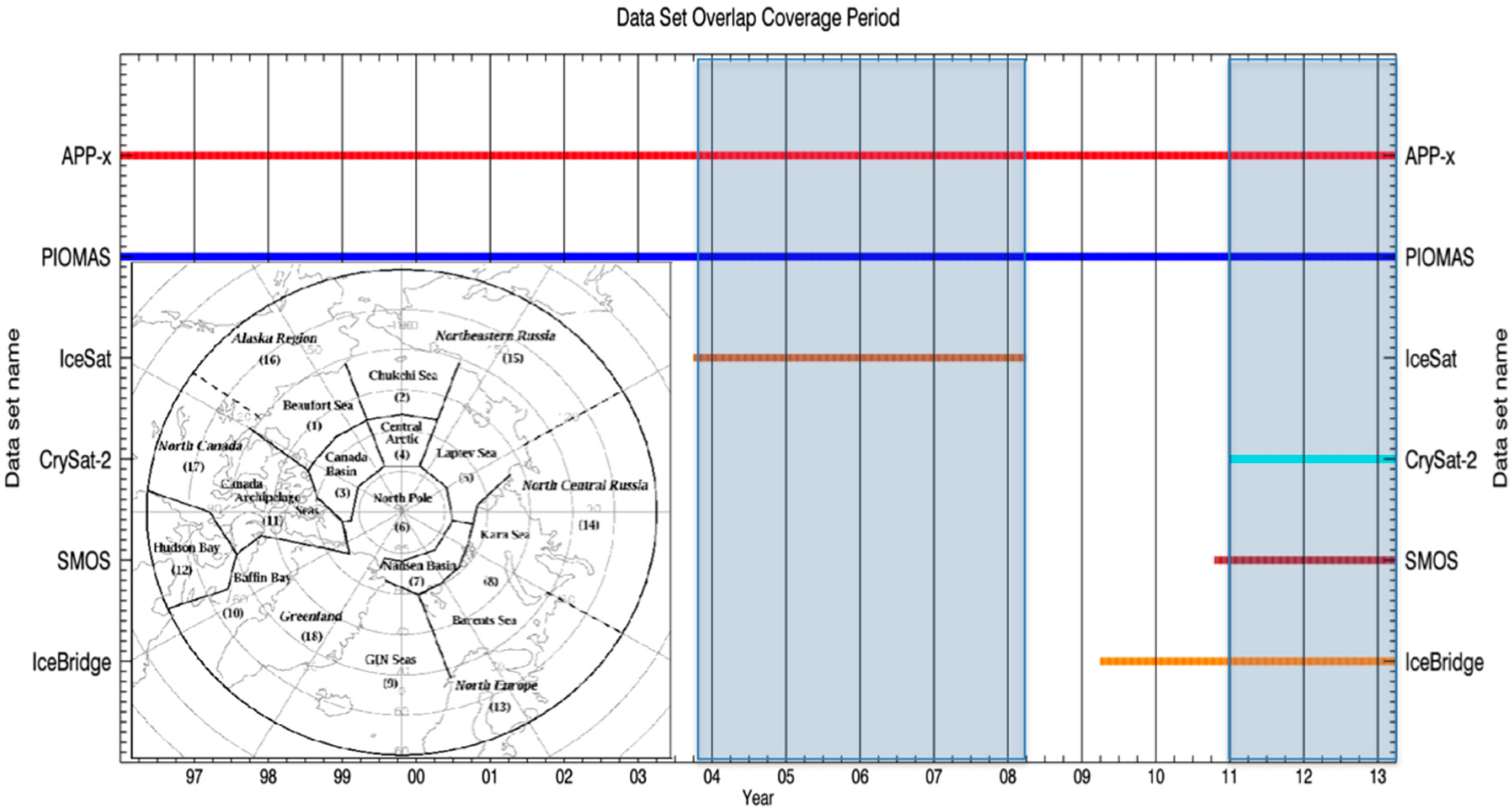
Sea ice thickness data from the six datasets described above have different temporal and spatial resolutions and time periods. The overlap periods of the six sea ice thickness datasets are shown in
Figure 1. In this study, three periods were selected for the inter-comparison: (1) an ICESat period from September 2003 to March 2008, utilizing data from February, March, October, and November; (2) a CryoSat-2 period from March 2011 to March 2013, utilizing data from March and October; and (3) an IceBridge period from March 2011 to March 2013, using data from March and April. These periods provide for the maximum data overlap.
All sea ice thickness datasets were first mapped to the Equal-Area Scalable Earth (EASE) grid to generate 25 km sea ice thickness data products. The daily data were then averaged to generate monthly means for each of the three comparison periods. Finally, six monthly mean sea ice thickness datasets on the 25 km EASE grid were generated.
The comparisons were done only for those grid cells that have valid values from each of the available datasets in each of the three periods. Descriptive statistics including the sample mean, standard deviations (STD), median, mode, and skewness were calculated for the datasets themselves and for their differences relative to the reference datasets. Histograms help interpret the non-Gaussian nature of the differences between the datasets. Correlation coefficients were calculated for each pair of the six datasets as another metric to evaluate their similarity, with corresponding P-values for the statistical significance.
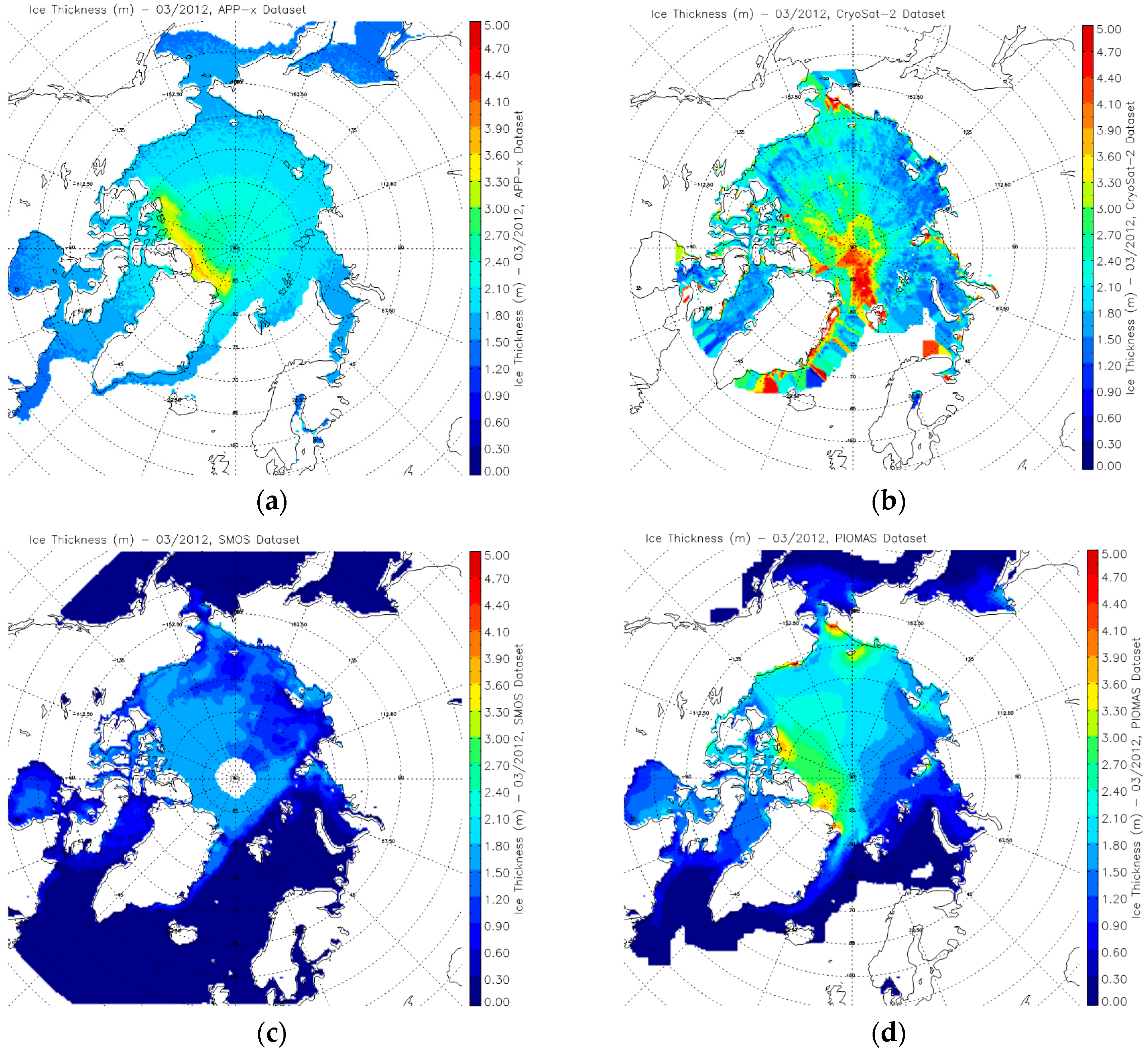
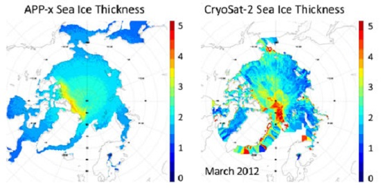
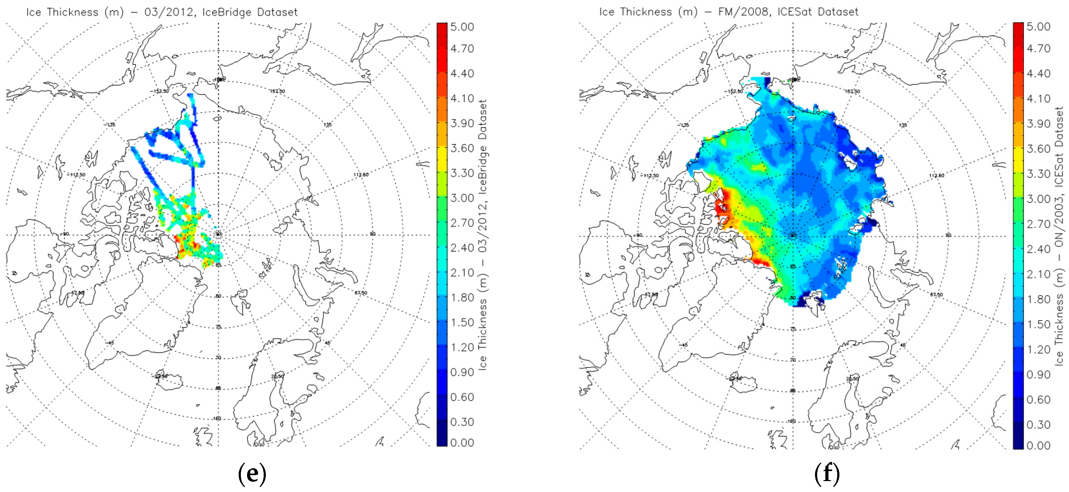
Figure 2 gives examples of the six sea ice thickness products for March 2012, except that the ICESat ice thickness example is a 34-day average for 2 February–31 March 2008.
4. Results
This section presents the inter-comparisons between datasets. Description statistics include the mean, standard deviation (STD), median, mode, skewness correlation coefficient. The term “bias” is used for the mean difference between datasets, although it is recognized that bias implies that the true value is known. We do not assume that any of the products are “truth”, but rather base the comparisons on a reference dataset for each of the three periods. For example, when ICESat is a reference dataset, “PIOMAS-ICESat” means the bias between PIOMAS and ICESat, i.e., the bias will be the mean of PIOMAS minus ICESat for all observations. The mode of the probability (or relative frequency) distribution of differences is the most frequently occurring value. The skewness is asymmetry of the distribution, which defines the extent to it differs from a Gaussian distribution. When the skewness is positive/negative, the right/left tail is longer and the mass of the distribution is concentrated on the left/right of the distribution figure.
4.1. ICESat Period
The ICESat period is from 23 September 2003 to 21 March 2008. It is composed of 10 campaign periods (see [
8], their
Table 1), which can be grouped into two sub-periods: the February-March (FM) winter period and the October–November (ON) autumn period over 6 years. During the ICESat period only APP-x and PIOMAS are available. The comparisons were done for the winter, autumn, and combined periods (FMON) between the three datasets.
As shown in
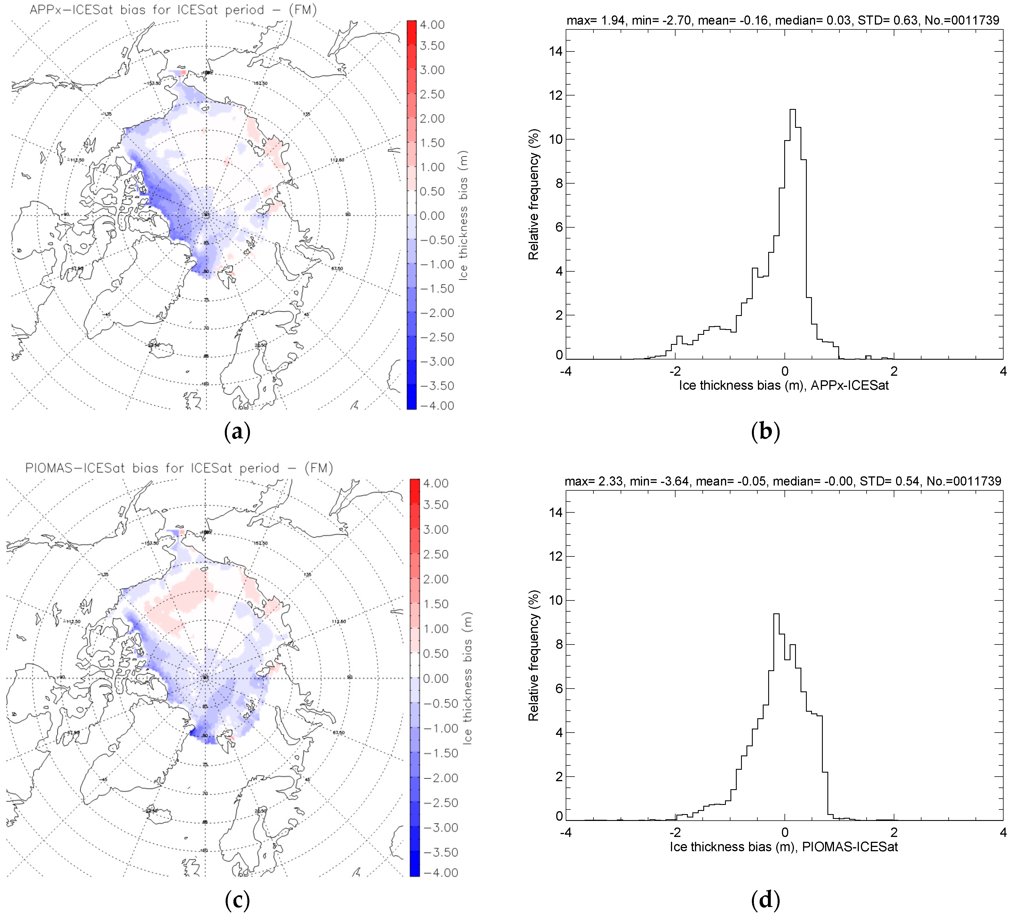
Figure 3 and
Table 2, the ICESat sea ice is thicker than APP-x and PIOMAS for both Winter (FM) and Autumn (ON) periods, especially for Autumn due to the very thick ICESat sea ice along the north coast of Greenland and the Canadian Archipelago. APP-x and PIOMAS ice in that area is relatively thinner. In contrast, in the thin sea ice areas of the Chukchi, Laptev, and Beaufort Seas, ICESat ice is thinner than APP-x and PIOMAS, but to a lesser extent than the reverse relationship in the northern Greenland and Canadian Archipelago area. Additionally, APP-x and PIOMAS show less spatial variation in comparison to ICESat. APP-x and PIOMAS are similar to each other with a correlation coefficient of 0.67 overall and a bias of the differences less than 8% (
Figure 4). The overall biases between APP-x and PIOMAS with ICESat are −0.48 m (−22%) and −0.31 m (−15%), respectively. In terms of the correlation coefficient, APP-x and ICESat are more similar for the winter period (FM), while PIOMAS and ICESat are more similar for the autumn period.
4.2. CryoSat-2 Period
The CryoSat-2 sea ice thickness data are available starting in 2011. Monthly mean data for March and October, 2011–2013 were used to maximize the overlap between datasets, though ICESat data are not available during this period. March over the Arctic is considered as the Winter period in this study; October is designated as the Autumn period.
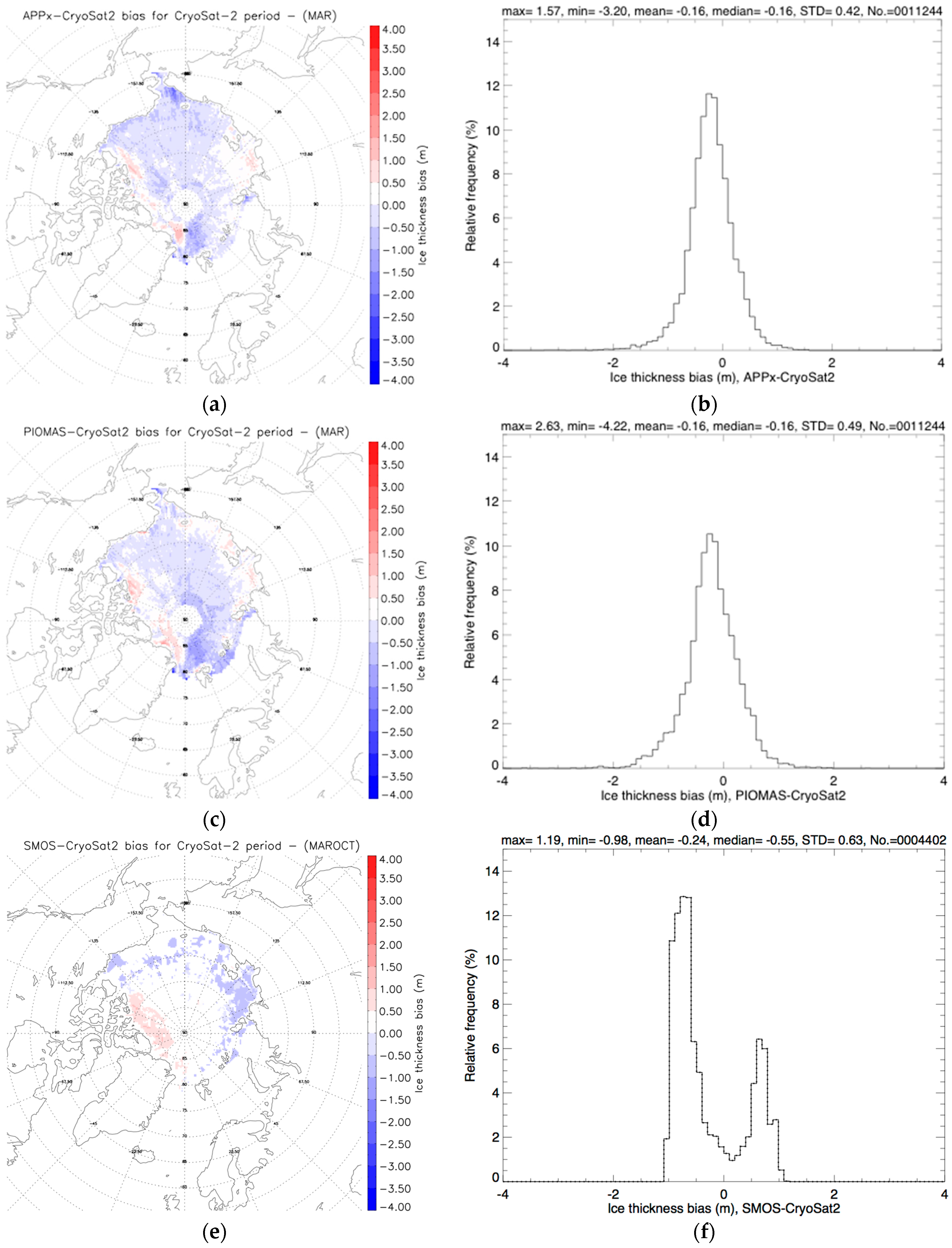
Overall, APP-x best matches CryoSat-2 thicknesses in both Winter and Autumn periods, followed by PIOMAS and SMOS (
Figure 5) in terms of the bias. The biases between APP-x and CryoSat-2 for Winter, Autumn, and combined periods are −0.16 m (−7%), −0.24 m (−18%), and −0.19 m (−10%), respectively, indicating an overall underestimate of sea ice thickness by APP-x relative to CryoSat-2 (
Table 3). Along the north coast of Greenland and the Canadian Archipelago, APP-x ice is thicker than CryoSat-2 (
Figure 5).
The comparison between PIOMAS and CryoSat-2 is very similar to the comparison between APP-x and CryoSat-2. The biases between PIOMAS and CryoSat-2 for Winter, Autumn, and combined periods are −0.16 m (−7%), −0.34 m (−26%), and −0.22 m (−11%), respectively, indicating a substantial sea ice thickness underestimation by PIOMAS as compared to CryoSat-2.
The comparison between SMOS and CryoSat-2 is only done for CryoSat-2 ice thicknesses less than 1 m, given the inherent limitation of the SMOS retrieval. The thin ice biases for Winter, Autumn, and combined periods are 0.13 m (14%), −0.24 m (−30%), and −0.23 m (−28%), respectively. The small correlation coefficients for all the datasets, especially in October, indicate relatively poor agreement over the entire area.
4.3. IceBridge Period
IceBridge sea ice thickness data are available from 2009. For the maximum data overlap between the six datasets, monthly means for March and April, 2011–2013, were used. During this period APP-x, CryoSat-2, SMOS, and PIOMAS are available; ICESat is not.
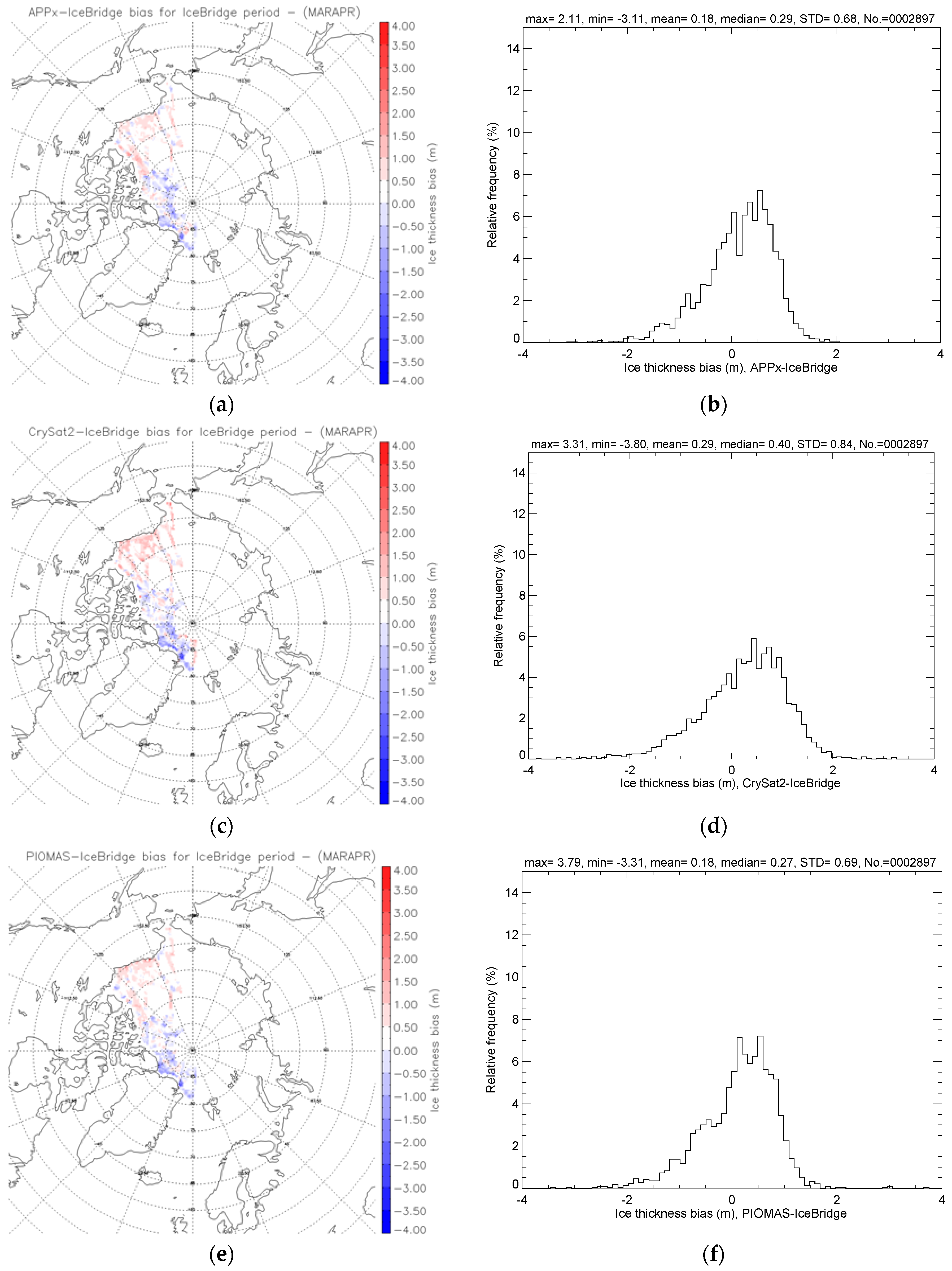
IceBridge campaigns were focused on the western Arctic Ocean, mainly covering the Canadian Archipelago, Canada Basin, and Beaufort Sea (
Figure 6). Overall the APP-x, CryoSat-2, and PIOMAS thicknesses are similar to the IceBridge measurements, with the best spatial agreement for APP-x and PIOMAS with IceBridge. In comparisons of APP-x, CryoSat-2, and PIOMAS with IceBridge, the biases are generally positive. Negative biases are seen in April, but there are significantly fewer pixels (292) than in March (4819). The biases for APP-x, PIOMAS, and CryoSat-2 relative to IceBridge thicknesses are 0.18 m (7%), 0.18 m (7%), and 0.29 m (12%), respectively, for March–April over 2011–2013 (
Table 4). The correlations between APP-x and IceBridge and PIOMAS and IceBridge are relatively high (0.6–0.7), indicating general agreement between the three datasets. As seen in
Figure 6, APP-x, CryoSat-2, and PIOMAS tend to overestimate thicknesses for the thin ice area around the Beaufort Sea, and underestimate the thick ice area around northern Greenland and the Canadian Archipelago.
Similarities and differences for thin ice estimation, defined as ice thicknesses 1 m or less from IceBridge, were examined. As shown in
Table 5, all four datasets (APP-x, PIOMAS, CryoSat-2, and SMOS) have positive biases, indicating overestimates of thin ice relative to IceBridge, with the smallest overall bias of 0.26 m (34%) between SMOS and IceBridge. However, because there were few data available for thin ice from IceBridge in March and no thin ice data at all in April, the thin ice statistics are not statistically significant and this should not be considered as a robust analysis.
5. Discussion
Sea ice thickness can be estimated as a bulk average quantity at instrument specified resolutions from space using laser and radar altimeters to measure ice elevation, visible and infrared data to model the ice thickness that balances the surface energy budget, and passive microwave data with an emissivity model to estimate thin ice. Altimeter approaches may be the most accurate but they do not currently provide long-term, spatially complete data for climate studies. Of course, Cryosat-2, the near-future ICESat-2, and ESA’s Sentinel-3A have the potential to provide many years of data in the future. The use of visible/infrared instruments for estimating ice thickness is the least direct approach but covers the longest time period, can be continued indefinitely, and provides broad coverage on a daily basis. SMOS estimates of ice thickness are useful for studies of relatively thin ice (less than 1 m at most). Submarine data have provided multi-decadal ice thickness estimates as well, though limited in spatial coverage.
This paper presented an inter-comparison of current satellite-based sea ice thickness products. Each of the products examined have been presented in the literature, and each has a stated uncertainty [
8,
9,
10,
11,
13,
15]. The uncertainty in sea ice thickness estimates from space is, however, difficult to determine given the lack of in situ thickness measurements. The accuracy of each product is not further evaluated here. Instead, the differences between the products are quantitatively assessed in order to provide insight into the strengths and weaknesses of each.
The primary factor affecting ice thickness estimates for all datasets is the depth of snow on the ice [
8,
9,
10,
11,
13], except for the IceBridge retrievals that utilize the snow radar for snow depth estimates. Even so, the IceBridge data may have nontrivial biases [
24]. The APP-x, CryoSat-2, and SMOS methods all used a snow climatology from [
32] to estimate snow depth on ice. ICESat used its own daily snow depth field for a snow depth adjustment [
8], and PIOMAS also estimates 12-category snow depth distribution based on a modeling method [
16]. Other factors that affect the OTIM energy budget approach and the PIOMAS model include surface skin and air temperature, surface albedo, cloud cover, and dynamics [
31]. The sensitivity of OTIM retrievals to uncertainties in its input parameters is examined in [
13], where it was found that snow depth is the main source of uncertainty.
6. Conclusions
Results show that ICESat ice thickness are greater than APP-x and PIOMAS overall, particularly along the north coast of Greenland and the Canadian Archipelago, although ICESat sea ice is thinner than APP-x and PIOMAS in the thinner ice areas of the Chukchi, Laptev, and Beaufort Seas. APP-x and PIOMAS show less spatial variation than ICESat. The overall differences between APP-x and PIOMAS with ICESat are −22% and −15% (−0.48 m and −0.31 m), respectively.
APP-x ice thickness best matches with CryoSat-2. The mean differences between APP-x and CryoSat-2 for Winter, Autumn, and combined periods are −7%, −18%, and −10% (−0.16 m, −0.24 m, and −0.19 m), respectively, indicating an overall underestimate of sea ice thickness by APP-x relative to CryoSat-2. When only sea ice thicknesses 1 m and less from CryoSat-2 are considered for comparison, the overall bias between SMOS and CryoSat-2 is -28% (−0.23 m).
The mean differences for APP-x, PIOMAS, and CryoSat-2 relative to IceBridge thicknesses are 7%, 7%, and 12% (0.18 m, 0.18 m, and 0.29 m), respectively. APP-x, CryoSat-2, and PIOMAS tend to overestimate thicknesses for thin ice in the Beaufort Sea area, and underestimate the thick ice area around the north coast of Greenland and Canadian Archipelago relative to IceBridge.
This inter-comparison study has illustrated that there are broad similarities between the various satellite-based ice thickness products, but there are also important differences. APP-x tends to underestimate thick ice, which is not unexpected given that the energy budget approach is less sensitive to changes in the forcing variables for thick ice. In contrast, APP-x and CryoSat-2 methods tend to overestimate thin ice. The altimeter-based approaches are more direct measurements than APP-x, and in theory are more accurate as they are not sensitive to all the factors that affect the energy budget. Nevertheless, the APP-x ice thickness product is useful in that it provides ice thickness estimates beginning in 1982 covering the entire Arctic and Antarctic on a daily basis. While it is important to illustrate the similarities and differences between the various satellite-derived ice thickness products, the next step in evaluating their value is to assess their impact on numerical weather and climate prediction models.
Acknowledgments
This work was supported by the JPSS Program Office, the GOES-R Program Office, the National Science Foundation (ARC-1023371), and the NASA Cryosphere Program (NNX15AG68G). We thank the Alfred Wegener Institute/Helmholtz Centre for Polar and Marine Research and the European Space Agency for making the Cryosat-2 ice thickness product available to the scientific community, the University of Hamburg for the SMOS ice thicknesses, and the National Snow and Ice Data Center and NASA for the IceBridge data. The views, opinions, and findings contained in this report are those of the author(s) and should not be construed as an official National Oceanic and Atmospheric Administration or U.S. Government position, policy, or decision.
Author Contributions
Xuanji Wang designed and applied the OTIM ice thickness algorithm, collected most of the data, performed the analyses, and drafted the manuscript. Jeff Key provided guidance on the study and made substantial contributions to the manuscript. Ron Kwok developed and provided the ICESat ice thickness product. Jinlun Zhang developed and provided the PIOMAS product. Kwok and Zhang also contributed to the manuscript.
Conflicts of Interest
The authors declare no conflict of interest.
Abbreviations
The following abbreviations are used in this manuscript:
| AVHRR | Advanced Very High Resolution Radiometer |
| APP-x | AVHRR Polar Pathfinder-eXtended dataset |
| ICESat | Ice, Cloud, and land Elevation Satellite |
| OTIM | One-dimensional Thermodynamic Ice Model |
| PIOMAS | Pan-Arctic Ice Ocean Modeling and Assimilation System |
| SMOS | ESA’s Soil Moisture and Ocean Salinity mission |
References
- Rind, D.; Healy, R.; Parkinson, C.; Martinson, D.G. The role of sea ice in 2 × CO2 climate model sensitivity. Part I: The total influence of sea ice thickness and extent. J. Clim. 1995, 8, 449–463. [Google Scholar] [CrossRef]
- Randall, D.; Curry, J.; Battisti, D.; Flato, G.; Grumbine, R.; Hakkinen, S.; Martinson, D.; Preller, R.; Walsh, J.; Weatherly, J. Status and outlook for large-scale modeling of atmosphere-ice-ocean interactions in the Arctic. Bull. Am. Meteorol. Soc. 1998, 79, 197–219. [Google Scholar] [CrossRef]
- Intergovernmental Panel on Climate Change (IPCC). Climate Change 2001: The Scientific Basis; IPCC Third Assessment Report; Houghton, J.T., Ding, Y., Griggs, D.J., Noguer, M., van der Linden, P.J., Dai, X., Eds.; Cambridge University Press: Cambridge, UK, 2001. [Google Scholar]
- Curry, J.A.; Rossow, W.B.; Randall, D.; Schramm, J.L. Overview of Arctic cloud and radiative characteristics. J. Clim. 1996, 9, 1731–1764. [Google Scholar] [CrossRef]
- Curry, J.A.; Schramm, J.L.; Alam, A.; Reeder, R.; Arbetter, T.E.; Guest, P. Evaluation of data sets used to force sea ice models in the Arctic Ocean. J. Geophys. Res. 2002, 107, C10. [Google Scholar] [CrossRef]
- Integrated Global Observing Strategy (IGOS). Integrated Global Observing Strategy Cryosphere Theme Report—For the Monitoring of our Environment from Space and from Earth; WMO/TD-No. 1405; World Meteorological Organization: Geneva, Switzerland, 2007. [Google Scholar]
- Kwok, R.; Cunningham, G.F.; Wensnahan, M.; Rigor, I.; Zwally, H.J.; Yi, D. Thinning and volume loss of Arctic sea ice: 2003–2008. J. Geophys. Res. 2009, 114. [Google Scholar] [CrossRef]
- Kwok, R.; Cunningham, G.F. ICESat over Arctic sea ice: Estimation of snow depth and ice thickness. J. Geophys. Res. 2008, 113, C08010. [Google Scholar] [CrossRef]
- Kurtz, N.T.; Farrell, S.L.; Studinger, M.; Galin, N.; Harbeck, J.P.; Lindsay, R.; Onana, V.D.; Panzer, B.; Sonntag, J.G. Sea ice thickness, freeboard, and snow depth products from Operation IceBridge airborne data. Cryosphere 2013, 7, 1035–1056. [Google Scholar] [CrossRef]
- Laxon, S.W.; Giles, K.A.; Ridout, A.L.; Wingham, D.J.; Willatt, R.; Cullen, R.; Kwok, R.; Schweiger, A.; Zhang, J.; Haas, C.; et al. CryoSat-2 estimates of Arctic sea ice thickness and volume. Geophys. Res. Lett. 2013, 40, 732–737. [Google Scholar] [CrossRef]
- Tian-Kunze, X.; Kaleschke, L.; Maaß, N.; Mäkynen, M.; Serra, N.; Drusch, M.; Krumpen, T. SMOS-derived thin sea ice thickness: Algorithm baseline, product specifications and initial verification. Cryosphere 2014, 8, 997–1018. [Google Scholar] [CrossRef] [Green Version]
- Lindsay, R.; Schweiger, A. Arctic sea ice thickness loss determined using subsurface, aircraft, and satellite observations. Cryosphere 2015, 9, 269–283. [Google Scholar] [CrossRef]
- Wang, X.; Key, J.R.; Liu, Y. A thermodynamic model for estimating sea and lake ice thickness with optical satellite data. J. Geophys. Res. 2010, 115, C12035. [Google Scholar] [CrossRef]
- Key, J.; Wang, X.; Liu, Y.; Dworak, R.; Letterly, A. The AVHRR polar pathfinder climate data records. Remote Sens. 2016. [Google Scholar] [CrossRef]
- Huntemann, M.; Heygster, G.; Kaleschke, L.; Krumpen, T.; Mäkynen, M.; Drusch, M. Empirical sea ice thickness retrieval during the freeze up period from SMOS high incident angle observations. Cryosphere 2014, 8, 439–451. [Google Scholar] [CrossRef] [Green Version]
- Zhang, J.; Rothrock, D.A. Modeling global sea ice with a thickness and enthalpy distribution model in generalized curvilinear coordinates. Mon. Weather Rev. 2003, 131, 845–861. [Google Scholar] [CrossRef]
- Wang, X.; Key, J.R. Arctic surface, cloud, and radiation properties based on the AVHRR polar pathfinder data set. Part I: Spatial and temporal characteristics. J. Clim. 2005, 18, 2558–2574. [Google Scholar] [CrossRef]
- National Snow and Ice Data Center (NSIDC). Sea Ice Concentration Data. Available online: http://nsidc.org/data/nsidc-0051.html (accessed on 12 July 2015).
- Kwok, R.; Cunningham, G.F.; Zwally, H.J.; Yi, D. Ice, Cloud, and land Elevation Satellite (ICESat) over Arctic sea ice: Retrieval of freeboard. J. Geophys. Res. 2007, 112, C12013. [Google Scholar] [CrossRef]
- Center for Polar Observation and Modelling (CPOM). CryoSat-2 Ice Thickness Estimates, Including the Quick-Look Datasets Provided to the Community. Available online: http://www.cpom.ucl.ac.uk/csopr/seaice.html (accessed on 24 September 2015).
- Kurtz, N.T.; Galin, N.; Studinger, M. An improved CryoSat-2 sea ice freeboard retrieval algorithm through the use of waveform fitting. Cryosphere 2014, 8, 1217–1237. [Google Scholar] [CrossRef] [Green Version]
- Alfred Wegener Institute (AWI). CryoSat-2 Sea Ice Thickness Data. Available online: http://mep-datasrv1.awi.de/gallery/index_new.php?lang=en_US&active-tab=welcome (accessed on 23 September 2015).
- Integrated Climate Data Center (ICDC). SMOS daily Arctic Sea Ice Thickness Data. Available online: http://icdc.zmaw.de/1/daten/cryosphere/l3c-smos-sit.html (accessed on 29 September 2015).
- Kwok, R.; Haas, C. Effects of radar side-lobes on snow depth retrievals from Operation IceBridge. J. Glaciol. 2015, 61, 576–584. [Google Scholar] [CrossRef]
- National Snow and Ice Data Center (NSIDC). IceBridge Sea Ice Thickness Data. Available online: http://nsidc.org/data/docs/daac/icebridge/idcsi4/index.html (accessed on 3 September 2015).
- Kurtz, N.; Studinger, M.S.; Harbeck, J.; Onana, V.; Yi, D. IceBridge L4 Sea Ice Freeboard, Snow Depth, and Thickness; NASA DAAC at the National Snow and Ice Data Center: Boulder, CO, USA, 2015. [Google Scholar]
- Doble, M.J.; Skourup, H.; Wadhams, P.; Geiger, C.A. The relation between Arctic sea ice surface elevation and draft: A case study using coincident AUV sonar and airborne scanning laser. J. Geophys. Res. 2011, 116, C00E03. [Google Scholar] [CrossRef]
- Thorndike, A.S.; Rothrock, D.A.; Maykut, G.A.; Colony, R. The thickness distribution of sea ice. J. Geophys. Res. 1975, 80, 4501–4513. [Google Scholar] [CrossRef]
- Zhang, J.; Rothrock, D.A. A thickness and enthalpy distribution sea-ice model. J. Phys. Oceanogr. 2001, 31, 2986–3001. [Google Scholar] [CrossRef]
- Flato, G.M.; Hinler, W.D., III. Ridging and strength in modeling the thickness distribution of Arctic sea ice. J. Geophys. Res. 1995, 100, 18611–18626. [Google Scholar] [CrossRef]
- Schweiger, A.; Lindsay, R.; Zhang, J.; Steele, M.; Stern, H. Uncertainty in modeled arctic sea ice volume. J. Geophys. Res. 2011, 116, C00D06. [Google Scholar] [CrossRef]
- Warren, S.G.; Rigor, I.G.; Untersteiner, N.; Radionov, V.F.; Bryazgin, N.N.; Aleksandrov, Y.I.; Colony, R. Snow depth on Arctic sea ice. J. Clim. 1999, 12, 1814–1829. [Google Scholar] [CrossRef]
Figure 1.
The time coverage of the six sea ice thickness datasets as used in this study. All but ICESat continue to the present day. The dataset overlap periods are shaded. An Arctic map with analysis regions is also shown.
Figure 1.
The time coverage of the six sea ice thickness datasets as used in this study. All but ICESat continue to the present day. The dataset overlap periods are shaded. An Arctic map with analysis regions is also shown.
Figure 2.
Sea ice thickness from APP-x (a); CryoSat-2 (b); SMOS (c); PIOMAS (d); IceBridge (e); and ICESat (f). These are the monthly mean results for March 2012, except for ICESat sea ice thickness, which is a 34-day average from 2 February to 31 March 2008.
Figure 2.
Sea ice thickness from APP-x (a); CryoSat-2 (b); SMOS (c); PIOMAS (d); IceBridge (e); and ICESat (f). These are the monthly mean results for March 2012, except for ICESat sea ice thickness, which is a 34-day average from 2 February to 31 March 2008.
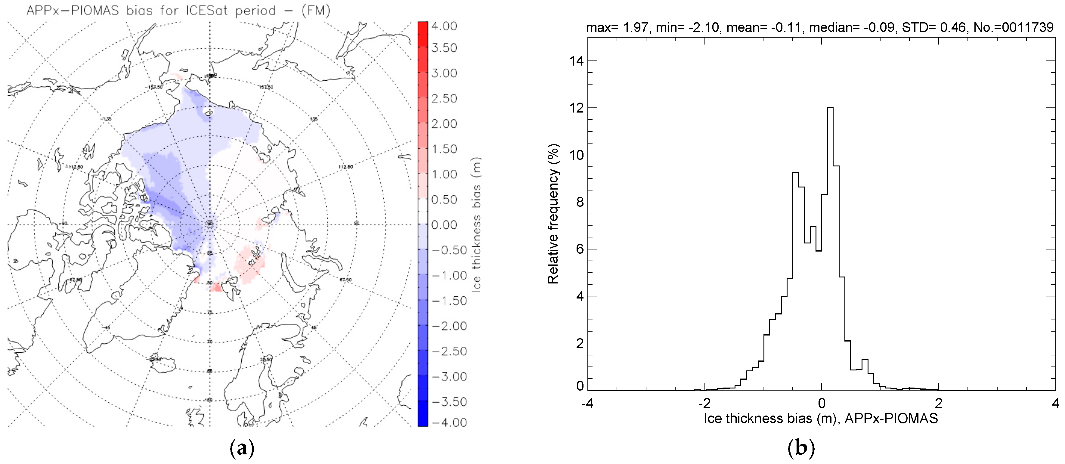
Figure 3.
(a–d) Comparison of sea ice thickness from APP-x and PIOMAS relative to ICESat sea ice thickness for the winter period (FM) over 2003–2008. The bias images for APP-x in (a) and PIOMAS in (c) are shown on the left; the bias histograms for APP-x in (b) and PIOMAS in (d) are shown on the right.
Figure 4.
Comparisons in sea ice thickness between APP-x and PIOMAS for the Winter period (FM) over 2003–2008. The bias image in (a) is shown on the left, and the bias histogram in (b) is shown on the right. The correlation coefficients between APP-x and PIOMAS are 0.67, 0.69, and 0.51 for the periods of FMON, FM, and ON, respectively. (a) Bias image between APP-x and PIOMAS; (b) Bias histogram between APP-x and PIOMAS.
Figure 5.
(a–f) Comparisons in sea ice thickness from APP-x, PIOMAS, and SMOS in terms of CryoSat-2 sea ice thickness for the Winter period (MAR), 2011–2013. The bias images for APP-x in (a); PIOMAS in (c); and SMOS in (e) are shown on the left, and the bias histograms for APP-x in (b); PIOMAS in (d); and SMOS in (f) are shown on the right. The SMOS results are only for CryoSat-2 thicknesses of 1 m and less.
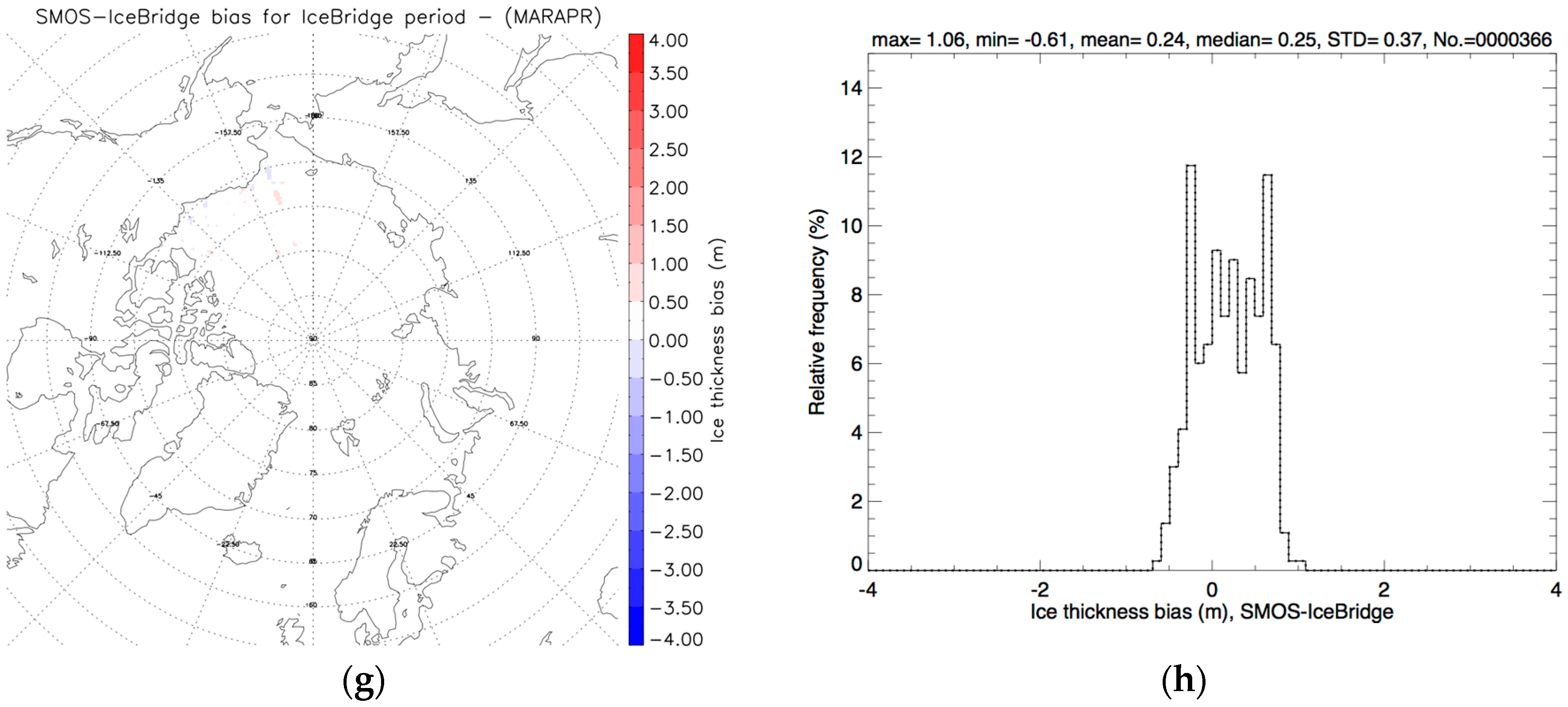
Figure 6.
(a–h) Comparisons in sea ice thickness from APP-x, CryoSat-2, PIOMAS, and SMOS in terms of IceBridge sea ice thickness for March (MAR) and April (APR), 2011–2013. The bias images for APP-x in (a); CryoSat-2 in (c); PIOMAS in (e); and SMOS in (g) are shown on the left, and the bias histograms for APP-x in (b); CryoSat-2 in (d); PIOMAS in (f); and SMOS in (h) are shown on the right. The SMOS results are only for IceBridge thicknesses of 1 m and less.
Table 1.
Characteristics of each satellite or aircraft ice thickness product.
Table 1.
Characteristics of each satellite or aircraft ice thickness product.
| Product | APP-x | ICESat | Cryosat-2 | IceBridge | SMOS |
|---|
| Time Period | 1982-present | 2003–2008 | 2011–present | 2009–present | 2010–present |
| Days for Full Arctic Coverage | Daily | 91 days | 28 days | None | Daily |
| Spatial resolution | 1–25 km | 25 km | 25 km | 40–300 m | 25 km |
| Clear or all sky | All | Clear | All | Clear | All |
| Direct measurement of | Surface temperature, albedo, clouds | Surface elevation | Near-surface elevation | Surface elevation and snow depth | Brightness temperatures |
| Measurement range | 0~5 m | unlimited | unlimited | unlimited | 0~0.5 m |
| Accuracy | 0.20 m | 0.14 | 0.10 m | 0.18 m | 0.10 m |
| Uncertainty (RMS) | 0.54 m | 0.63 | 0.62 m | 0.78 m | 0.16 m |
Table 2.
Descriptive statistics for ice thickness in the three datasets (top half) and their differences and correlation with ICESat thickness (bottom half) in the three ICESat periods (meters). FM is February-March; ON is October-November; FMON is February, March, October, and November. The number in parentheses beneath the period name is the total number of pixels used for the comparison in that period. P-values are given in parentheses beneath the correlation coefficients.
| Period | Statistics | APP-x | PIOMAS | ICESat |
|---|
| FM (55581) | Mean | 2.14 | 2.26 | 2.30 |
| STD | 0.35 | 0.71 | 0.99 |
| Median | 2.09 | 2.14 | 2.01 |
| Mode | 2.11 | 2.11 | 1.75 |
| Skewness | 1.68 | 1.07 | 1.44 |
| ON (55740) | Mean | 1.10 | 1.32 | 1.91 |
| STD | 0.15 | 0.86 | 1.21 |
| Median | 1.12 | 1.39 | 1.60 |
| Mode | 1.19 | 0.02 | none |
| Skewness | −0.71 | 0.39 | 1.05 |
| FMON (111321) | Mean | 1.62 | 1.79 | 2.10 |
| STD | 0.58 | 0.92 | 1.12 |
| Median | 1.51 | 1.84 | 1.86 |
| Mode | 1.19 | 1.93 | none |
| Skewness | 0.56 | 0.19 | 1.06 |
| Bias statistics and dataset correlation with ICESat |
| FM | mean | −0.16 | −0.05 | - |
| STD | 0.63 | 0.54 | - |
| Correlation | 0.71
(<0.001) | 0.68
(<0.001) | - |
| Median | 0.06 | 0.08 | - |
| Mode | none | none | - |
| Skewness | −1.13 | −0.94 | - |
| ON | mean | −0.81 | −0.59 | - |
| STD | 1.16 | 0.80 | - |
| Correlation | 0.42
(<0.001) | 0.75
(<0.001) | |
| Median | −0.54 | −0.52 | - |
| Mode | none | 0.02 | - |
| Skewness | −1.01 | −1.13 | - |
| FMON | mean | −0.48 | −0.31 | - |
| STD | 1.04 | 0.81 | - |
| Correlation | 0.40
(<0.001) | 0.69
(<0.001) | |
| Median | −0.24 | −0.18 | - |
| Mode | none | none | - |
| Skewness | −1.25 | −0.94 | - |
Table 3.
Descriptive statistics of ice thickness in the four datasets (top half) and their differences and correlation with CryoSat-2 thickness (bottom half) in the two CryoSat-2 periods (meters). MAR is March; OCT is October; MAROCT is March and October. The number in parentheses beneath the period name is the total number of pixels used for the comparison in that period. P-values are given in parentheses beneath the correlation coefficients.
| Period | Statistics | APP-x | PIOMAS | SMOS * | CryoSat-2 |
|---|
MAR
(33612) | Mean | 2.14 | 2.14 | 1.04 | 2.31 |
| STD | 0.44 | 0.59 | 0.45 | 0.60 |
| Median | 2.06 | 2.05 | 0.94 | 2.25 |
| Mode | 2.08 | 2.07 | 0.60 | 2.32 |
| Skewness | 1.61 | 0.93 | 0.30 | 1.00 |
OCT
(18068) | Mean | 1.05 | 0.96 | 0.58 | 1.30 |
| STD | 0.21 | 0.61 | 0.63 | 0.47 |
| Median | 1.07 | 0.83 | 0.22 | 1.23 |
| Mode | 1.04 | 0.49 | 1.57 | 0.97 |
| Skewness | −0.97 | 0.88 | 0.70 | 1.64 |
MAROCT
(51680) | Mean | 1.76 | 1.73 | 0.59 | 1.95 |
| STD | 0.62 | 0.82 | 0.63 | 0.74 |
| Median | 1.86 | 1.87 | 0.24 | 1.93 |
| Mode | 1.04 | 1.99 | 1.57 | 2.22 |
| Skewness | 0.19 | 0.11 | 0.67 | 0.57 |
| Bias statistics and dataset correlation with CryoSat-2 |
| MAR | mean | −0.16 | −0.16 | 0.13 | - |
| STD | 0.60 | 0.68 | 0.44 | - |
| Correlation | 0.33
(<0.001) | 0.35
(<0.001) | 0.140
(0.108) | - |
| Median | −0.13 | −0.14 | 0.01 | - |
| Mode | 0.00 | 0.00 | 0.68 | - |
| Skewness | −0.85 | −0.53 | 0.28 | - |
| OCT | mean | −0.24 | −0.34 | −0.24 | - |
| STD | 0.51 | 0.71 | 0.65 | - |
| Correlation | 0.04
(<0.001) | 0.14
(<0.001) | −0.04
(0.003) | - |
| Median | −0.20 | −0.42 | −0.55 | - |
| Mode | 0.00 | −0.37 | −0.92 | - |
| Skewness | −1.15 | −0.13 | 0.72 | - |
| MAROCT | mean | −0.19 | −0.22 | −0.23 | - |
| STD | 0.57 | 0.70 | 0.65 | - |
| Correlation | 0.66
(<0.001) | 0.61
(<0.001) | −0.03
(0.050) | - |
| Median | −0.16 | −0.25 | −0.53 | - |
| Mode | 0.00 | 0.00 | −0.92 | - |
| Skewness | −0.90 | −0.39 | 0.69 | - |
Table 4.
Descriptive statistics of the ice thickness (top half) in five datasets and their differences and correlation with IceBridge thickness (bottom half) in the two IceBridge periods (meters). MAR is March; APR is April; MARAPR is March and April. The number in parentheses beneath the period name is the total number of pixels used for the comparison in that period. P-values are given in parentheses beneath the correlation coefficients.
| Period | Statistics | APP-x | PIOMAS | CryoSat-2 | IceBridge |
|---|
MAR
(4819) | Mean | 2.45 | 2.44 | 2.49 | 2.27 |
| STD | 0.56 | 0.55 | 0.60 | 1.03 |
| Median | 2.39 | 2.49 | 2.39 | 2.16 |
| Mode | 2.33 | 2.89 | 2.32 | 1.89 |
| Skewness | 0.44 | 0.04 | 0.92 | 0.70 |
APR
(292) | Mean | 2.94 | 2.80 | 3.23 | 3.38 |
| STD | 0.54 | 0.58 | 1.01 | 1.25 |
| Median | 2.92 | 2.94 | 3.52 | 3.05 |
| Mode | 2.42 | 2.33 | 3.63 | 3.70 |
| Skewness | 0.06 | −0.05 | -0.42 | 0.62 |
MARAPR
(5111) | Mean | 2.47 | 2.46 | 2.53 | 2.33 |
| STD | 0.57 | 0.56 | 0.65 | 1.08 |
| Median | 2.41 | 2.51 | 2.41 | 2.22 |
| Mode | 2.33 | 2.04 | 2.32 | 3.17 |
| Skewness | 0.41 | 0.05 | 0.95 | 0.76 |
| Bias statistics and dataset correlation with IceBridge |
| MAR | mean | 0.18 | 0.18 | 0.23 | - |
| STD | 0.76 | 0.77 | 0.94 | - |
| Correlation | 0.70
(<0.001) | 0.68
(<0.001) | 0.44
(<0.001) | - |
| Median | 0.28 | 0.25 | 0.30 | - |
| Mode | 0.70 | none | none | - |
| Skewness | −0.88 | −0.81 | −0.65 | - |
| APR | mean | −0.44 | −0.58 | −0.13 | - |
| STD | 1.00 | 1.02 | 1.85 | - |
| Correlation | 0.64
(<0.001) | 0.60
(<0.001) | 0.33
(<0.001) | - |
| Median | −0.23 | −0.35 | 0.02 | - |
| Mode | 0.27 | −0.31 | 0.40 | - |
| Skewness | −0.32 | −0.30 | −0.48 | - |
| MARAPR | mean | 0.18 | 0.18 | 0.29 | - |
| STD | 0.68 | 0.69 | 0.84 | - |
| Correlation | 0.70
(<0.001) | 0.68
(<0.001) | 0.40
(<0.001) | - |
| Median | 0.25 | 0.23 | 0.29 | - |
| Mode | none | none | none | - |
| Skewness | −0.88 | −0.85 | −0.79 | - |
Table 5.
Same as
Table 4, but for IceBridge thicknesses of 1 m and less.
Table 5.
Same as Table 4, but for IceBridge thicknesses of 1 m and less.
| Period | Statistics | APP-x | PIOMAS | SMOS | CryoSat-2 | IceBridge |
|---|
MAR
(404) | Mean | 1.88 | 1.78 | 1.02 | 2.12 | 0.76 |
| STD | 0.18 | 0.39 | 0.39 | 0.43 | 0.18 |
| Median | 1.83 | 1.85 | 0.99 | 2.10 | 0.78 |
| Mode | 1.82 | 2.04 | 0.76 | 2.08 | 0.97 |
| Skewness | 1.60 | −0.38 | 0.05 | 2.49 | −0.60 |
APR
(0) | Mean | - | - | - | - | - |
| STD | - | - | - | - | - |
| Median | - | - | - | - | - |
| Mode | - | - | - | - | - |
| Skewness | - | - | - | - | - |
MARAPR
(404) | Mean | 1.88 | 1.78 | 1.02 | 2.12 | 0.76 |
| STD | 0.18 | 0.39 | 0.39 | 0.43 | 0.18 |
| Median | 1.83 | 1.85 | 0.99 | 2.10 | 0.78 |
| Mode | 1.82 | 2.04 | 0.76 | 2.08 | 0.97 |
| Skewness | 1.60 | −0.38 | 0.05 | 2.49 | −0.60 |
| Bias statistics and dataset correlation with IceBridge |
| MAR | mean | 1.12 | 1.02 | 0.26 | 1.36 | - |
| STD | 0.24 | 0.37 | 0.37 | 0.46 | - |
| Correlation | 0.16
(0.002) | 0.32
(<0.001) | 0.36
(<0.001) | 0.024
(0.634) | - |
| Median | 1.10 | 1.08 | 0.26 | 1.34 | - |
| Mode | 1.13 | 1.29 | none | 1.29 | - |
| Skewness | 0.88 | 0.03 | −0.06 | 2.51 | - |
| APR | mean | - | - | - | - | - |
| STD | - | - | - | - | - |
| Correlation | - | - | - | - | - |
| Median | - | - | - | - | - |
| Mode | - | - | - | - | - |
| Skewness | - | - | - | - | - |
| MARAPR | mean | 1.12 | 1.02 | 0.26 | 1.36 | - |
| STD | 0.24 | 0.37 | 0.37 | 0.46 | - |
| Correlation | 0.16
(0.002) | 0.32
(<0.001) | 0.36
(<0.001) | 0.024
(0.634) | - |
| Median | 1.10 | 1.08 | 0.26 | 1.34 | - |
| Mode | 1.13 | 1.29 | none | 1.29 | - |
| Skewness | 0.88 | 0.03 | −0.06 | 2.51 | - |
© 2016 by the authors; licensee MDPI, Basel, Switzerland. This article is an open access article distributed under the terms and conditions of the Creative Commons Attribution (CC-BY) license (http://creativecommons.org/licenses/by/4.0/).


