
Tropical Texture Determination by Proximal Sensing Using a Regional Spectral Library and Its Relationship with Soil Classification

Abstract
:
1. Introduction
2. Materials and Methods
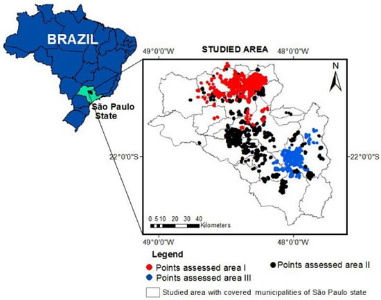
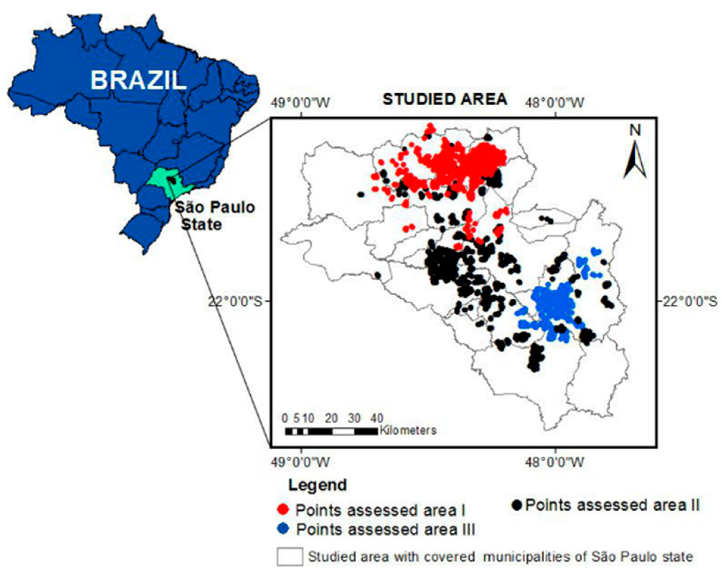
2.1. Location of the Study Site and Sampling Points
2.2. Assessment of Textural Groups of the Soils Studied
2.2.1. Particle Size and Spectroscopic Analyses of Soil Samples
2.2.2. Assessment of Textural Groups
2.2.3. Particle Size Assessment vs. Spectral Data
2.3. Quantitative and Descriptive Spectral Assessment
2.3.1. Assessment of Principal Component Analysis (PCA)
2.3.2. Prediction Models for Soil Attributes
2.3.3. Assessment of Attribute Prediction Model-Descriptive Statistical Analyses
2.3.4. Ternary Diagrams of Textural Classification Ofsoils: Real vs. Espectral Values
2.4. Spectral Soil Classification
3. Results and Discussion
3.1. Assessment of Textural Groups of the Soils Studied
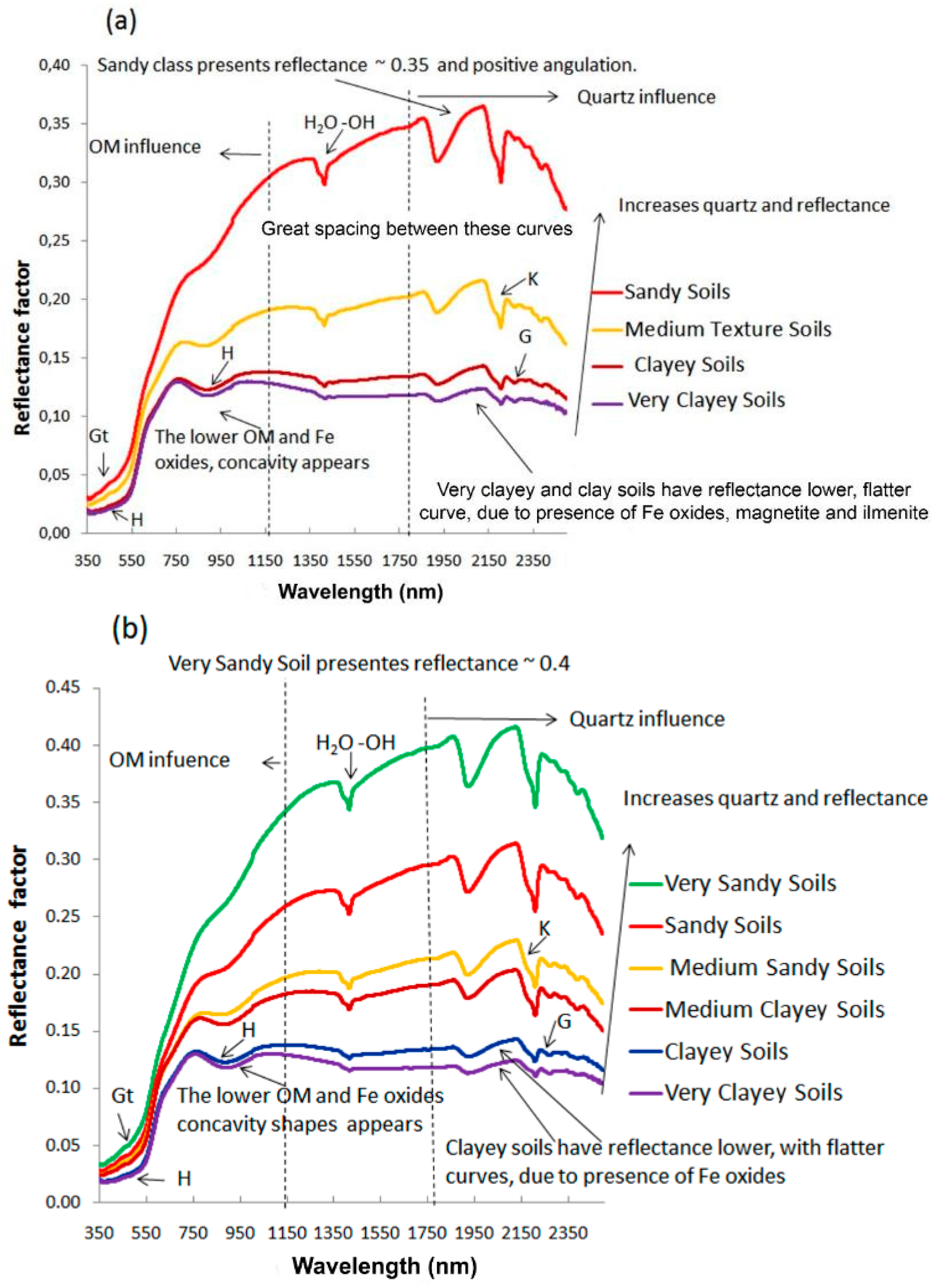
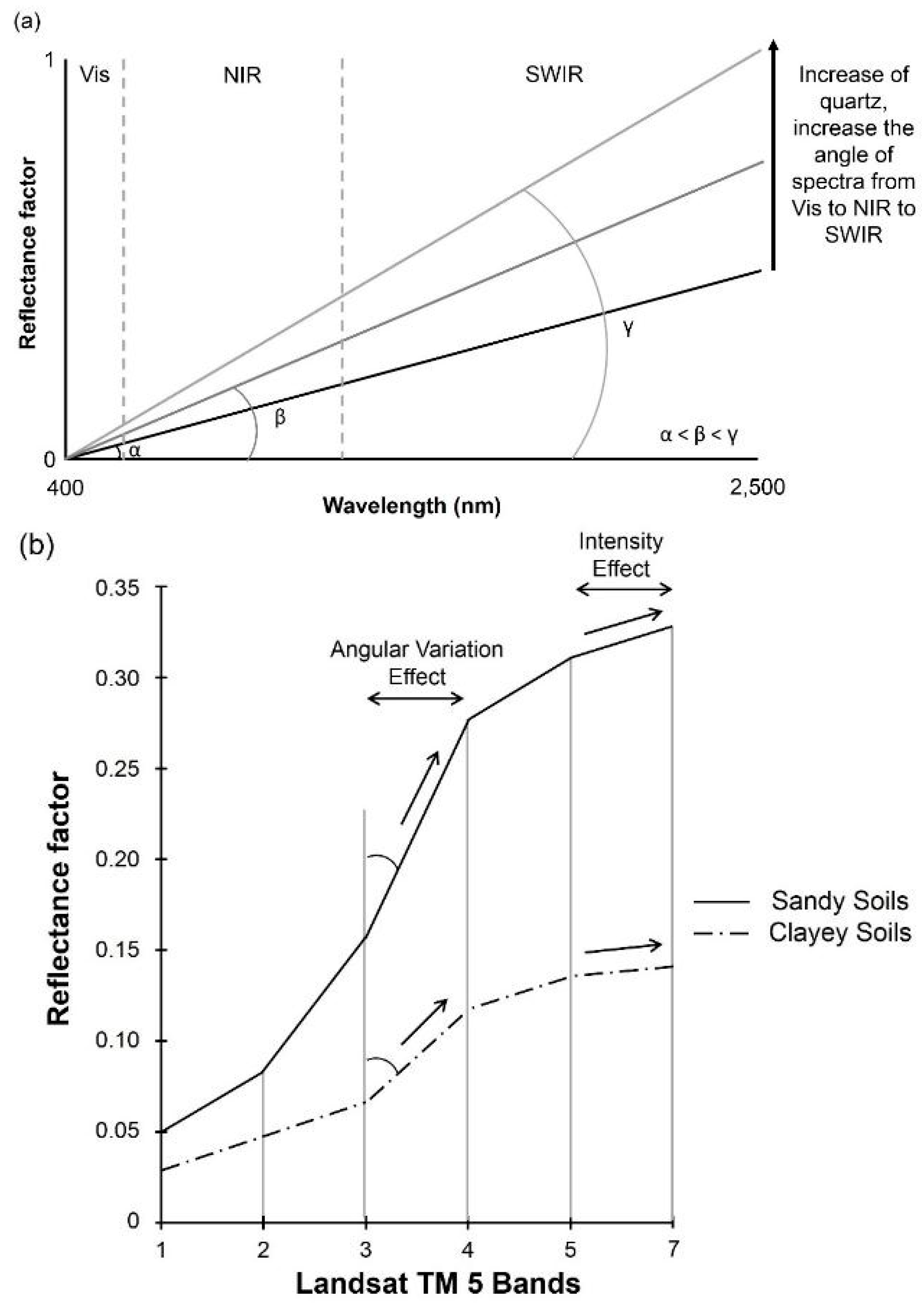
Spectroscopic Analyses of Soil Samples
3.2. Quantitative and Descriptive Spectral Assessment of the Soils Studied
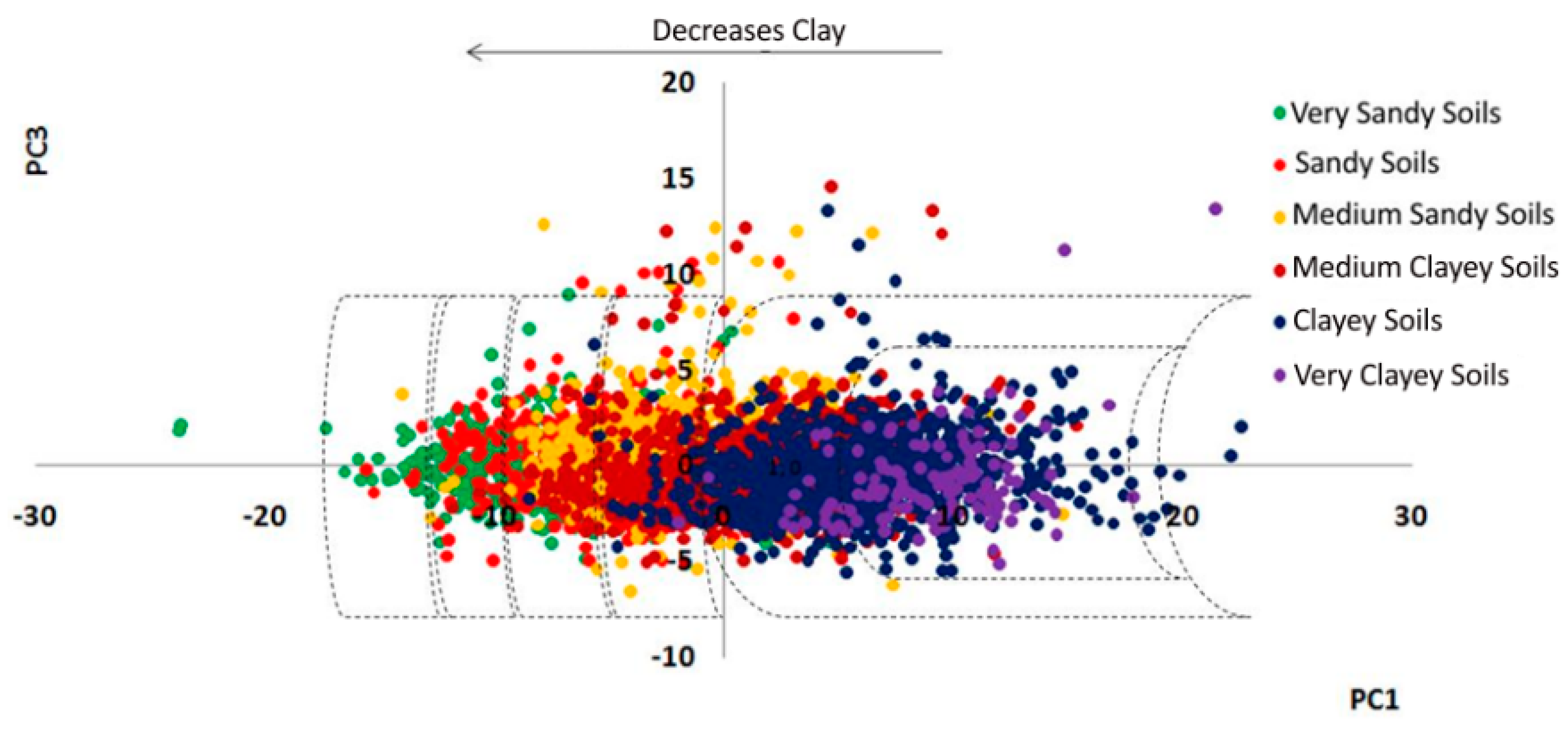
3.2.1. Principal Component Analysis (PCA)
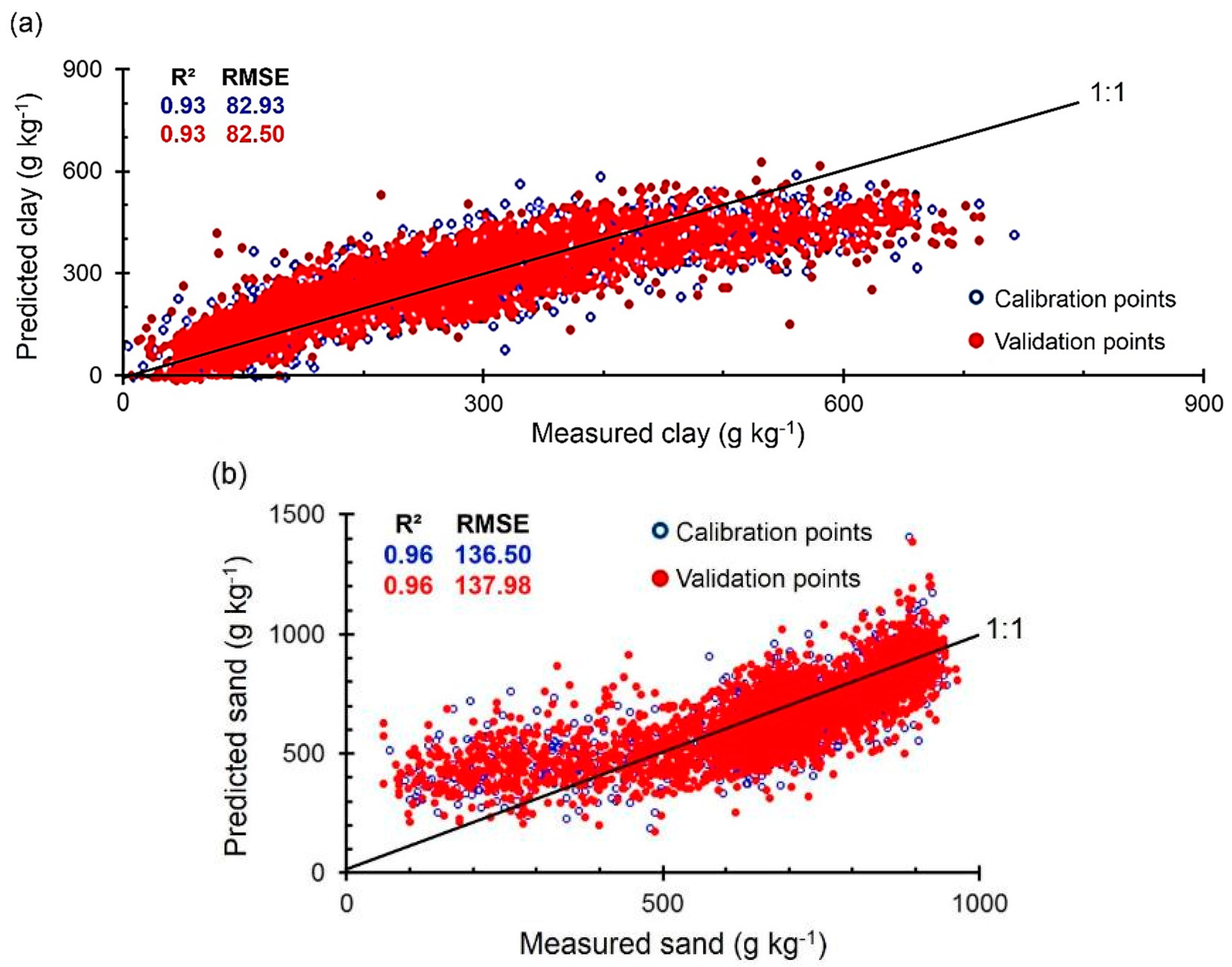
3.2.2. Prediction Models of Soil Attributes
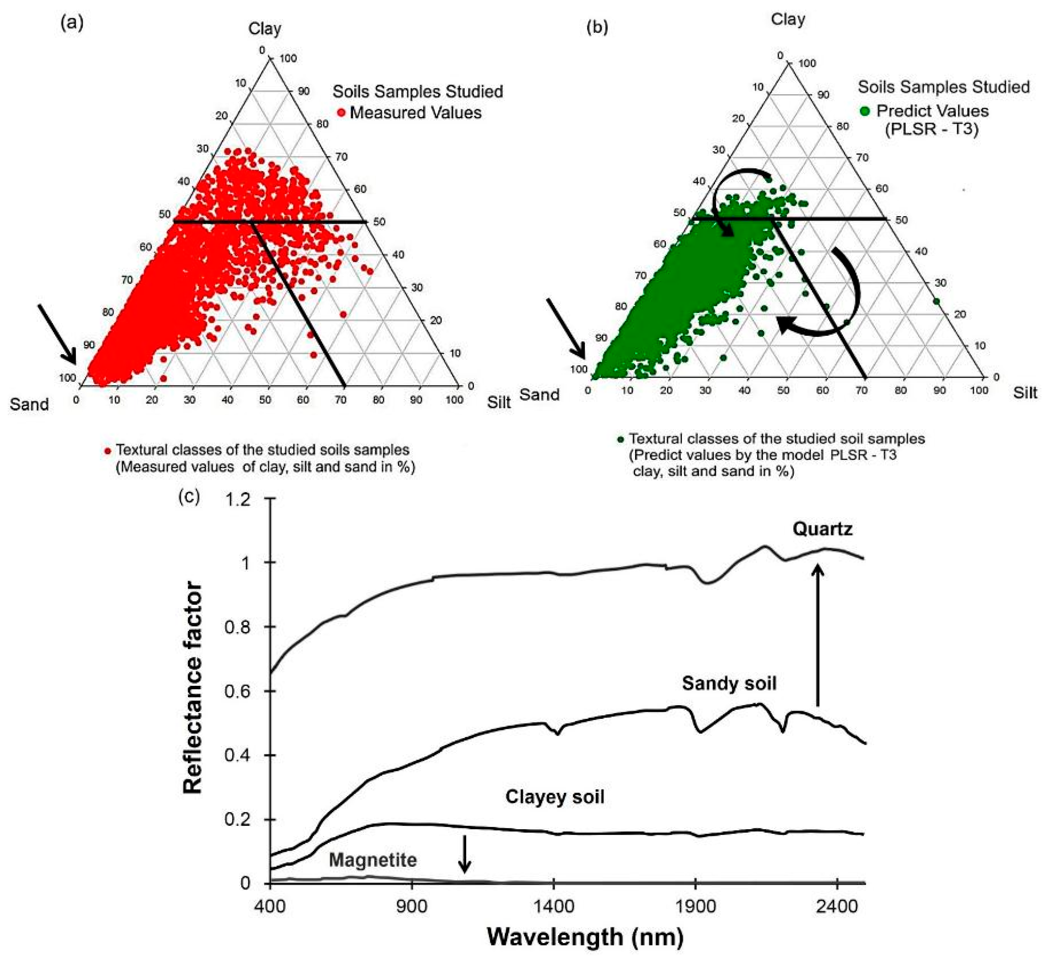
3.2.3. Ternary Diagrams of Textural Classification of Soils: Real vs. Spectral Values
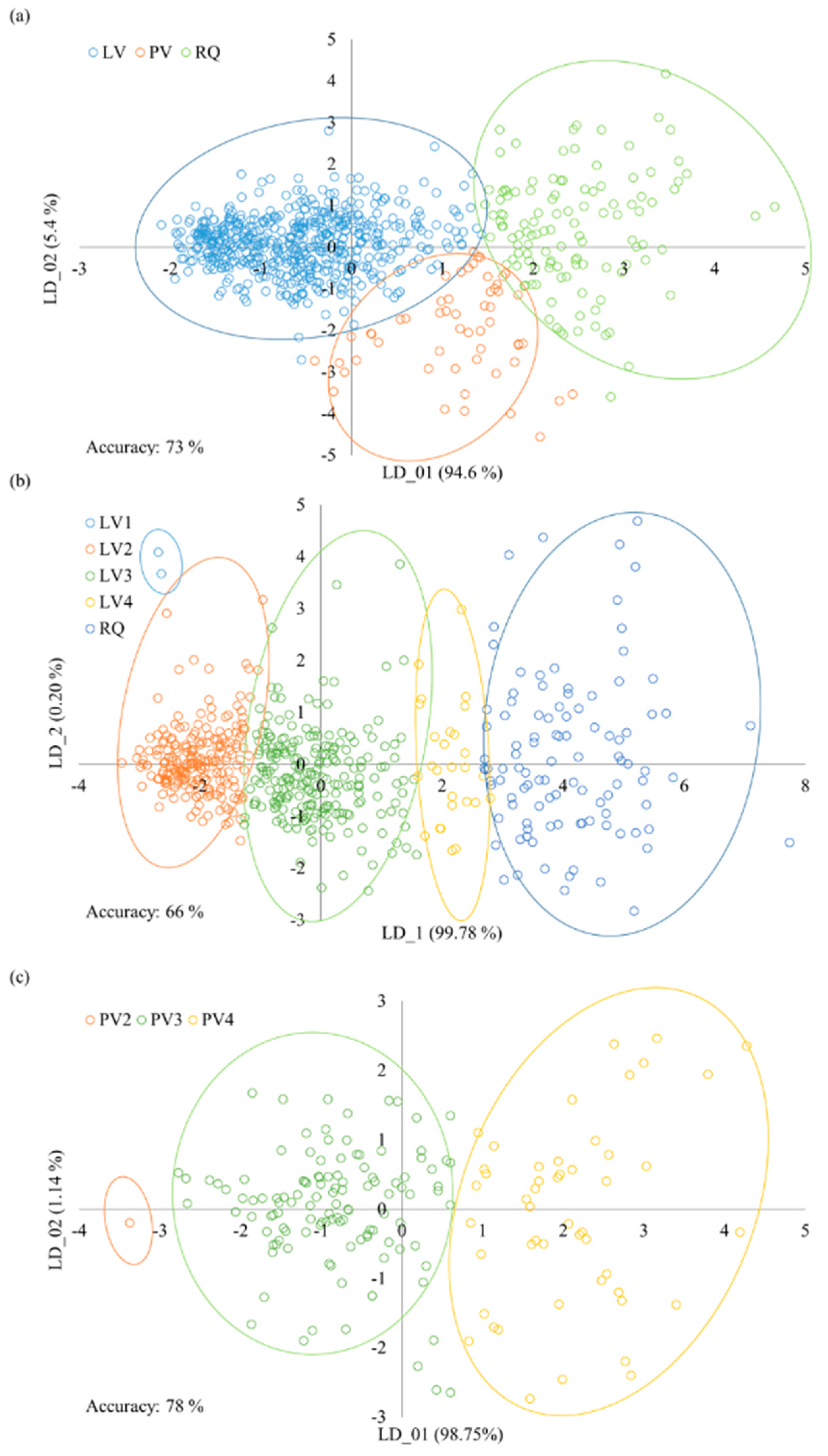
3.4. Soil Spectral Classification by Textural Information
5. Conclusions
Acknowledgments
Author Contributions
Conflicts of Interest
References
- Demattê, J.L.I.; Demattê, J.A.M. Environment productivity as a strategy for sugar cane culture. Inform. Agron. 2009, 127, 10–18. [Google Scholar]
- Mendonça-Santos, M.L.; Santos dos, H.G. The state of the art of Brazilian soil mapping and prospects for digital soil mapping. In Digital Soil Mapping An Introductory Perspective; Lagacherie, P., McBratney, A.B., Voltz, B.T., Eds.; Elsevier: Amsterdam, The Netherlands, 2006; pp. 39–54. [Google Scholar]
- Camargo, M.N.; Klant, E.; Kauffman, J.H. Classificação de solos usada em levantamentos pedológicos no Brasil. Soc. Bras. Ciênc. Solo 1987, 12, 11–13. [Google Scholar]
- Embrapa—Empresa Brasileira de Pesquisa Agropecuária. Sistema Brasileiro de Classificação de Solos, 3rd ed.; Centro Nacional de Pesquisa de Solos, Embrapa: Brasília, Brazil, 2013. [Google Scholar]
- FAO—Food and Agriculture Organization of United Nations. World Reference Base for Soil Resources; FAO/International Soil Reference and Information Centre-ISRIC/International Union of Soil Sciences-IUSS: New York, NY, USA, 2006. [Google Scholar]
- Demattê, J.A.M.; Garcia, G.J. Avaliação de atributos de latossolo bruno e de Terra bruna estruturada da região de Guarapuava, Paraná, por meio de sua energia refletida. Rev. Bras. Ciênc. Solo 1999, 23, 343–355. [Google Scholar] [CrossRef]
- Franceschini, M.H.D.; Demattê, J.A.M.; da Terra, F.S.; Vicente, L.E.; Bartholomeus, H.; Souza Filho, C.R. Prediction of soil properties using imaging spectroscopy: Considering fractional vegetation cover to improve accuracy. Int. J. Appl. Earth Obs. Geoinf. 2015, 38, 358–370. [Google Scholar] [CrossRef]
- Dalmolin, R.S.D.; Gonçalves, C.N.; Klamt, E.; Dick, D.P. Relação entre os constituintes do solo e seu comportamento espectral. Cienc. Rural 2005, 35, 481–489. [Google Scholar] [CrossRef]
- Terra, F.S.; Demattê, J.A.M.; Viscarra-Rossel, R.A. Spectral libraries for quantitative analyses of tropical Brazilian soils: Comparing vis–NIR and mid-IR reflectance data. Geoderma 2015, 255–256, 81–93. [Google Scholar] [CrossRef]
- Shepherd, K.D.; Walsh, M.G. Development of reflectance spectral libraries for characterization of soil properties. Soil Sci. Soc. Am. J. 2002, 66, 988–998. [Google Scholar] [CrossRef]
- Ben-Dor, E. Quantitative remote sensing of soil properties. Adv. Agron. 2002, 75, 173–243. [Google Scholar]
- Dunn, B.W.; Beecher, H.G.; Batten, G.D.; Ciavarella, S. The potential of near-infrared reflectance spectroscopy for soil analysis—A case study from the Riverine Plain of south-eastern Australia. Aust. J. Exp. Agric. 2002, 42, 607–614. [Google Scholar] [CrossRef]
- Viscarra-Rossel, R.A.; Walvoort, D.J.J.; Mcbratney, A.B.; Janik, L.J.; Skjemstad, J.O. Visible, near infrared, mid infrared or combined diffuse reflectance spectroscopy for simultaneous assessment of various soil properties. Geoderma 2006, 131, 59–75. [Google Scholar] [CrossRef]
- Nanni, M.R.; Demattê, J.A.M. Spectral reflectance methodology in comparison to traditional soil analysis. Soil Sci. Soc. Am. J. 2006, 70, 393–407. [Google Scholar] [CrossRef]
- Brown, D.J.; Shepherd, M.G.W.; Walsh, M.G.; Mays, M.D.; Reinsch, T.G. Global soil characterization with VNIR diffuse reflectance spectroscopy. Geoderma 2006, 132, 273–290. [Google Scholar] [CrossRef]
- Maleki, M.R.; Mouazen, A.M.; Ramon, H.; de Baerdemaeker, J. Optimization of soil VIS-NIR sensor-based variable rate application system of soil phosphorus. Soil Tillage Res. 2007, 94, 239–250. [Google Scholar] [CrossRef]
- Mouazen, A.M.; Maleki, M.R.; de Baerdemaeker, J.; Ramon, H. On-line measurement of some selected soil properties using a VIS–NIR sensor. Soil Tillage Res. 2007, 93, 13–27. [Google Scholar] [CrossRef]
- Summers, D.; Lewis, M.; Ostendorf, B.; Chittleborough, D. Visible near-infrared reflectance spectroscopy as a predictive indicator of soil properties. Ecol. Indic. 2009. [Google Scholar] [CrossRef]
- Soriano-Disla, J.M.; Janik, J.; Viscarra-Rossel, R.A.; Macdonald, L.M.; McLaughlin, M.J. The performance of visible, near, and mid-infrared reflectance spectroscopy for prediction of soil physical, chemical, and biological properties. Appl. Spectrosc. Rev. 2014, 49, 139–186. [Google Scholar] [CrossRef]
- Bellinaso, H.; Demattê, J.A.M.; Araújo, S.R. Soil spectral library and its use in soil classification. Rev. Bras. Ciênc. Solo 2010, 34, 861–870. [Google Scholar] [CrossRef] [Green Version]
- Van Reeuwjik, L.P. Procedure for Soil Analysis, 6th ed.; ISRIC: New York, NY, USA, 2002. [Google Scholar]
- Viscarra Rossel, R.A.; Webster, R. Predicting soil properties from the Australian soil visible near infrared spectroscopic database. Eur. J. Soil Sci. 2012, 63, 848–860. [Google Scholar] [CrossRef]
- USDA—United States Department of Agriculture. Rapid Carbon Assessment (RaCA) Methodology; NRCS/USDA: New York, NY, USA, 2013.
- Stevens, A.; Nocita, M.; Toth, G.; Montanarella, L.; van Wesemael, B. Prediction of soil organic carbon at the European scale by visible and near infrared reflectance spectroscopy. PLoS ONE 2013, 8. [Google Scholar] [CrossRef]
- Nocita, M.; Stevens, A.; van Wesemael, B.; Aitkenhead, M.; Bachmann, M.; Barthès, B.; Ben dor, E.; Brown, D.J.; Clairotte, M.; Csorba, A.; et al. Soil spectroscopy: An alternative to wet chemistry for soil monitoring. In Advances in Agronomy; Sparks, D.L., Ed.; Academic Press: New York, NY, USA, 2015; pp. 139–159. [Google Scholar]
- Embrapa—Empresa Brasileira de Pesquisa Agropecuária, Centro Nacional de Pesquisas de Solos. Manual de Métodos de Análise de Solos, 2nd ed.; Embrapa: Rio de Janeiro, Brasil, 1997. [Google Scholar]
- Chicati, M.L.; Nanni, R.; Cézar, E.; Oliveira, R.B.; Demattê, J.A.M. Análise comparativa da determinação da linha dos solos em área de várzea nos níveis orbital e laboratorial. In Proceedings of the XVI Simpósio Brasileiro de Sensoriamento Remoto, Foz do Iguaçu, Brazil, 13–18 April 2013.
- Huete, A.R. Soil influences in remotely sensed vegetation canopy spectra. In Theory and Application of Optical Remote Sensing; Asrar, G., Ed.; Wiley Interscience: New York, NY, USA, 1989; pp. 107–141. [Google Scholar]
- Fukuhara, M.; Hayasiu, S.; Yasuda, Y. Extraction of soil information from vegetated areas. In Proceedings of the Machine Processing of the Remotely Sensed Data, West Lafayette, IN, USA, 27–29 June 1979.
- Demattê, J.A.M. Characterization and discrimination of soils by their reflected electromagnetic energy. Braz. J. Agric. Res. 2002, 37, 1445–1458. [Google Scholar] [CrossRef]
- Demattê, J.A.M.; Bellinaso, H.; Romero, D.J.; Fongaro, C.T. Morphological Interpretation of Reflectance Spectrum (MIRS) using libraries looking towards soil classification. Sci. Agric. 2014, 71, 509–520. [Google Scholar] [CrossRef]
- CAMO A/S. The Unscrambler User’s Guide; CAMO: Trondheim, Norway, 1998. [Google Scholar]
- Wold, H. Systems under Indirect Observation; Elsevier: Amsterdam, The Netherlands, 1982. [Google Scholar]
- Campbell, N.A.; Mulcahy, M.J.; Mcarthur, W.M. Numerical classification of soil profiles on the basis of field morphological properties. J. Soil Res. 1970, 8, 43–58. [Google Scholar] [CrossRef]
- Chang, C.W.; Laird, D.A.; Mausbach, M.J.; Hurburgh Junior, C.R. Near-infrared reflectance spectroscopy—Principal components regression analyses of soil properties. Soil Sci. Soc. Am. J. 2001, 65, 480–490. [Google Scholar] [CrossRef]
- Franceschini, M.H.D.; Demattê, J.A.M.; Sato, M.V.; Vicente, L.E; Grego, C.R. Abordagens semiquantitativa e quantitativa na avaliação da textura do solo por espectroscopia de reflectância bidirecional no VIS-NIR-SWIR. Pesqui. Agropecu. Bras. 2013, 48, 1568–1581. [Google Scholar] [CrossRef]
- Stenberg, B.; Viscarra-Rossel, R.A.; Mouazen, A.M.; Wetterlind, J. Visible and near infrared spectroscopy in soil science. In Advances in Agronomy; Sparks, D.L., Ed.; Academic Press: Burlington, ON, Canada, 2010; pp. 163–215. [Google Scholar]
- Fisher, R. The use of multiple measurements in taxonomic problems. Ann. Hum. Genet. 1936, 7, 179–188. [Google Scholar] [CrossRef]
- R Core Team. R: A Language and Environment for Statistical Computing; The R Foundation for Statistical Computing: Vienna, Austria, 2016. [Google Scholar]
- Almeida, F.F.M.; Barbosa, O. Geologia das Quadrículas de Piracicaba e Rio Claro, Estado de São Paulo; Departamento Nacional de Pesquisa Mineral/Divisão de Geologia Mineral: Rio de Janeiro, Brazil, 1953. [Google Scholar]
- Stoner, E.R.; Baumgardner, M.F. Characteristics variations in reflectance of surface soils. Soil Sci. Soc. Am. J. 1981, 45, 1161–1165. [Google Scholar] [CrossRef]
- Baret, F.; Jacquemound, S.; Hanoq, J.F. The soil line concept in remote sensing. Remote Sens. Environ. 1983, 7, 1–18. [Google Scholar] [CrossRef]
- Nanni, M.R.; Demattê, J.A.M. Quantification and discrimination of soils developed from basalt as evaluated by terrestrial, airborne and orbital sensors (Compact Disc). In Proceedings of the X Simpósio Brasileiro de Sensoriamento Remoto, Foz do Iguaçu, Brazil, 21–26 April 2001.
- Nanni, M.R.; Demattê, J.A.M. Comportamento da linha do solo obtida por espectrorradiometria laboratorial para diferentes classes de solo. Rev. Bras. Ciênc. Solo 2006, 30, 1031–1038. [Google Scholar] [CrossRef]
- Ferraresi, T.M.; da Silva, W.T.L.; Martin-Neto, L.; da Silveira, P.M.; Madari, B.E. Espectroscopia de infravermelho na determinação da textura do solo. Rev. Bras. Ciênc. Solo 2012, 36, 1769–1777. [Google Scholar] [CrossRef]
- Vendrame, P.R.S.; Marchão, R.L.; Brunet, D.; Becquer, T. The potential of NIR spectroscopy to predict soil texture and mineralogy in Cerrado Latosols. Eur. J. Soil Sci. 2012, 63, 743–753. [Google Scholar] [CrossRef]
- Sørensen, L.K.; Dalsgaard, S. Determination of clay and other soil properties by near infrared spectroscopy. Soil Sci. Soc. Am. J. 2005, 69, 159–167. [Google Scholar] [CrossRef]
- Sayes, W.; Mouazen, A.M.; Ramon, H. Potential for onsite and online analysis of pig manure using visible and near infrared reflectance spectroscopy. BIOS Engl. 2005, 91, 393–402. [Google Scholar] [CrossRef]
- Viscarra-Rossel, R.A.; Mcbratney, A.B. Diffuse reflectance spectroscopy as a tool for digital soil mapping. In Digital Soil Mapping with Limited Data; Hartemink, A.E., McBratney, A.B., Mendonça-Santos, L., Eds.; Springer Netherlands: Dordrecht, The Netherlands, 2008; pp. 165–172. [Google Scholar]
- Viscarra-Rossel, R.A.; Behrens, T. Using data mining to model and interpret soil diffuse reflectance spectra. Geoderma 2010, 158, 46–54. [Google Scholar] [CrossRef]
- Williams, P.C. Implementation of near infrared technology. In Near Infrared Technology in the Agricultural and Food Industries; American Association of Cereal Chemists: Eagan, MN, USA, 2001; pp. 145–169. [Google Scholar]
- Lindberg, J.D.; Snyder, D.G. Diffuse reflectance spectra of several clay minerals. Am. Mineral. 1972, 57, 485–493. [Google Scholar]
- Hunt, G.R. Near-infrared (1.3–2.5 µm) spectra of alteration minerals—Potential for use in remote sensing. Geophysics 1979, 44, 1974–1986. [Google Scholar] [CrossRef]
- Ben-Dor, E.; Banin, A. Near-infrared reflectance analysis of carbonate concentration in soils. Appl. Spectrosc. 1990, 44, 1064–1069. [Google Scholar] [CrossRef]
- Viscarra-Rossel, R.A.; Cattle, S.R.; Ortega, A.; Fouad, Y. In situ measurements of soil color, mineral composition and clay content by Vis–NIR spectroscopy. Geoderma 2009, 150, 253–266. [Google Scholar] [CrossRef]
- Cantarella, H.; Quaggio, J.A.; van Raij, B.; Abreu, M.F. Variability of soil analysis of commercial laboratories: Implications for lime and fertilizer recommendations. Commun. Soil Sci. Plant Anal. 2006, 37, 2213–2225. [Google Scholar] [CrossRef]
- Demattê, J.A.M.; Fiorio, P.R.; Araujo, P.R. Variation of routine soil analysis when compared with hyperspectral narrow band sensing method. Remote Sens. 2010, 2, 1998–2016. [Google Scholar] [CrossRef]
- Cezar, E.; Nanni, M.R.; Chicati, M.L.; Souza Júnior, I.G.; Costa, A.C.S. Use of spectral data for estimating the relationship between iron oxides and 2:1 minerals with their respective reflectances. Semin. Ciênc. Agrár. 2013, 34, 1479–1492. [Google Scholar]


| Statistical Parameters | Measured Values (g·kg−1) | Predicted Values (g·kg−1) | ||||
|---|---|---|---|---|---|---|
| Clay | Silt | Sand | Clay | Silt | Sand | |
| Average | 274.49 | 69.86 | 655.65 | 272.06 | 73.12 | 654.82 |
| Standard error | 2.55 | 1.16 | 3.44 | 2.12 | 1.25 | 2.96 |
| Median | 260 | 45 | 691.5 | 274.22 | 75.81 | 645.16 |
| Mode | 280 | 40 | 680 | 341.88 | 146.19 | 1004 |
| Standard deviation | 155.99 | 70.86 | 210.71 | 130.01 | 76.66 | 181.3 |
| Kurtosis | 0.59 | 2.03 | 0.85 | 0.08 | 0.1 | 0.2 |
| Asymmetry | 740 | 592 | 909 | 830.66 | 1059.86 | 1424 |
| Minimum | 5 | 0 | 60 | −189.4 | −301.79 | 0 |
| Maximum | 745 | 504 | 969 | 641.26 | 758.07 | 1424 |
| Coefficient of variation (%) | 56.83 | 101.43 | 32.14 | 47.79 | 104.84 | 27.69 |
© 2016 by the authors; licensee MDPI, Basel, Switzerland. This article is an open access article distributed under the terms and conditions of the Creative Commons Attribution (CC-BY) license (http://creativecommons.org/licenses/by/4.0/).
Share and Cite
Lacerda, M.P.C.; Demattê, J.A.M.; Sato, M.V.; Fongaro, C.T.; Gallo, B.C.; Souza, A.B. Tropical Texture Determination by Proximal Sensing Using a Regional Spectral Library and Its Relationship with Soil Classification. Remote Sens. 2016, 8, 701. https://doi.org/10.3390/rs8090701
Lacerda MPC, Demattê JAM, Sato MV, Fongaro CT, Gallo BC, Souza AB. Tropical Texture Determination by Proximal Sensing Using a Regional Spectral Library and Its Relationship with Soil Classification. Remote Sensing. 2016; 8(9):701. https://doi.org/10.3390/rs8090701
Chicago/Turabian StyleLacerda, Marilusa P. C., José A. M. Demattê, Marcus V. Sato, Caio T. Fongaro, Bruna C. Gallo, and Arnaldo B. Souza. 2016. "Tropical Texture Determination by Proximal Sensing Using a Regional Spectral Library and Its Relationship with Soil Classification" Remote Sensing 8, no. 9: 701. https://doi.org/10.3390/rs8090701