Proximal Sensing and Digital Terrain Models Applied to Digital Soil Mapping and Modeling of Brazilian Latosols (Oxisols)

Abstract

Digital terrain models (DTM) have been used in soil mapping worldwide. When using such models, improved predictions are often attained with the input of extra variables provided by the use of proximal sensors, such as magnetometers and portable X-ray fluorescence scanners (pXRF). This work aimed to evaluate the efficiency of such tools for mapping soil classes and properties in tropical conditions. Soils were classified and sampled at 39 locations in a regular-grid design with a 200-m distance between samples. A pXRF and a magnetometer were used in all samples, and DTM values were obtained for every sampling site. Through visual analysis, boxplots were used to identify the best variables for distinguishing soil classes, which were further mapped using fuzzy logic. The map was then validated in the field. An ordinary least square regression model was used to predict sand and clay contents using DTM, pXRF and the magnetometer as predicting variables. Variables obtained with pXRF showed a greater ability for predicting soil classes (overall accuracy of 78% and 0.67 kappa index), as well as for estimating sand and clay contents than those acquired with DTM and the magnetometer. This study showed that pXRF offers additional variables that are key for mapping soils and predicting soil properties at a detailed scale. This would not be possible using only DTM or magnetic susceptibility.

1. Introduction

The small scale of most soil maps in Brazil is not suitable for land use planning and for defining soil and water conservation practices, which need to be done in more detail, i.e., at the level of watersheds [1], as established by the current legislation in Brazil [2]. The lack of financial support along with the large area of the country and the scarcity of roads are some of the main issues restricting the creation of more detailed soil maps, since they require intensive field work for sampling and classifying soils. In this sense, digital soil mapping and modeling are viewed as an alternative to increase not only soil information [3], but also the accuracy required for detailed soil maps, by the adoption of new tools and techniques to analyze, integrate and visualize soil and environmental datasets [4]. In recent years, extra effort has been put into the creation and use of new covariates that represent soil-forming factors [5,6], which are crucial for achieving adequate accuracy in soil mapping and a better understanding of soil modeling. Thus, the investigation of the main drivers of pedogenesis, as well as their geographic patterns is a key point for a successful mapping and modeling.

The study area of this work comprises the complete soil-landscape variations of Latosols (Oxisols), whose distribution pattern is commonly observed in the surrounding region. Previous studies have pointed out parent material and age as the main drivers of soil differentiation in the region [7,8]. Such studies attempted to define soil-landscape relationships from erosional surfaces and their relationship with parent material, soil classes and properties. One of the main findings of these studies performed by [7,8] was the low predictive power of topography. It is important to emphasize that during those preliminary findings, geographic information systems and digital elevation models were not available. Besides the predominance of Latosols (Oxisols), these studies highlighted important parent material contrasts, including soils derived from gabbro, leucocratic gneiss (predominance of lighter minerals), and mesocratic gneiss (higher contents of darker minerals), exerting strong influence on soil properties. These studies also indicated the importance of having detailed geologic maps in the region, as well as in most areas of Brazil, which might improve soil maps and prediction models. Such findings reveal the need for new techniques that may well improve the tacit models developed by pedologists. By providing new insights on soil-landscape relationships and detailed information on parent material differentiation, such techniques could offer more specific terrain models through remote sensing data and increase the amount of information about soils, thus improving soil mapping and modeling in the area.

One of the most common soil-forming factors used in the predictions of soil classes and properties is topography [4,9,10,11], by analyses of a digital elevation model and its derivatives (digital terrain models (DTMs)), e.g., slope, terrain curvatures, topographical wetness index, aspect, etc. Such maps have been extensively used in recent years, since soils occur in response to water movement throughout the landscape, which is controlled by local relief [11]. Additionally, considering the continuous nature of DTM variation (raster-based distribution), they have been used in soil predictive models for providing spatially-exhaustive auxiliary variables [12,13], although it is commonly known that soils result from a complex interaction of soil-forming factors [14]. In this sense, the use of DTM is considered very useful in environments where topography is strongly related to the processes driving soil formation [11,15].

Despite the fact that DTMs have been used worldwide as adequate predictors of soil properties, recent studies are searching for new tools associated with soil attributes, especially those concerning chemical features. For example, some soil chemical elements or properties could function as tracers or indicators of different parent materials, which, in turn, could be related to soil classes and properties. At last, this information could potentially improve soil mapping and modeling. In this sense, equipment that performs fast analyses in the field and provides a large spectrum of data, such as proximal sensors, has been recently adopted to help soil mapping. Proximal sensing includes proximal or remote in situ and ex situ (field and laboratory) non-invasive or intrusive and mobile or stationary devices [16]. Some examples are magnetometers, which quantify the magnetic susceptibility of different materials, and portable X-ray fluorescence (pXRF) scanners, used to identify and quantify chemical elements and compounds present in soil samples [17].

Magnetic susceptibility is obtained from the ratio of induced magnetization in relation to the intensity of the magnetizing field and is being considered a simple, sensitive, inexpensive and non-destructive analysis [18]. It has been used as a proxy method for heavy metals [18,19] and pollution screening [20,21], sediment tagging and tracing [22] in erosion studies [22,23], for discriminating individual soils and horizons [24], for soil survey purposes [25,26] and to quantity magnetic minerals in soils and to relate soil-forming process [25,27,28,29]. For soil minerals, such studies involve measuring the response of the material of concern to a series of externally-applied magnetic fields, which, in soils, results mainly from the presence of magnetite and maghemite [24,30]. Thus, the major interest of soil magnetic studies is iron oxides, as different iron forms and dynamics reflect different soil-forming factors and processes [25].

Portable X-ray fluorescence scanners (pXRF) are another class of sensors used in recent studies involving soils to assess total elemental contents and to make predictions regarding soil properties [17,31,32,33]. In theory, a pXRF is able to detect many elements of the periodic table, since each one has a typical fluorescence energy. Such sensors have the advantage of being a portable proximal sensing tool that provides immediate estimates of contents of various chemical elements in soils, with none or minimum sample pre-processing [32,33]. Results showed that pXRF devices provide adequate analytical accuracy when compared to conventional laboratory-based methods [17,32,34,35]. On the other hand, few efforts have been made to apply proximal sensors on predictions of soil physical properties [33]. Furthermore, parent material and the intensity of both weathering and pedogenesis may exert strong influences on soil physical properties, such as soil particle size distribution [36], because its pattern represents a unique combination of primary and secondary minerals, reflecting the elemental composition of soils [33]. However, these technologies still require tests to help soil mapping, especially in regions with a lack of detailed soils and geology information, such as in tropical environments. Digital mapping and modeling techniques have made progress due to increased data availability and their combination with theoretical and conceptual soil models [37], as well as the integration of pedological knowledge into digital soil mapping [38]. Thus, proximal sensing along with geographic information systems, predictive models and pedological knowledge can be used to characterize the spatial distribution of soils across the landscape [11].

Thus, considering the contrast of parent material in the study area and the potential of proximal sensors in detecting soil chemical composition that is related to parent material [32,39], this study attempts to: (i) evaluate the efficiency of proximal sensors (magnetometer and pXRF) in addition to DTM to create a detailed soil map of an area with highly variable geology; and (ii) generate models for predicting soil particle size distribution based on data obtained from those sensors, DTM and parent material in Latosols (Oxisols), in Brazil. Such tools were evaluated in two ways: areal-based (detailed soil class maps) and point-based (OLS multiple linear regression) to assess their efficiency regarding different types of predictions.

2. Materials and Methods

2.1. Study Area and Laboratory Analyses

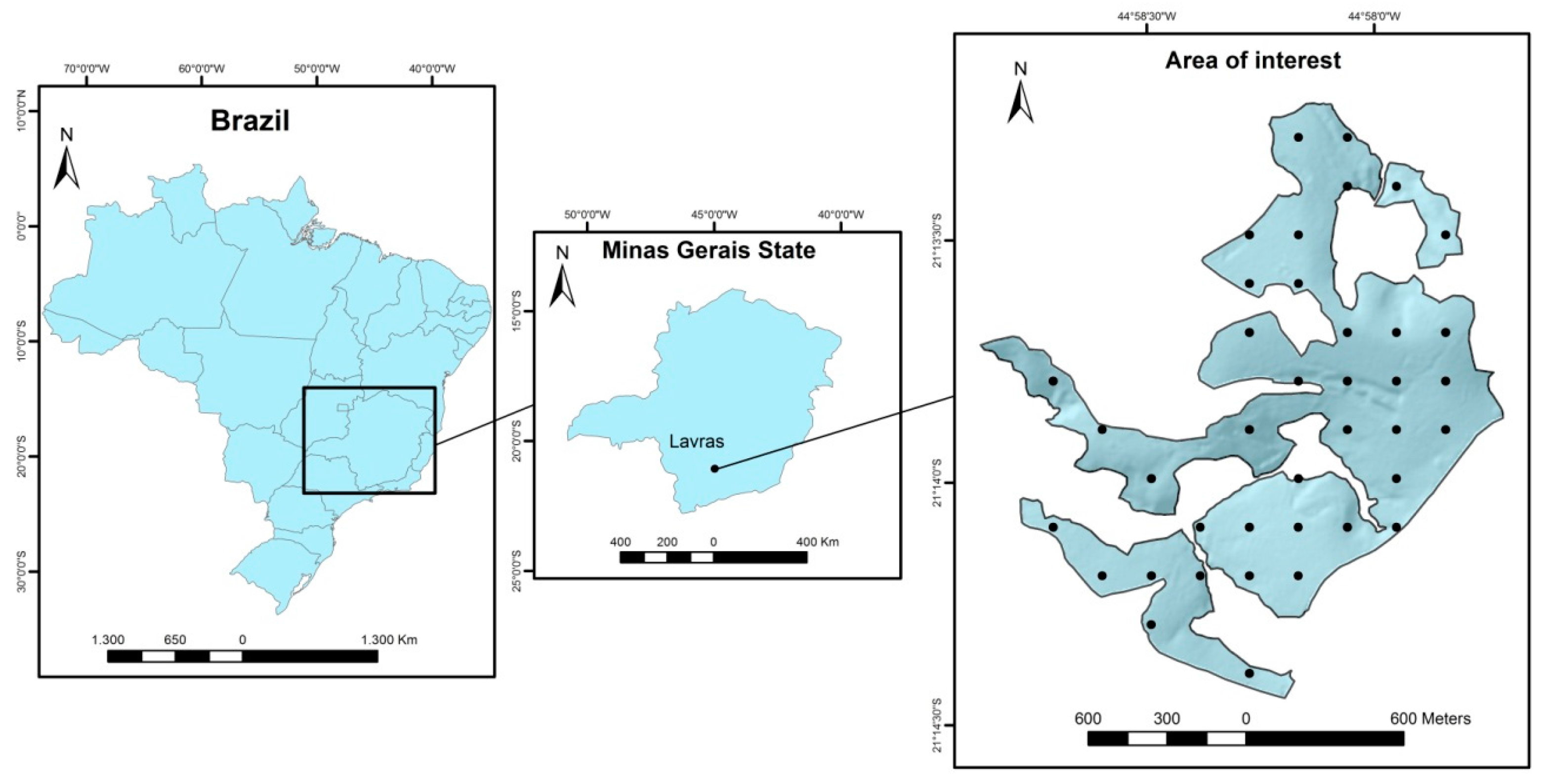
The study was carried out in an area located on the Campus of Federal University of Lavras, which is dominated by Latosols (Oxisols), a class representing the majority of the soils of Southern Minas Gerais state, Brazil (Figure 1). This area (~150.18 ha) does not have either a detailed soil map or a detailed geologic map and is located between latitudes 7,651,207 and 7,653,478 m and longitudes 501,962 and 503,957 m, Zone 23 K. The climate of the region is Cwa (C: subtropical climate; w: rainy summers; a: warm summers), characterized by rainy and warm summers and cold and dry winters, according to the Köppen classification system, with mean annual temperature and rainfall of 19 °C and 1530 mm, respectively [40].

The area encompasses a great geologic variety, with the dominance of leucocratic and mesocratic gneisses, the latter containing greater contents of Fe and darker minerals than the former, as well as a gabbro intrusion and sediments of varying nature.

A total of 39 sampling sites were selected throughout the study area, in a regular-grid design with a distance of 200 m between samples (Figure 1), covering different land uses, which included cultivated (pasture (signal grass) and coffee), and non-cultivated areas (native vegetation, semiperennial tropical forest). At each location, soils were classified according to the Brazilian Soil Classification System [41] into typic Dystrophic Yellow Latosol (LA), typic Dystrophic Red-Yellow Latosol (LVA), both developed from leucocratic gneiss, typic Dystrophic Red Latosol developed from mesocratic gneiss (LVm) and typic Dystropherric Red Latosol developed from gabbro (LVg). Such soils were classified as Latosols due to the presence of the B latosolic diagnostic horizon (similar to the oxic horizon in the U.S. Soil Taxonomy), followed by the dominant color of the B horizon (Munsell color 2.5YR or redder (red), 7.5YR or yellower (yellow), in between 2.5YR and 7.5YR (red-yellow)). The term Dystrophic is used when base saturation is smaller than 50%, whereas Dystropherric describes a dystrophic soil with Fe₂O₃ contents (obtained through a sulfuric acid digestion) ranging from 18% to 36%. The expression “typic” is used for reporting no intergrade regarding other soil classes.

Soil samples were collected from A and B horizons and submitted to analyses of particle size distribution by the pipette method [42,43]. Briefly, the sand fraction was separated using a 0.05-mm sieve; the silt and clay fractions were separated from each other after the sedimentation of the silt fraction, by pipetting a volume of the solution containing only the clay fraction, followed by oven-drying the solution and weighting the remaining clay fraction; the silt fraction is obtained by subtracting the weights of sand and clay fractions from the total weight of the soil. Chemical analyses included: soil pH (water, at 1:2.5 ratio); exchangeable Ca²⁺, Mg²⁺ and Al³⁺ extracted with 1 mol·L⁻¹ KCl [44]; available K and P extracted with Mehlich-l solution [45], H⁺ + Al³⁺ using the SMP extractor [46]; organic carbon by wet oxidation with potassium dichromate in sulfuric acid medium; and remaining P [47].

Table 1. Mean values of the physical and chemical properties of the soils sampled.

Soil Properties	LA 1 (2)		LVA 1 (10)		LVm 1 (16)		LVg 1 (11)
	Horizons
	A	B	A	B	A	B	A	B
pH	5.6	5.7	5.5	5.1	5.9	5.4	6.0	5.1
K (mg·dm−3)	122.0	15.0	153.0	19.6	176.9	30.6	166.4	30.2
P (mg·dm−3)	7.6	0.4	5.2	0.6	8.7	1.2	20.8	1.0
Ca2+ (mg·dm−3)	3.2	1.6	3.0	1.1	5.1	2.2	4.3	0.9
Mg2+ (mg·dm−3)	1.5	0.3	1.0	0.3	2.0	0.4	1.8	0.2
Al3+ (cmolc·dm−3)	0.0	0.1	0.3	0.4	0.1	0.2	0.2	0.3
H+ + Al3+ (cmolc·dm−3)	2.1	1.7	4.5	3.5	3.3	3.8	3.7	4.5
SB 2 (cmolc·dm−3)	5.0	1.8	4.4	1.4	7.6	2.7	6.5	1.2
t 3 (cmolc·dm−3)	5.0	1.9	4.6	1.7	7.6	2.8	6.7	1.5
T 4 (cmolc·dm−3)	7.1	3.5	8.9	4.9	10.9	6.5	10.2	5.7
V 5 (%)	70.3	52.0	56.4	34.7	67.3	43.3	64.1	23.4
m 6 (%)	0.0	3.1	6.2	24.4	1.4	11.4	4.8	19.1
SOM 7 (%)	3.7	1.1	5.6	1.5	6.5	2.1	6.6	2.8
P-Rem (mg·dm−3)	26.6	9.8	23.1	7.3	20.2	7.2	15.6	3.1
Clay (g·kg−1)	470.0	540.0	451.0	566.0	501.0	595.0	535.0	659.0
Silt (g·kg−1)	140.0	85.0	18.2	119.0	230.0	158.0	312.0	186.0
Sand (g·kg−1)	390.0	375.0	367.0	315.0	269.0	247.0	153.0	155.0

¹ LA: Yellow Latosol; LVA: Red-Yellow Latosol; LVm: Red Latosol developed from mesocratic gneiss; LVg: Red Latosol developed from gabbro. Numbers between parentheses show the number of soil samples classified as those soil classes; ² SB: sum of bases; ³ t: effective cation exchange capacity; ⁴ potential cation exchange capacity; ⁵ V: base saturation; ⁶ m: aluminum saturation; ⁷ SOM: soil organic matter.

presents the physical and chemical characterization of soils developed from each parent material.

Magnetic susceptibility per unit of mass (χ_BF) was determined using the Barrington MS2B magnetometer in air-dried samples passed through a 2-mm sieve. Data were obtained at low frequency (χ_BF = 0.47 kHz) and calculated through the expression χ_BF = (10 × κ) m⁻¹, where κ is dimensionless [48]; studying different soils and parent materials in the region of Lavras, it was noticed that soil classes comprising the same taxonomic order (Latosols and Argisols) developed from different parent materials showed contrasting magnetic susceptibility values, which demonstrates the potential of using magnetic susceptibility for characterizing soils with varying parent materials.

For the analyses of total elemental contents in soil samples, a portable X-ray fluorescence analyzer (pXRF) (Bruker model S1 Titan LE) was used to scan samples that were previously air-dried and passed through a 2-mm sieve. Samples were placed in plastic holders, and the scanning was performed during 60 s in two beams. The software used in pXRF is GeoChem General, and the device contains a 50-kV and 100-µA X-ray tube, which provides fairly selective detection of various elements, ranging from Mg to U, with limits of detection (LOD) in the parts per million range (ppm) for many of these elements. Calibration of the pXRF was checked with the analysis of a standard soil sample (CS). The average of the measured values for selected elements found in CS was within acceptable limits: Al₂O₃ (99%), SiO₂ (95%), K₂O (90%), Mn (85%), Fe (130%) and Cu (93%). Furthermore, quality control and quality assurance protocols were performed by analyses of NIST Standard Reference Materials with varying elemental concentrations (SRM 2710a and SRM 2711a). Each of these control samples (NIST and CS) were analyzed ten times. The recoveries (%) for NIST 2710a and NIST 2711a were, respectively: Al (36; 69), Si (46; 41), P (75; 22), K (67; 33), Ca (76; <LOD), Ti (77; 55), V (155; 135), Mn (87; 55), Fe (92; 77), Cu (110; 104), Zn (129; 135) and Zr (257; 54). Selected data obtained with pXRF for the 39 samples collected in the field (MgO, SiO₂, Cl, K₂O, Ti, Fe, Zn, Zr, Mn, Cr, Ni, Cu and Ce) were used as covariates to help soil and geologic mapping.

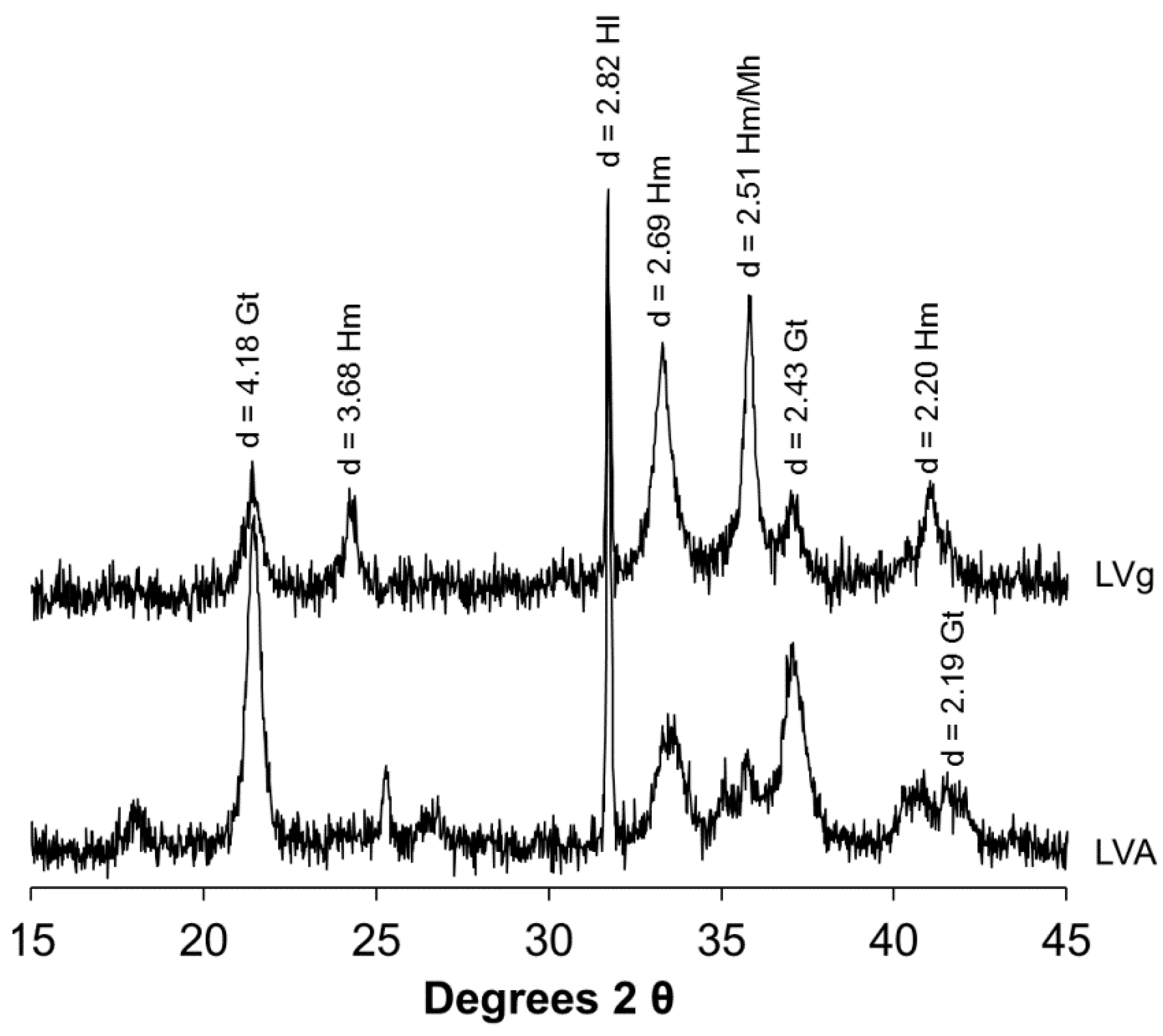
X-ray diffractometry (XRD) analyses were performed to identify Fe oxide minerals present in the soil clay fraction, which was previously treated with 5 mol·L⁻¹ NaOH [49] for iron concentration and dissolution of kaolinite, gibbsite and other minerals in the samples. Afterwards, non-oriented plates (Koch plate) were prepared for XRD analyses in the range from 15 to 45°2θ, using halite as an internal pattern to correct for instrumental distortions.

2.2. Soil Classes Mapping

A digital elevation model (DEM) of 5-m resolution was created from contour lines of 1 m of vertical distance by the Topo to Raster function in ArcGIS 10.1(ESRI). From this DEM, 9 terrain variables commonly used for predictions and mapping of soil classes and properties [10,50,51,52,53,54,55] were selected using both ArcGIS 10.1 and SAGA GIS [56], including: slope, topographic wetness index (TWI), SAGA wetness index (SWI), cross-sectional and longitudinal curvatures, vertical distance to channel network and valley depth, in addition to elevation and Geomorphons [57]. Geomorphons consist of an algorithm that classifies the landscape into 10 possible landforms, and thus, it is expected to contribute to distinguishing geomorphology patterns that may be related to varying soil classes and properties.

Terrain information in addition to magnetic susceptibility and pXRF data for the 39 sites were grouped into four soil classes found in the study area during the field work, and box plots were generated in order to help identify the variables (terrain and laboratory data) that contributed the most to distinguishing soil classes. Similar boxplot analyses have been performed by [52,58,59,60] to identify the best variables regarding the prediction of soil properties. In this procedure (analysis of boxplots), the variables whose values per soil class presented different ranges, without overlapping the range of values of other soil classes, were considered appropriate to distinguish soil classes and, hence, adequate to be used for soil mapping.

Next, the mean value of these previously-mentioned variables was calculated per each soil class, being considered representative of the typical condition for each soil class of occurrence. The standard deviation of each variable for each soil class was also calculated per soil class based on data obtained from the 39 sampling sites. Both the mean and the standard deviation of the chosen variables per soil class were used as rules for predicting the spatial occurrence of soil classes through ArcSIE, the soil inference function, an ArcGIS extension that has been successfully used for soil mapping [59,61,62,63,64]. For example, according to the sampling sites, a soil class was found to occur at places where slope values range from 12% to 20% (mean ± standard deviation), with a mean value (typical condition) of 16% coupled with SWI ranging from 2 to 4 and a mean value of 3. Based on this kind of information (rules, typical conditions and range of values of variables for all of the soil classes occurring in the area), ArcSIE uses fuzzy logic and similarity vectors to predict soil classes and properties on the landscape [65] identifying the places that are more related to the typical conditions of each soil class. For that, ArcSIE generates membership maps in raster format in which every pixel shows the value of similarity to a typical condition, ranging from 0 (low similarity) to 1 (great similarity). Subsequently, a final map is generated representing the places that are more likely for each soil class to occur, according to the rules inserted into ArcSIE.

For the soil mapping procedure, DTM information was continuously available for the entire study area, but variables obtained from pXRF and magnetic susceptibility data at the 39 sampled sites needed to be extrapolated to the entire area using the inverse distance weighting (IDW) method, with the purpose of being used as continuous variables for soil mapping through ArcSIE. The values inferred at non-sampled areas by IDW are estimated using a linear combination of values at the sampled points, weighted by an inverse function of the distance from the point of interest to the sample points. The weights (λ_i) are expressed as:

$${\mathsf{\lambda }}_i= \frac{\frac{1}{d_i^p}}{{\sum }_{i=1}^n\frac{1}{d_i^p}}$$

(1)

where $d_i$ is the distance between $x_0$ and $x_0$, p is a power parameter and n represents the number of sampled points used for the estimation. This interpolation was performed in ArcGIS 10.1 (ESRI), where a power parameter equal to 2 (default) was chosen. Mean error (ME) and root mean square error (RMSE) were calculated for assessing the accuracy of interpolation, as follows:

$$ME= \frac{1}{n}{\displaystyle \sum }_{i=1}^n\left(ei-mi\right)$$

(2)

$$RMSE=\sqrt{\frac{1}{n}{\displaystyle \sum }_{i=1}^n{\left(ei-mi\right)}^2}$$

(3)

where n is the number of observations, ei is the estimated value from pXRF and magnetic susceptibility data and mi is the correspondent measured value.

The accuracy assessment of the soil classes map generated in ArcSIE was performed through the comparison of the soil class presented on the map with the real soil class at 14 places (field validation) randomly chosen within the study area. From this analysis, overall accuracy (percentage of correctly-predicted soil classes), Kappa index, omission and commission errors and user’s and producer’s accuracy were calculated for each soil class. The formulas for calculating the Kappa index and producer’s and user’s accuracies are presented below:

$$Kappa= \frac{Po-Pe}{1-Pe}$$

(4)

where Po is the proportion of correctly-classified samples and Pe is the probability of random agreement. The Kappa index ranges from −1 to 1, although the results are commonly found between 0 and 1,indicating increasing accuracy as the values get closer to 1 [66]:

$$User’s accuracy= \frac{Xii}{{\sum }_{i=1}^{r}Xij}$$

(5)

$$Producer’s accuracy= \frac{Xjj}{{\sum }_{j=1}^{r}Xij}$$

(6)

where X_ii and X_jj represents the number of correctly-classified samples and X_ij indicates the total number of samples of a soil class in a row (user’s accuracy) or column (producer’s accuracy) of a confusion matrix.

2.3. Soil Particle Size Distribution Predictive Models

The ordinary least square multiple linear regression (OLS) was used for fitting the prediction models of sand and clay contents (dependent variables) in ArcGIS 10.1 from proximal sensors, DTM and the previously obtained soil classes map (explanatory variables). First, the exploratory analysis module was applied to the data to provide a suitable set of explanatory variables, to determine if the OLS assumptions were met and to measure the prediction power of the candidate variables in order to generate effective and reliable prediction models. Only models that met the criteria were considered as suitable models. Statistically-significant explanatory variables, models with higher adjusted R², Akaike’s information criterion, multicollinearity checked by means of the variance inflation factor, the normality of regression residuals and parsimony were all carefully considered and analyzed for the selected models.

In order to properly assess the accuracy of the models, independent sand and clay datasets were used. Such data were not used for developing the models. Mean error and root mean square of prediction error were calculated, according to Equations (2) and (3), as previously mentioned. Furthermore, in order to assess the predictive power of the variables, five types of prediction models were refined for clay and sand contents, according to the explanatory variable source: (i) only with DTM; (ii) proximal sensors plus parent material (based on soil classes map); (iii) proximal sensors plus parent material plus DTM; (iv) only proximal sensors; and (v) proximal sensors plus DTM.

3. Results

3.1. Digital Soil Mapping

Boxplots of the analyzed variables are shown on Figure 2. The fluorescence energy is characteristic of the elements present in a sample of interest, and so, theoretically, the spectrum of atomic weights greater than 19 May be determined by the pXRF detector. However, because of low energy responses, not all elements of the periodic table can be effectively measured, and there is also a limit of detection depending on the content of the element of interest in the sample [67]. pXRF could identify 13 elements and/or compounds for at least one soil class, increasing the number of potentially useful variables to distinguish different Latosols, making up a total of 23 variables, including both the ones related to terrain features and those obtained from laboratory analyses (pXRF and magnetic susceptibility). Only elements with low error or uncertainty were selected. This error is a deviation calculated by the equipment, according to its calibration. Four out of the 23 variables were considered more capable of distinguishing at least one of the four possible soil classes (Figure 2), according to the boxplots, three of them being related to proximal sensing analyses (magnetic susceptibility, Fe and SiO₂) and one related to terrain (SWI). Regarding all of the terrain-related variables, only SWI presented high potential for distinguishing a soil class (LA) due to the lowest values found for that soil class in comparison with the others. In contrast, all of the other terrain-related variables contain values within a similar interval among the four soil classes.

Magnetic susceptibility, Fe and SiO₂ contents presented distinguished ranges of values for the soil classes, in addition to SWI. Soils derived from gabbro had higher magnetic susceptibility and Fe contents, while LA presented the greatest concentration of SiO₂. Other chemical compounds were not considered adequate for distinguishing one soil class from the others because they could be estimated only in some soil classes (e.g., Ni, Cr, Cu, Ce and MgO) or because their values were within the same range for all soil classes (K₂O, Ti, Mn, Cl, Zn and Zr).

Redder soils (LVA, LVm and LVg) had greater contents of Fe and Ti and some elements that were not present in LA, such as Ni, Cr and Cu. This latter soil class contains MgO and Ce, which were not detected by pXRF for the other soils, and greater amounts of SiO₂ and Cl than the redder soils.

Table 2. Mean and standard deviation (SD) of the variable values.

Variable	LA	LVA	LVm	LVg
MS 1 (10−7 m3·kg-1)	4.8	15.7	43	194
SM SD	0.26	16.9	27	97
MgO (ppm)	23,545	-	-	-
MgO SD	20,543	-	-	-
SiO2 (ppm)	19,568	17,265	16,946	16,289
SiO2 SD	1870	1858	1961	2033.7
Cl (ppm)	1461	1160	1113	984.9
Cl SD	36	40	48.6	60.8
K2O (ppm)	1432	1397	1324	945
K2O SD	146	150	159.2	157.9
Ti (ppm)	5900	6799	8379	9221
Ti SD	155	165	186.2	196.7
Fe (ppm)	31,880	46,103	66,450	96,410
Fe SD	304	358	439.6	531
Zn (ppm)	18	23	35.3	32.2
Zn SD	8	9	9.8	10.7
Zr (ppm)	170	187	182	167.6
Zr SD	9	10	10.8	11.6
Mn (ppm)	91	152	372	-
Mn SD	53	62	79.3	-
Cr (ppm)	-	-	454	1103
Cr SD	-	-	55.9	68.3
Ni (ppm)	-	-	121	105.7
Ni SD	-	-	23.5	28.1
Cu (ppm)	-	-	29	36.8
Cu SD	-	-	9.6	11.3
Ce (ppm)	1538	-	-	-
Ce SD	468	-	-	-

¹ Magnetic susceptibility.

shows the mean and the standard deviation of the variable values obtained by analyses of the soil samples grouped according to the soil class. It can be noticed that the greatest magnetic susceptibility, as well as Fe and Ti contents were found for LVg, followed by LVm, and also that they decreased as the soil became yellower. On the other hand, SiO₂, Cl and K₂O contents decreased as the soil became redder. Zn and Zr contents were greater for LVm and LVA, respectively.

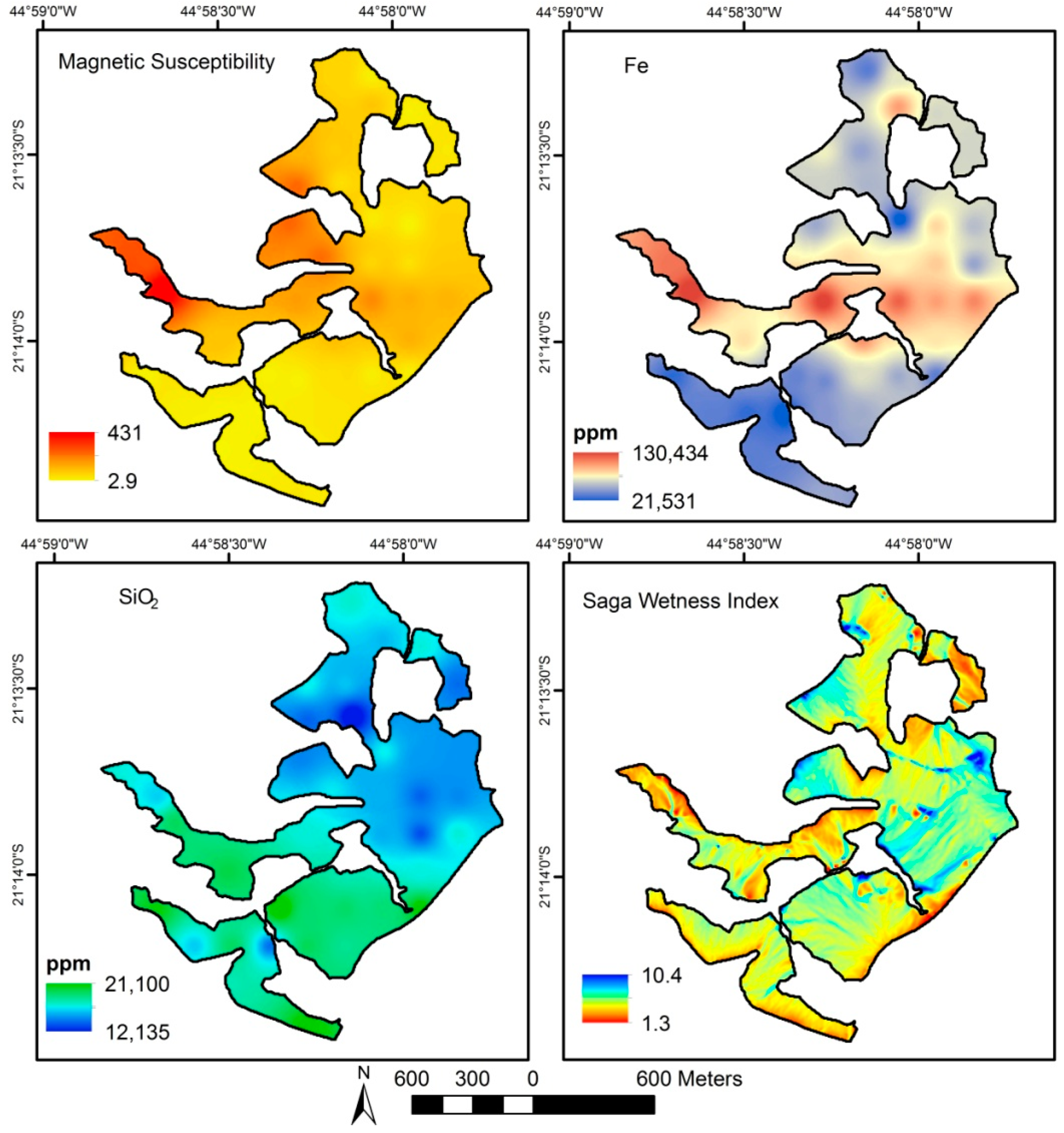
Figure 3 shows the maps of the four variables considered more capable of distinguishing the soil classes. Magnetic susceptibility ranged from 2.9 to 431 χ_BF in the study area, and higher values covaried with larger contents of Fe, which, in turn, ranged from 21,531 to 130,434 ppm. SiO₂ contents ranged from 12,135 to 21,100 ppm, while SWI ranged from 1.3 to 10.4, being greater as the chance of accumulating water increases on the landscape [68]. The accuracy indexes of magnetic susceptibility, Fe and SiO₂ IDW maps were, respectively: ME = −3.603 and RMSE = 60.604; ME = −340.103 and RMSE = 22,867.917; ME = −137.973 and RMSE = 1707.471.

Table 3. Values used in ArcSIE in order to map the soil classes’ distribution in the study area. SWI, SAGA wetness index.

	Similarity 1	LA	LVA	LVm	LVg 2
	50%	31,610	23,100	48,450	70,410
Fe	100%	31,880	46,100	66,450	96,410
	50%	32,150	69,100	84,450	-
	50%	18,840	14,970	14,750	-
SiO2	100%	19,570	17,270	16,950	-
	50%	20,300	19,570	19,150	-
	50%	4.54	-	16	97
SM	100%	4.80	-	43	194
	50%	5.06	-	70	-
	50%	2.9	-	-	-
SWI	100%	3.0	-	-	-
	50%	3.1	-	-	-

¹ Similarity to the typical condition. ² The curve type for LVg is S-shaped, while for other soils, it is bell-shaped.

represents the values used in ArcSIE to generate the soil class map. The similarity column in Table 3 represents the similarity to the typical condition: when it is 100%, it corresponds to the typical condition for a soil class to occur (mean value obtained from the collected samples), whereas 50% represents the values resulting from the standard deviation subtracted from (lower limit) and added to (upper limit) the mean value, indicating the range of values for a soil class to occur, with at least 50% membership in relation to the typical condition. Data in Table 3 show that Fe was the unique variable used for mapping all four soil classes, while the other three variables were employed for at least one soil class, such as SWI, although in all cases, a soil class required more than one variable to be mapped.

The geologic variety contributed to the formation of Latosols with contrasting physical, chemical and mineralogical properties [7,48,69], as shown in Table 1 and Figure 4. Leucocratic gneisses tend to form Yellow- or Red-Yellow Latosols, while mesocratic gneisses develop Red Latosols, as well as the gabbro-derived soils, yet the latter contain different properties in relation to the former, such as the presence of maghemite (Figure 4), higher Fe contents and magnetic susceptibility values (Table 2).

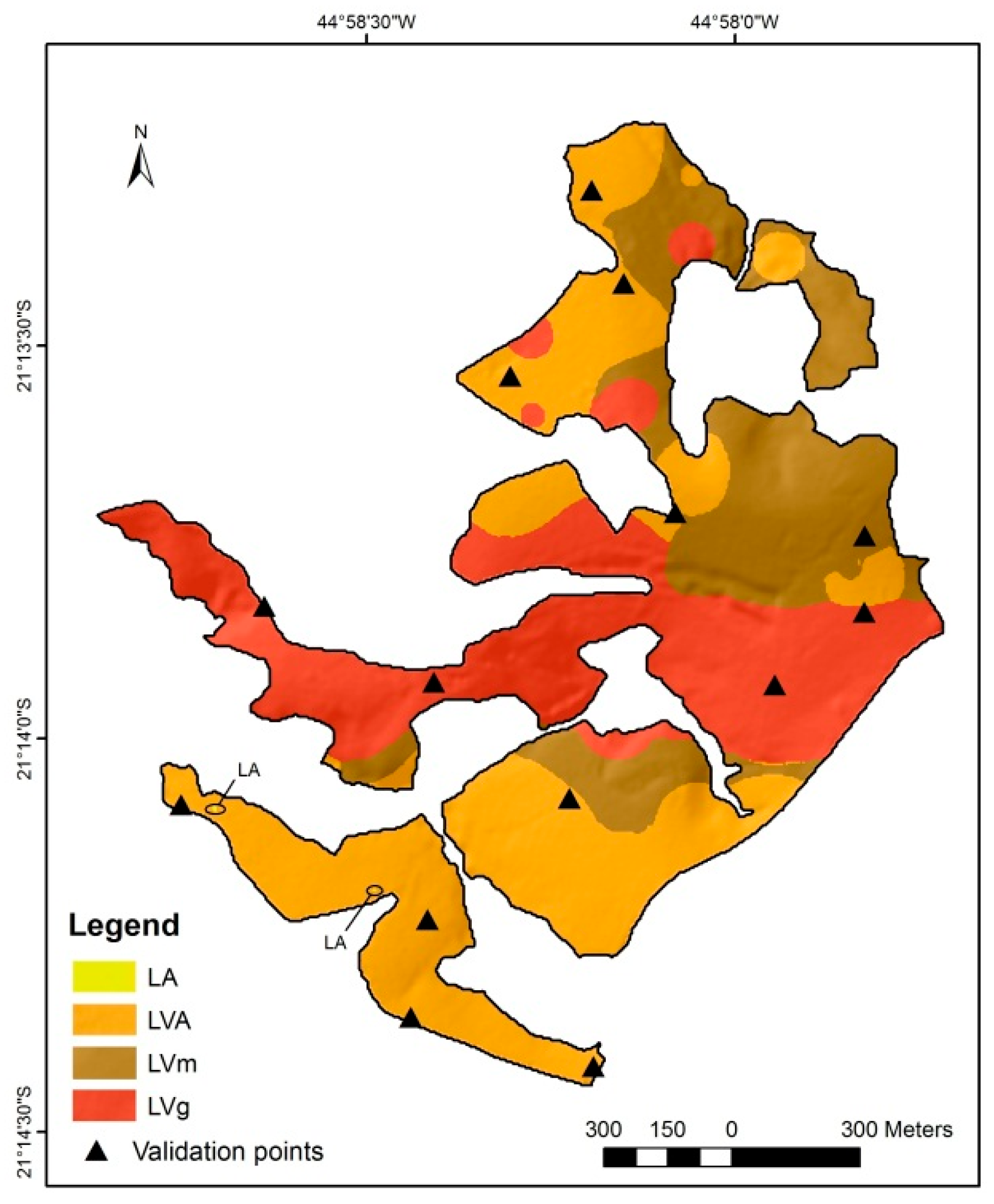
The predicted soil map is shown in Figure 5. It can be noticed that LVA is the soil class that occupies the largest portion of the area, corresponding to 40.79% (61.25 ha). It is followed by LVg, with 33.70% (50.60 ha), mainly occurring in the center of the study area, from east to west. In sequence, LVm is found in 25.50% (38.30 ha). Lastly, LA occurs in 0.01% (0.016 ha) of the area, at places where SWI is lower.

The indexes for the predicted soil map accuracy were assessed according to a confusion matrix (

Table 4. Confusion matrix, omission and commission errors and producer’s and user’s accuracies for the predicted soil map.

	LVg	LVm	LVA	LA	Omission Error	Producer’s Accuracy	Commission Error	User’s Accuracy
LVg	4	0	1	0	0	100	20	80
LVm	0	2	2	0	0	100	50	50
LVA	0	0	5	0	37.5	32.5	0	100
LA	0	0	0	0	0	100	0	100

), from where it was found an overall accuracy of 78.57%, meaning that 11 out of the 14 validation points match the predicted soil class. The validation resulted in a Kappa index of 0.6719, corresponding to a substantial classification [66]. Furthermore, the omission error for LVA was the greatest (lowest producer’s accuracy), while commission error was the greatest for LVm (lowest user’s accuracy).

3.2. Soil Particle Size Distribution Predictive Models

Table 5. Ordinary least square multiple linear regression models of the parameters for clay content developed from proximal sensors (PS) portable X-ray fluorescence and magnetic susceptibility, parent material (PM) and digital terrain models (DTM).

Explanatory Variable	Clay (PS + PM) and Clay (DTM + PS + PM)			Clay (PS)			Clay (DTM + PS)
	Coefficient	VIF 1	Variable Significance (%)	Coefficient	VIF	Variable Significance (%)	Coefficient	VIF	Variable Significance (%)
Intercept	72.177			92,361			79,406
MS 2	-		67.75	0.028 *	1.980	76.77	0.035 **	1.347	79.95
SiO2	-		6.85	-	-	10.10	-	-	8.09
Cl	-		100.00	−0.012 **	1.311	100.00	-	-	100.00
K2O	−0.013 **	1.334	100.00	−0.010 **	1.313	100.00	−0.009 **	1.363	100.00
Ti	−0.001 *	1.750	4.84	-	-	0.00	-	-	6.12
Fe	-		9.58	−0.00005 **	1.803	3.03	-	-	11.90
Zn	−0.196 **	1.213	77.43	−0.164 **	1.146	87.88	−0.165 **	1.101	70.29
Zr	0.038 *	1.310	11.54	-	-	8.08	-	-	11.35
Geomorphons	-		4.84	-	-	-	-	-	0.27
DEM 3	-		9.58	-	-	-	-	-	8.97
SWI 4	-		13.81	-	-	-	-	-	12.85
WI 5	-		5.62	-	-	-	-	-	4.89
Slope	-		70.17	-	-	-	−0.372 *	1.173	64.65
AACHN 6	-		4.84	-	-	-	-	-	2.31
Valley depth	-		9.58	-	-	-	-	-	5.30
Parent material	4.527 **	1.740	67.75	-	-	-	-	-	-
R2	0.66			0.71			0.67
Adjusted R2	0.61			0.67			0.64

¹ VIF, variance inflation factor; ² MS, magnetic susceptibility; ³ digital elevation model; ⁴ SWI, SAGA wetness index; ⁵ WI, wetness index; ⁶ AACHN, altitude above the channel network; model variable significance: * = 0.05, ** = 0.01.

and

Table 6. Ordinary least square multiple linear regression models of parameters for sand content developed from proximal sensors (PS) portable X-ray fluorescence and magnetic susceptibility, parent material (PM) and digital terrain models (DTM).

Explanatory Variable	Sand (PS + PM)			Sand (DTM + PS + PM)			Sand (PS)			Sand (DTM + PS)
	Coefficient	VIF 1	Variable Significance (%)	Coefficient	VIF	Variable Significance (%)	Coefficient	VIF	Variable Significance (%)	Coefficient	VIF	Variable Significance (%)
Intercept	−1.726			0.487648			−30,497			9.134
MS 2	-		47.85	-		72.13	-	-	78.79	−0.036 **	1.708	92.11
SiO2	0.001 *	1.278	78.53	0.001 *	1.337	61.88	0.001 **	1.218	85.86	0.001 **	1.103	63.83
Cl	0.013 **	1.322	100.00	0.012 **	1.334	99.95	0.017 **	1.202	100.00	-	-	99.93
K2O	-		27.61	-		39.98	-	-	34.34	-	-	49.22
Ti	-		6.13	-		13.70	−0.001 *	1.157	10.10	-	-	17.61
Fe	-		59.51	-		78.52	-	-	90.91	−0.0001 **	1.825	94.09
Zn	-		1.23	-		5.00	-	-	2.02	-	-	6.59
Zr	0.050 *	1.121	16.56	0.046 *	1.130	24.32	0.101 **	1.173	22.22	-	-	28.96
Geomorphons	-		-	-		3.45	-	-	-	-	-	4.42
DEM 3	-		-	-		47.45	-	-	-	-	-	50.44
SWI 4	-		-	-		11.03	-	-	-	-	-	10.67
WI 5	-		-	-		7.52	-	-	-	-	-	9.11
Slope	-		-	0.270 *	1.076	47.45	-	-	-	0.432 **	1.122	32.29
AACHN 6	-		-	-		5.20	-	-	-	-	-	6.12
Valley depth	-		-	-		5.36	-	-	-	-	-	6.80
Parent material	−5.154 **	1.333	100.00	−5.560 **	1.380	99.64	-	-	-	-	-	-
R2	0.73			0.77			0.63			0.69
Adjusted R2	0.70			0.73			0.58			0.66

¹ VIF, variance inflation factor; ² MS, magnetic susceptibility; ³ digital elevation model; ⁴ SWI, SAGA wetness index; ⁵ WI, wetness index; ⁶ AACHN, altitude above the channel network; model variable significance: * = 0.05, ** = 0.01.

show, respectively, the parameters of clay and sand predictive models from OLS multiple linear regression, as well as the R², adjusted R², the variance inflation factor (VIF) and the summary of variable significance. VIF less than 7.5 means no redundancy among explanatory variables. The summary of variable significance provides information about variable relationships and how consistent those relationships are. For each explanatory variable, the OLS tool calculates a coefficient to determine if such a variable can help to explain clay and sand contents. These coefficients (and their statistical significance) can be changed depending on the combination of variables in the model. The summary of variables’ significance provides information about variable relationships and how consistent those relationships are. Larger values (%) mean stronger predictors, as they were considered statistically significant in most of the cases during the analysis, i.e., they are consistently significant, and the relationships are stable. All equations are models that met the OLS requirements. Considering the adjusted R², the models are considered suitable, since all of them were able to explain more than 58% of the total variance, with sand models performing better than clay models. However, adjusted R² is not the unique parameter that determines the modeling performance. All of the explanatory variables were statistically significant, and all of the residuals of regression showed normality.

Differently from the digital soil map, only SiO₂, Cl, K₂O, Ti, Fe, Zn and Zr from pXRF were used for developing models, because their contents were above the detection limit for all sampling points. The models that had only DTM as explanatory variables did not meet the OLS requirements, with adjusted R² around 0.15.

Proximal sensors showed higher predictive power and consistency (higher variable significance) than DTM, with no multicollinearity among them. TWI, SWI and valley depth showed multicollinearity, while proximal sensors and parent material did not present multicollinearity. Parent material was statistically significant (0.01 level) in most cases (variable significance), which reinforces the importance of soil class and parent material for the prediction of soil properties, such as soil particle size distribution. For the prediction of clay content, Fe and magnetic susceptibility were selected in the models that did not consider parent material (models using only proximal sensors and proximal sensors plus DTM). Considering the adjusted R², the model with proximal sensors showed greater predictive power. However, for the prediction of sand content, models that excluded parent material showed lower adjusted R².

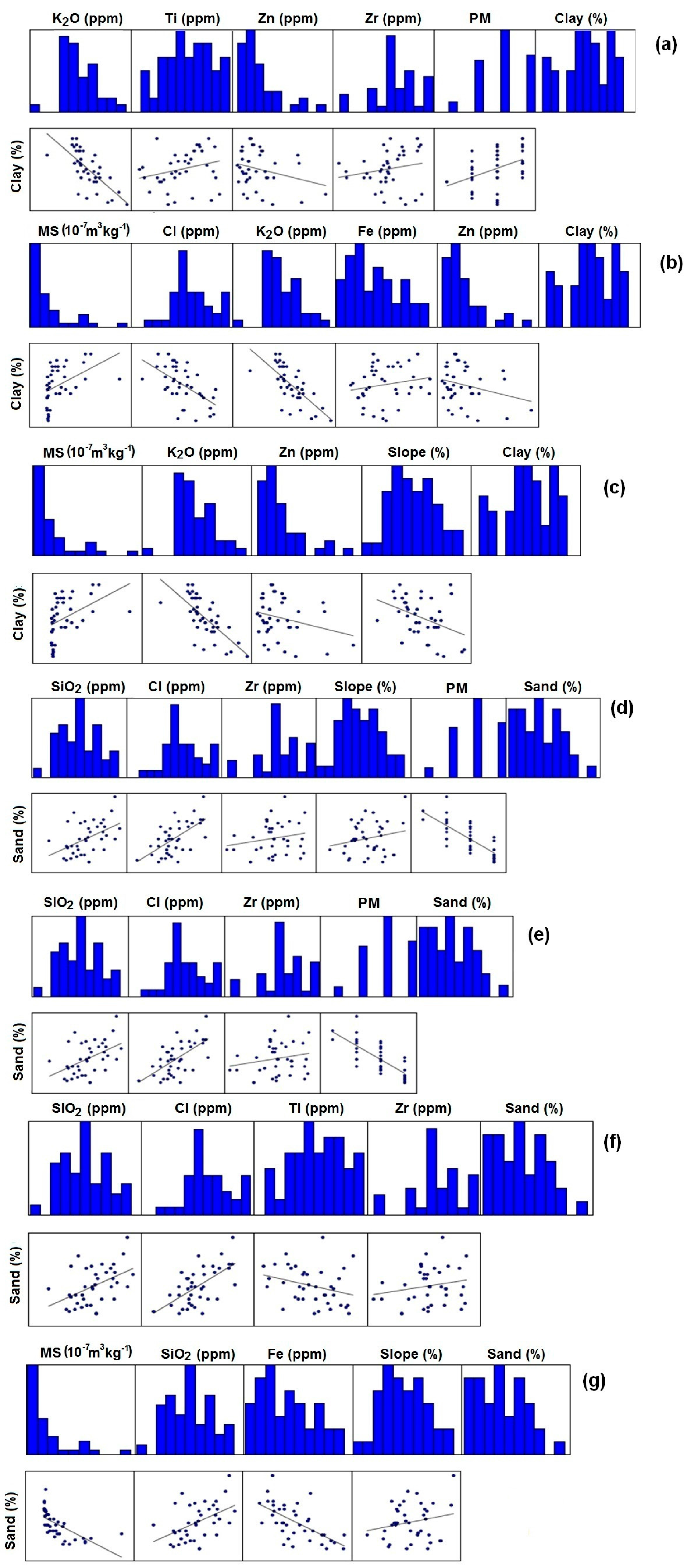
Considering the selected explanatory variables and the scatterplot graphics (Figure 6), clay content values increase as follows: leucocratic gneiss → mesocratic gneiss → gabbro. This was followed by increasing Ti and decreasing K₂O and Zn contents. Sand content increases according to the sequence gabbro → mesocratic gneiss → leucocratic granite gneiss, followed by increasing SiO₂, Zr and Cl contents.

Table 7. Accuracy assessment of predictive clay and sand models.

Model	ME	RMSE	R2
Clay (PS 1 + PM 2) and (DTM 3 + PS + PM)	13.56	3.68	0.52
Clay (PS)	2.21	6.26	0.39
Clay (DTM + PS)	−4.32	12.37	0.37
Sand (PS + PM)	25.84	5.08	0.69
Sand (DTM + PS + PM)	24.11	4.91	0.67
Sand (PS)	48	136.47	0.72
Sand (DTM + PS)	−10.81	30.41	0.87

¹ PS, proximal sensor; ² PM, parent material; ³ DTM, digital terrain model.

shows the accuracy of the models, from an independent dataset. In general, the R² are higher than 0.50, and the models presented a positive bias (positive ME), with small RMSE, which means high accuracy. The R² of clay content is the lowest considering scatterplots; on the other hand, the ME and the RMSE are the lowest. In general, when compared to the validation indexes from other studies that used proximal sensors, the models in our study performed well. In the studies of [33,70,71,72], the RMSE values range from 2.66 to 7.9, which is similar to the RMSE values of our study.

4. Discussion

4.1. Soil Classes Mapping

Through the analysis of boxplots (Figure 2), it can be noticed that the terrain attributes most commonly used for the predictions of both soil classes and properties were not capable of solely distinguishing most Latosols in the study area, except for SWI, which could distinguish LA from the other Latosols.

The magnetic susceptibility data and some elements/compounds assessed by the pXRF technique, mainly SiO₂ and Fe, could aid in predicting soil classes, probably because of their relationships to soil parent material [73]. The work in [48], studying eight soils and their correspondence to the parent material in the region of Lavras, found that a gabbro-derived soil contained higher contents of Fe₂O₃ and magnetic susceptibility value and a lower content of SiO₂ when compared to soils derived from gneiss, which agrees with the findings of our study, as estimated here by pXRF.

Among the gneisses, soils derived from mesocratic ones are expected to contain higher contents of Fe and lower contents of SiO₂, in comparison with soils derived from leucocratic gneisses, as supported by our pXRF analyses (Table 2). Similar results were found by [7,8], studying soils of the same region.

Regarding magnetic susceptibility, [74] found lower values of magnetic susceptibility in soils derived from rocks, such as gneiss, granite, quartzite, marble and dolomite, due to their lower content of Fe when compared to soils derived from mafic rocks. The presence of gneiss, granite, quartzite, marble and dolomite reduces the chances of ferromagnetic minerals to be formed [75], which is in agreement with the lower Fe content and magnetic susceptibility values found for gneiss-derived soils (LA, LVA and LVm) in comparison to the gabbro-derived soil (LVg) found in our study. Those authors also found higher magnetic susceptibility values for soils derived from diabase and basalt, the latter being the extrusive rock correspondent to gabbro, ranging from 225 to 7790 × 10⁻⁸ m³·kg⁻¹, which contributed to the distinction of those soils from other soils derived from different parent materials. The work in [76], studying magnetic susceptibility in samples of soils derived from sandstone and basalt with the goal of separating soils from different landscape segments in the Jaboticabal region (São Paulo state, Brazil), found that this variable could help with the separation of soils derived from these two rock types.

The higher magnetic susceptibility value for LVg than for Latosols derived from gneiss is probably due to the presence of maghemite, as supported by the X-ray diffractograms (Figure 4). Contrary to magnetite and maghemite, generally found in the sand and clay fractions, respectively [77], goethite and hematite, also present in the studied soils, tend to contain null or low values of magnetic susceptibility [78], similarly to the findings of this study (Figure 4 and Table 3).

According to the soil map of the study area, LVA was the dominant class. This result was also reported by other works related to soil mapping in this same region, such as [79,80].

In Brazil, due to the lack of detailed soil surveys, the establishment of differential soil properties at inferior taxonomic levels has been discussed, and a consensus has not been reached yet. This might be one of the causes of the mismatches between taxonomical and mapping units in detailed soil maps in Brazil. In this sense, the importance of numerical classification models has increased as an alternative for mapping [26,81,82]. Keeping in mind such limitations and options to overcome it, this study proposes the use of numerical soil properties from proximal sensors, which could function as a basis for establishing the boundaries of different types of Latosols at lower taxonomic levels, coupled with a data mining tool for extracting and applying information.

According to the validation indexes, this approach properly fits to the study area, thus contributing to the identification of taxonomic units and their distribution through the landscape (mapping units). The accuracy assessment presented values of overall accuracy within the range defined by the Technical Manual of Pedology [83], which establishes the basis for soil surveys in Brazil, considering reliable soil maps those that present more than 70% of overall accuracy. The remaining 30% are considered inclusions of other soil classes within a mapping unit, which are not included in the legends of soil maps. Thus, the soil maps generated in this work can be considered adequate. Furthermore, soil maps have the ability to provide information about the spatial distribution of surficial geology [84], and, thus, such maps can be used for several soil property predictions, which was performed in this study for modeling soil particle size distribution, as an example.

4.2. Soil Particle Size Distribution Prediction Models

The main goal here was not only to develop soil particle size distribution prediction models, but also to understand which covariates (proximal sensors, DTM or soil classes map) could better explain this soil property, using the OLS multiple regression, a data mining tool [9]. From the OLS multiple linear regression results, it is clear that the soil class itself and the elemental composition obtained from pXRF that is related to parent material were the best explanatory variables, consistently increasing the prediction power of models.

Chemical elements obtained from pXRF were able to predict soil particle size distribution, which, in turn, depends on parent material, as well as on weathering and leaching [33]. Considering those explanatory variables of prediction models, as clay content increases, K₂O and Zn decreases, Ti increases and the soils tend to be Red Latosols derived from gabbro [73]. Although low K contents were found in those soils, which was expected due to the very low contents of K-bearing minerals in those parent materials and the intense and prolonged weathering-leaching processes to which those soils were subjected [73,85,86,87], there was a trend of reducing K content and increasing clay content (as an influence of parent materials) in soils developed from varying parent materials, following the sequence leucocratic gneiss → mesocratic gneiss → gabbro. The same trend of reducing K content and increasing clay contents was reported by [48], studying soils derived from the same parent materials of this current work. As sand content increases, SiO₂, Cl and Zr are greater, and the soils tend to be Yellow Latosols derived from leucocratic gneiss [8]. Cl was an important chemical component in the predictive models, and according to [88], Cl contents tend to be higher in igneous rocks. The same authors stated that Zr content in soils generally is inherited from parent rocks. SiO₂ content in the sand fraction was selected to be used on the models, probably because particles in the sand fraction in these extremely weathered-leached soils, such as those in tropical conditions, e.g., in Brazil, are by far dominantly composed of quartz, followed by other very resistant minerals in much smaller quantities, such as magnetite, concretions and nodules of Fe, as reported by [86].

Analyzing the low predictive power of DTM in the models, it is important to highlight that such maps serve only as a proxy of the current environmental conditions, which in many cases are different from the past conditions in which pedogenesis took place [6,89]. Considering that Latosols, soils formed in ancient landscapes, resulted from an environment of soil formation that does not currently exist [87], the contemporary landscape analyzed by DTM might not translate to the preterit soil-forming conditions [13]. Since DTM did not significantly improve the predictive power of soil properties’ prediction, it is preferable to create models that contain less independent variables, reducing time and cost for processing data. These findings suggest that, for tropical conditions, alternative variables that help the predictions of soil classes and properties, such as those provided by pXRF and magnetic susceptibility, may contribute to soils’ differentiation and, hence, for the creation/improvement of detailed soil maps, following the world trend for that, as the GlobalSoilMap [90], AfSoilsGrid250m [91] and SoilGrids1Km [92] projects. Furthermore, in tropical developing countries, such as Brazil, most geologic maps, which could contribute to detailed soil mapping, are at small scales, limiting the detailed scale soil maps, coupled with the lack of financial support for soil surveys. Thus, the use of new tools, such as pXRF and magnetic susceptibility, may be of great help in creating/improving detailed soil maps in a fast and reliable way at lower cost, while contributing substantially to a better planning of soil use and management in a sustainable manner.

It is important to emphasize that this work did not have the intention to obtain real values of element contents in soils using pXRF, which would require total element analyses in the laboratory (e.g., with wavelength dispersive (WDXRF) or energy dispersive (EDXRF) X-ray fluorescence equipment) to be correlated with those obtained by pXRF (some of the authors of this paper are currently working on such a study for several tropical soils). This would probably make the soil mapping procedure more costly and time consuming, which is contrary to the idea of using pXRF as a field support for soil mapping [17,31,32,33] by providing results in a fast way. Furthermore, the estimated values of the elements for the soil classes were consistent with values reported by other studies related to soil characterization in this same region [7,8,48] and contributed to distinguishing soil classes by providing more variables for soil mapping and modeling.

5. Conclusions

The findings of this work suggest that soil classes under tropical conditions may be variable according to the places where they occur on the landscape. This is especially noticed for more detailed soil mapping, in which information about parent material variability becomes even more important. It also demonstrates that the use of other variables, such as magnetic susceptibility data and those provided by analyses with pXRF, in addition to DTM, are needed and may contribute to create detailed soil maps.

Proximal sensors were useful to generate detailed soil class maps and predictive models of soil particle size distribution with suitable accuracy. Therefore, for the region of study, considering the aforementioned limitations, the use of proximal sensors is recommended for digital mapping and modeling. This approach could make soil mapping faster, less expensive and more accurate.