
Mapping Decadal Land Cover Changes in the Woodlands of North Eastern Namibia from 1975 to 2014 Using the Landsat Satellite Archived Data


Abstract
:
1. Introduction
2. Methods
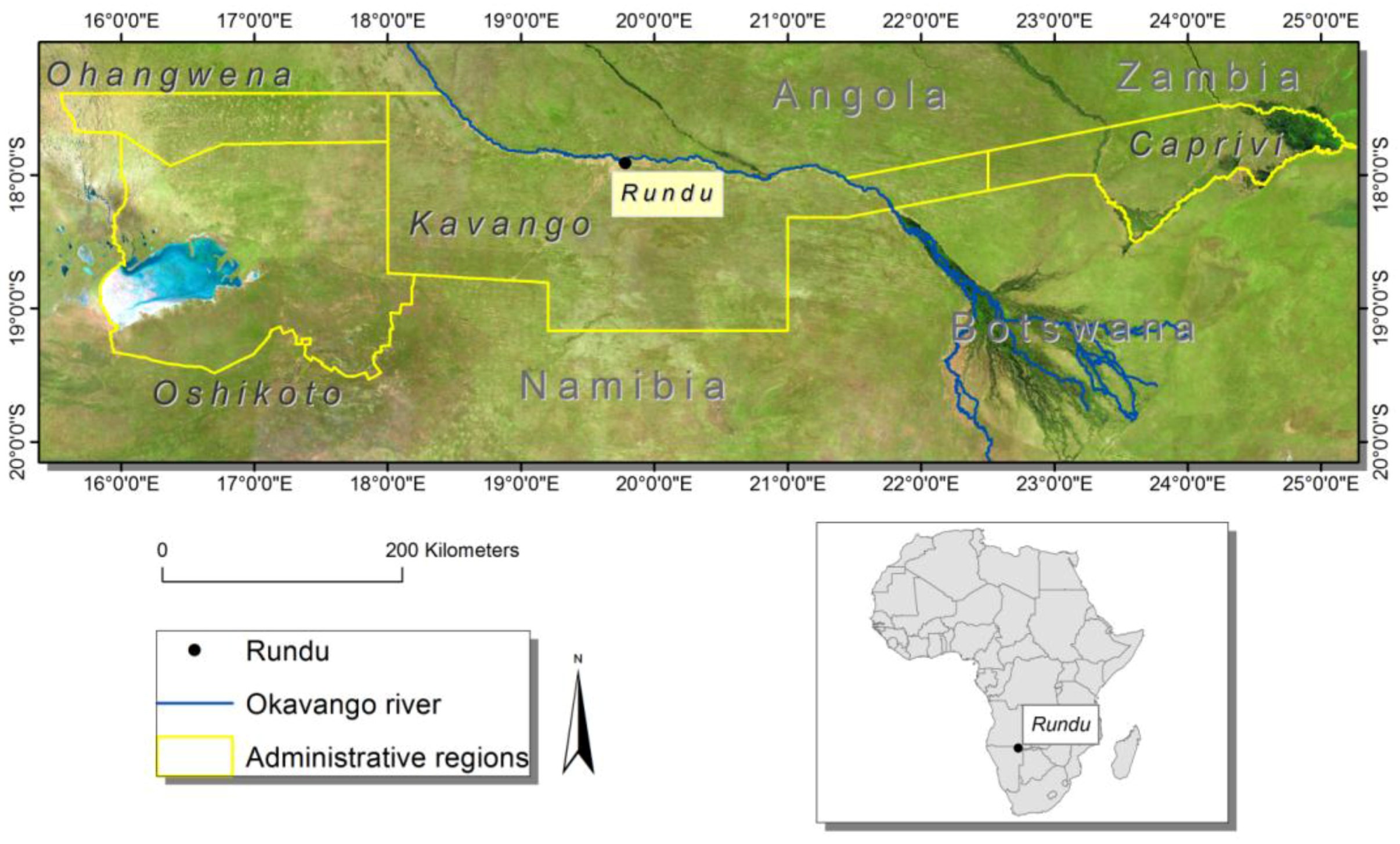
2.1. Study Area
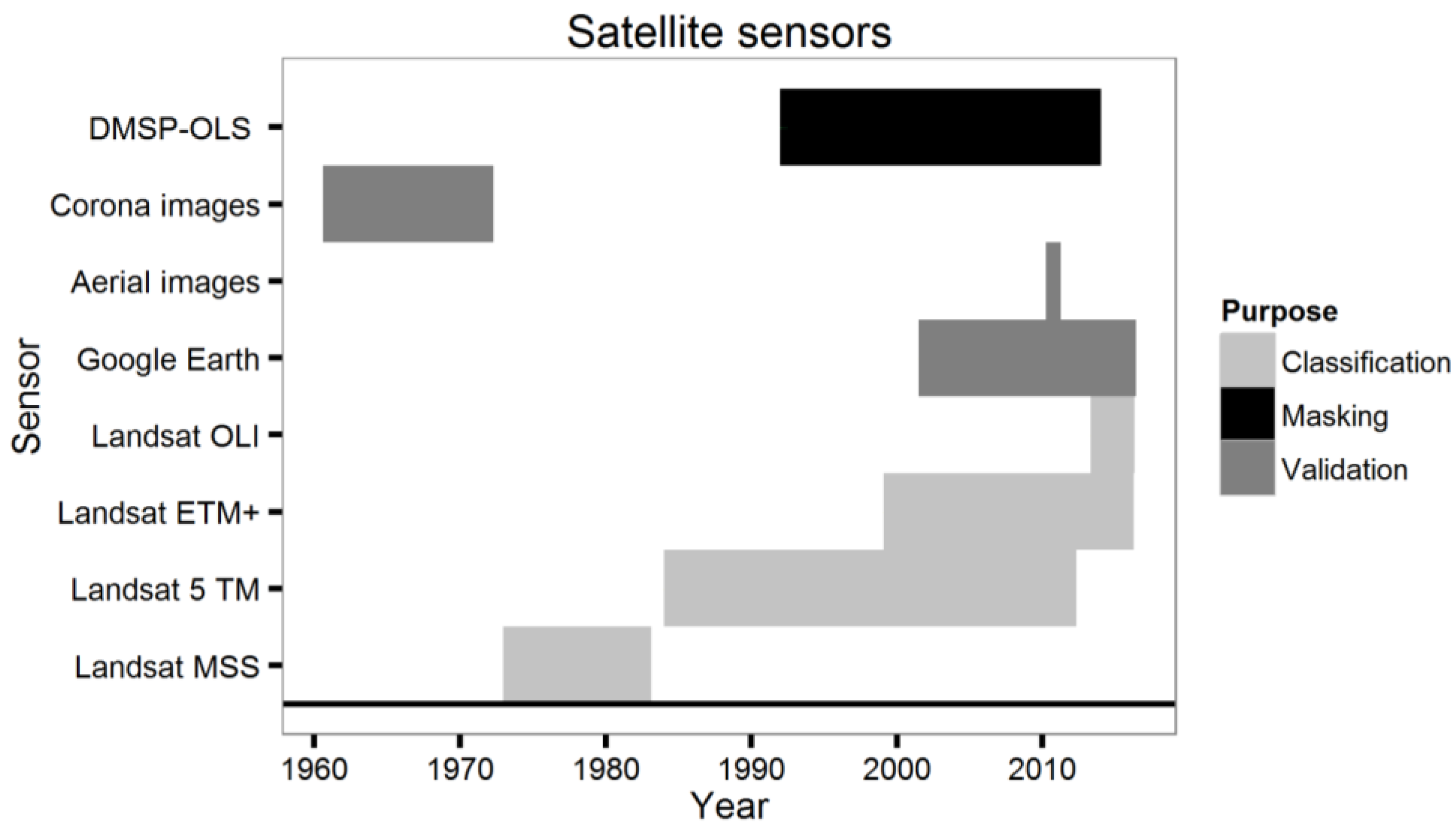
2.2. Landsat Scene Acquisition and Processing
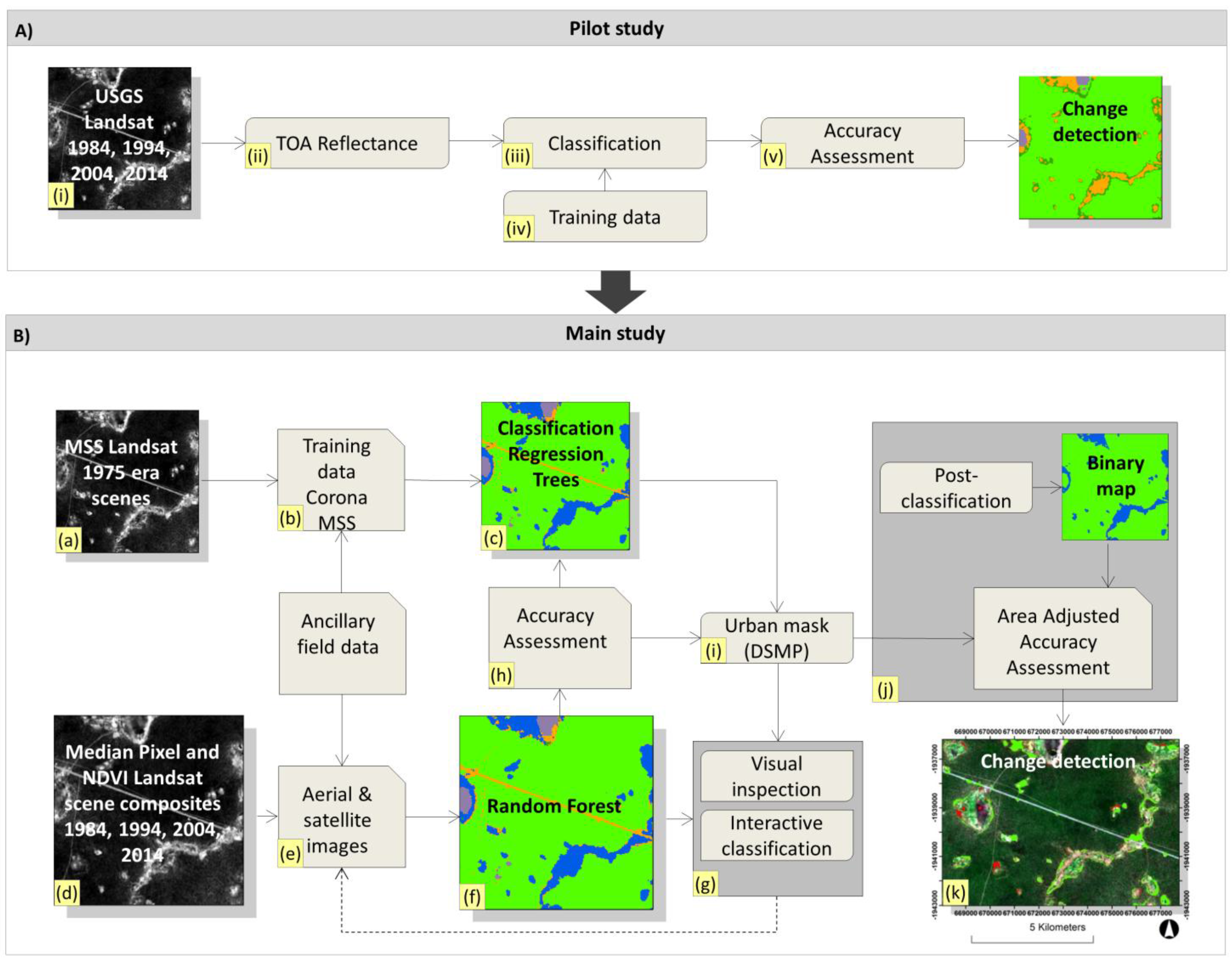
2.3. Classification and Change Detection Work Flow
2.4. Land Cover Change Analysis
2.5. Proximal Variables of Change
2.6. Accuracy Assessment
3. Results and Discussion
3.1. Classification Accuracy
3.2. Limitations
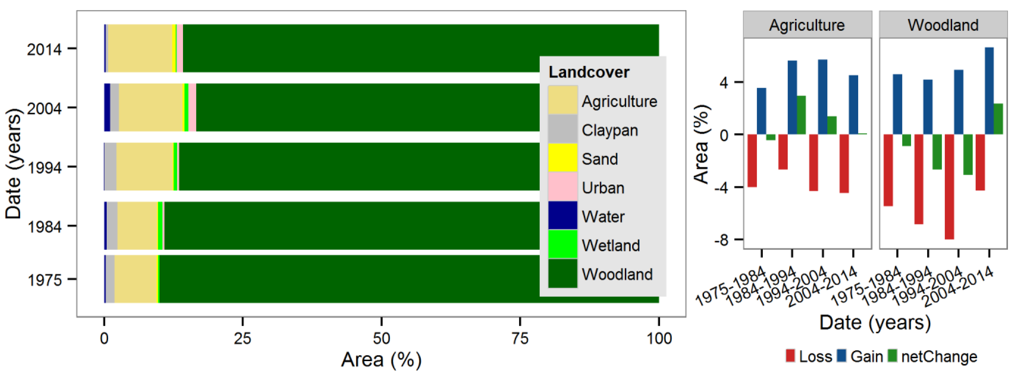
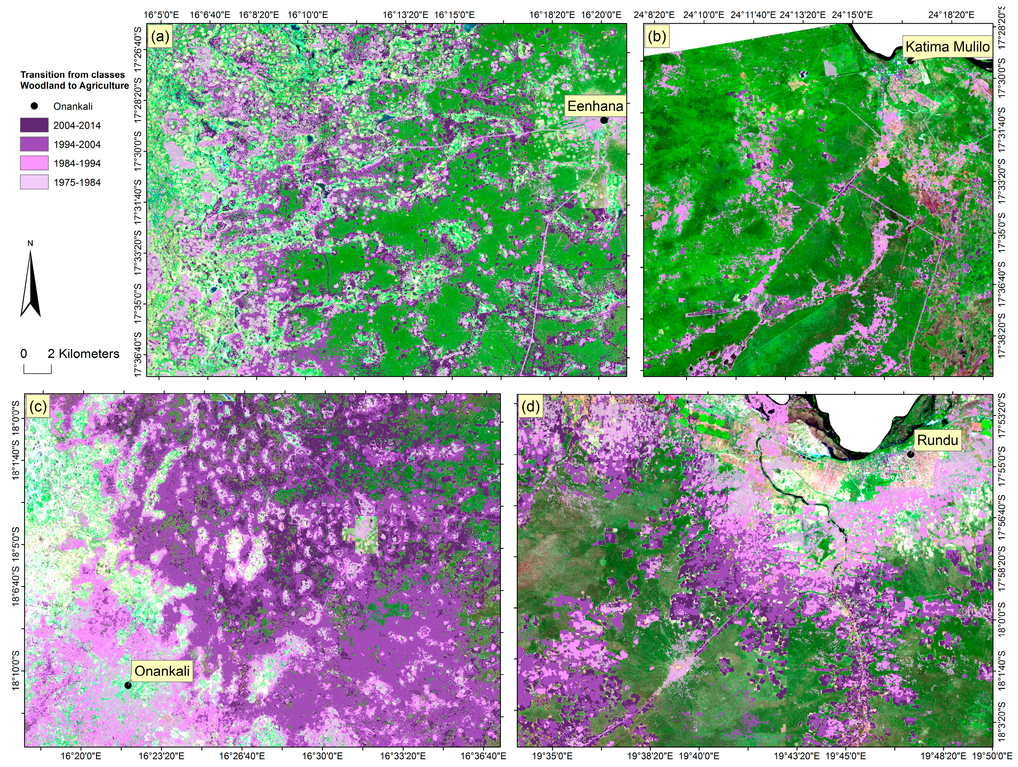
3.3. Change Area, Distribution and Transitions
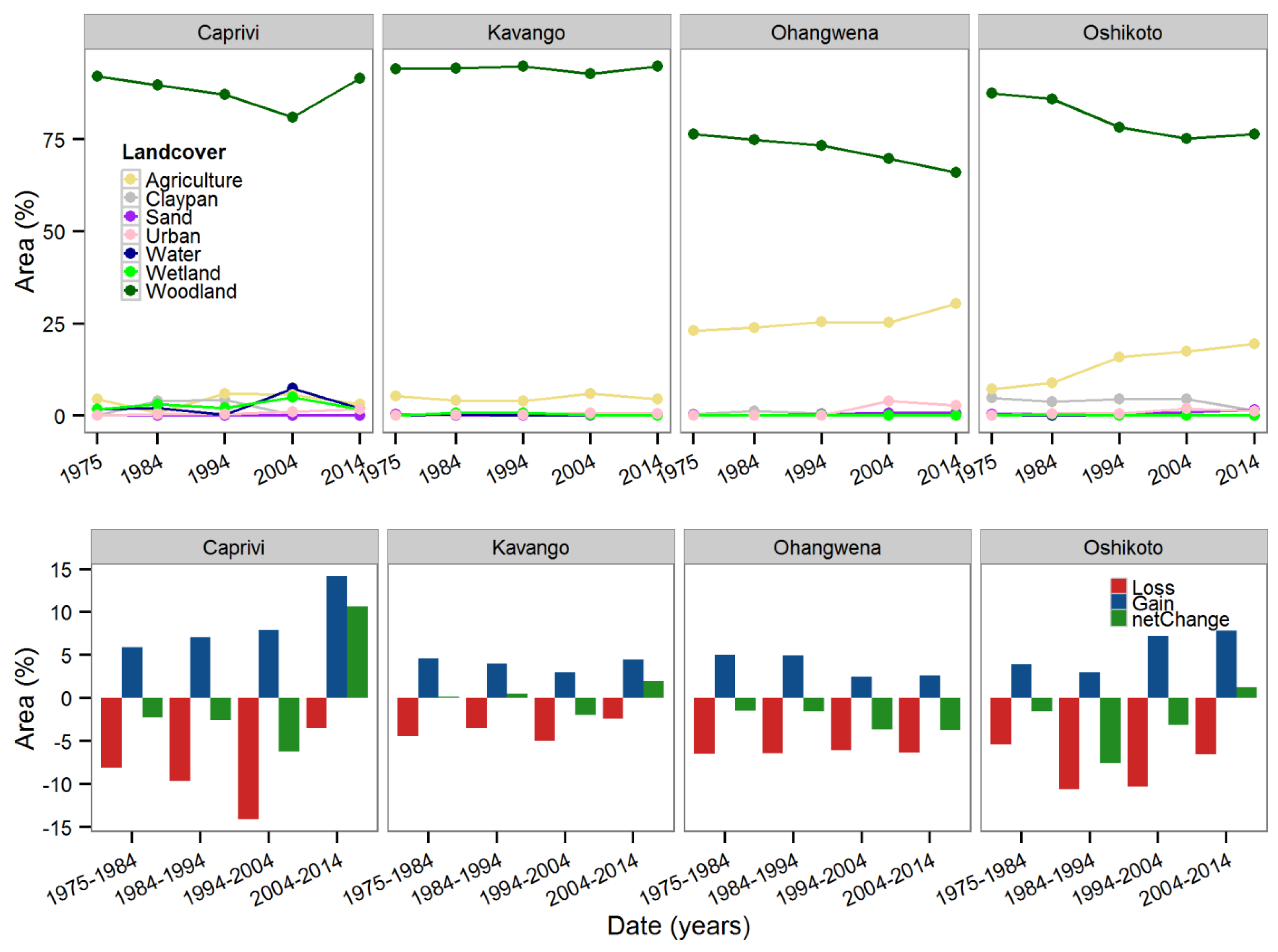
3.4. Land Cover Changes per Administrative Region
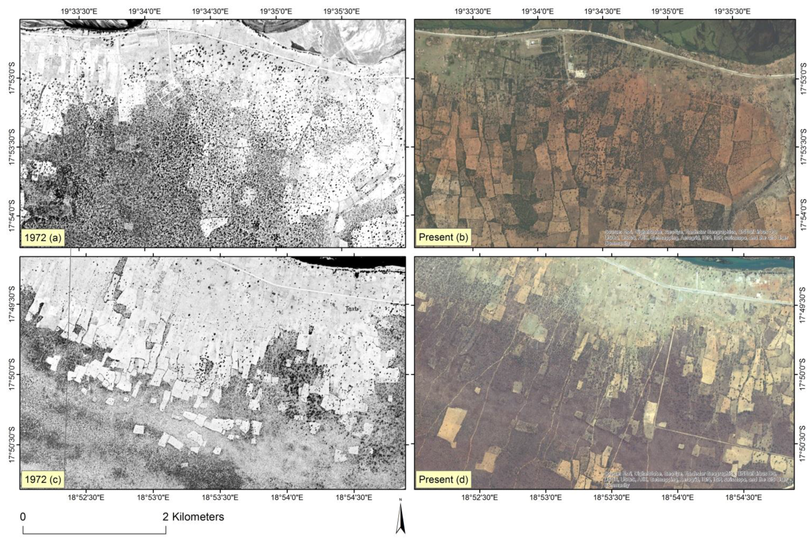
3.5. Drivers, Consequences and Implications of Land Cover Changes
4. Conclusions
Supplementary Materials
Acknowledgments
Author Contributions
Conflicts of Interest
References
- Foley, J.A.; Defries, R.; Asner, G.P.; Barford, C.; Bonan, G.; Carpenter, S.R.; Chapin, F.S.; Coe, M.T.; Daily, G.C.; Gibbs, H.K.; et al. Global consequences of land use. Science 2005, 309, 570–574. [Google Scholar] [CrossRef] [PubMed]
- Tilman, D.; Fargione, J.; Wolff, B.; D’Antonio, C.; Dobson, A.; Howarth, R.; Schindler, D.; Schlesinger, W.H.; Simberloff, D.; Swackhamer, D. Forecasting agriculturally driven global environmental change. Science 2001, 292, 281–284. [Google Scholar] [CrossRef] [PubMed]
- Matson, P.A. Agricultural intensification and ecosystem properties. Science 1997, 277, 504–509. [Google Scholar] [CrossRef] [PubMed]
- Vitousek, P.M.; Mooney, H.A.; Lubchenco, J.; Melillo, J.M. Human domination of Earth’s ecosystems. Science 1997, 277, 494–499. [Google Scholar] [CrossRef]
- DeFries, R.; Achard, F.; Brown, S.; Herold, M.; Murdiyarso, D.; Schlamadinger, B.; de Souza, C. Earth observations for estimating greenhouse gas emissions from deforestation in developing countries. Environ. Sci. Policy 2007, 10, 385–394. [Google Scholar] [CrossRef]
- Ellis, E.C.; Ramankutty, N. Putting people in the map: Anthropogenic biomes of the world. Front. Ecol. Environ. 2008, 6, 439–447. [Google Scholar] [CrossRef]
- DeFries, R.S.; Foley, J.A.; Asner, G.P. Land-use choices: Balancing human needs and ecosystem function. Front. Ecol. Environ. 2004, 2, 249–257. [Google Scholar] [CrossRef]
- Olofsson, P.; Kuemmerle, T.; Griffiths, P.; Knorn, J.; Baccini, A.; Gancz, V.; Blujdea, V.; Houghton, R.A.; Abrudan, I.V.; Woodcock, C.E. Carbon implications of forest restitution in post-socialist Romania. Environ. Res. Lett. 2011, 6, 045202. [Google Scholar] [CrossRef]
- DeFries, R.S.; Houghton, R.A.; Hansen, M.C.; Field, C.B.; Skole, D.; Townshend, J. Carbon emissions from tropical deforestation and regrowth based on satellite observations for the 1980s and 1990s. Proc. Natl. Acad. Sci. USA 2002, 99, 14256–14261. [Google Scholar] [CrossRef] [PubMed]
- Schulz, J.J.; Cayuela, L.; Echeverria, C.; Salas, J.; Rey Benayas, J.M. Monitoring land cover change of the dryland forest landscape of Central Chile (1975–2008). Appl. Geogr. 2010, 30, 436–447. [Google Scholar] [CrossRef]
- Coppin, P.; Jonckheere, I.; Nackaerts, K.; Muys, B.; Lambin, E. Review article digital change detection methods in ecosystem monitoring: A review. Int. J. Remote Sens. 2004, 25, 1565–1596. [Google Scholar] [CrossRef]
- Lu, D.; Mausel, P.; Brondízio, E.; Moran, E. Change detection techniques. Int. J. Remote Sens. 2004, 25, 2365–2401. [Google Scholar] [CrossRef]
- Vittek, M.; Brink, A.; Donnay, F.; Simonetti, D.; Desclée, B. Land cover change monitoring using Landsat MSS/TM satellite image data over West Africa between 1975 and 1990. Remote Sens. 2014, 6, 658–676. [Google Scholar] [CrossRef]
- Baccini, A.; Goetz, S.J.; Walker, W.S.; Laporte, N.T.; Sun, M.; Sulla-Menashe, D.; Hackler, J.; Beck, P.S.A.; Dubayah, R.; Friedl, M.A.; et al. Estimated carbon dioxide emissions from tropical deforestation improved by carbon-density maps. Nat. Clim. Chang. 2012, 2, 182–185. [Google Scholar] [CrossRef]
- Bodart, C.; Brink, A.B.; Donnay, F.; Lupi, A.; Mayaux, P.; Achard, F. Continental estimates of forest cover and forest cover changes in the dry ecosystems of Africa between 1990 and 2000. J. Biogeogr. 2013, 40, 1036–1047. [Google Scholar] [CrossRef] [PubMed]
- UN Food and Agriculture Organisation. Global Forest Resource Assessment; UN Food and Agriculture Organisation: Rome, Italy, 2010. [Google Scholar]
- Erkkilä, A. Living on the land: Change in forest cover in north-central Namibia 1943–1996. Int. J. Afr. Hist. Stud. 2001, 35, 625–626. [Google Scholar]
- Mendelsohn, J.M.; El Obeid, S. Sand and Water: A Profile of the Kavango Region; Struik: Cape Town, South Africa, 2003. [Google Scholar]
- Miles, L.; Newton, A.C.; DeFries, R.S.; Ravilious, C.; May, I.; Blyth, S.; Kapos, V.; Gordon, J.E. A global overview of the conservation status of tropical dry forests. J. Biogeogr. 2006, 33, 491–505. [Google Scholar] [CrossRef]
- Kasperson, R.E.; Archer, E.R. Vulnerable peoples and places. In Ecosystems and Human Well-Being: Current State and Trends: Findings of the Condition and Trends Working Group; Island Press: Washington, DC, USA, 2005; Volume 1, p. 143. [Google Scholar]
- Verlinden, A.; Kruger, A.S. Changing grazing systems in central North Namibia. Land Degrad. Dev. 2007, 18, 179–197. [Google Scholar] [CrossRef]
- Verlinden, A.; Seely, M.K.; Hillyer, A. Settlement, trees and termites in central North Namibia: A case of indigenous resource management. J. Arid Environ. 2006, 66, 307–335. [Google Scholar] [CrossRef]
- Geiss, W. A Preliminary Vegetation Map of Namibia; Namibia Scientific Society: Windhoek, Namibia, 1971. [Google Scholar]
- Scholes, R.; Archer, S. Tree-grass interactions in savannas. Annu. Rev. Ecol. Syst. 1997, 28, 517–544. [Google Scholar] [CrossRef]
- Asner, G.P.; Lobell, D.B. A biogeophysical approach for automated SWIR unmixing of soils and vegetation. Remote Sens. Environ. 2000, 74, 99–112. [Google Scholar] [CrossRef]
- Jung, M.; Henkel, K.; Herold, M.; Churkina, G. Exploiting synergies of global land cover products for carbon cycle modeling. Remote Sens. Environ. 2006, 101, 534–553. [Google Scholar] [CrossRef]
- Herold, M.; Mayaux, P.; Woodcock, C.; Baccini, A.; Schmullius, C. Some challenges in global land cover mapping: An assessment of agreement and accuracy in existing 1 km datasets. Remote Sens. Environ. 2008, 112, 2538–2556. [Google Scholar] [CrossRef]
- Erkkilä, A.; Löfman, S. Forest cover change in the Ohangwena region, northern Namibia: A case study based on multitemporal Landsat images and aerial photography. South. Afr. For. J. 1999, 184, 25–32. [Google Scholar] [CrossRef]
- Röder, A.; Pröpper, M.; Stellmes, M.; Schneibel, A.; Hill, J. Assessing urban growth and rural land use transformations in a cross-border situation in northern Namibia and southern Angola. Land Use Policy 2015, 42, 340–354. [Google Scholar] [CrossRef]
- Pröpper, M.; Gröngröft, A.; Falk, T.; Eschenbach, A.; Fox, T.; Gessner, U.; Hecht, J.; Hinz, M.O.; Huettich, C. Causes and perspectives of land-cover change through expanding cultivation in Kavango. In Biodiversity in Southern Africa. Volume 3: Implications for Landuse and Management; Klaus Hess Publishers: Göttingen, Germany; Windhoek, Namibia, 2010. [Google Scholar]
- Hüttich, C.; Gessner, U.; Herold, M.; Strohbach, B.J.; Schmidt, M.; Keil, M.; Dech, S. On the suitability of MODIS time series metrics to map vegetation types in dry savanna ecosystems: A case study in the Kalahari of NE Namibia. Remote Sens. 2009, 1, 620–643. [Google Scholar] [CrossRef]
- Strohbach, B.J.; Petersen, A. Vegetation of the central Kavango woodlands in Namibia: An example from the mile 46 livestock development centre. S. Afr. J. Bot. 2007, 73, 391–401. [Google Scholar] [CrossRef]
- Verlinden, A.; Laamanen, R. Modelling woody vegetation resources using Landsat TM imagery in northern Namibia. S. Afr. For. J. 2006, 207, 27–39. [Google Scholar]
- Campbell, B.; Angelsen, A.; Cunningham, A.; Katerere, Y.; Sitoe, A.; Wunder, S. Miombo Woodlands—Opportunities and Barriers to Sustainable Forest Management; CIFOR: Bogor, Indonesia, 2007; Available online: http://www.cifor.cgiar.org/miombo/docs/Campbell_BarriersandOpportunities.pdf (accessed on 4 November 2008).
- Wang, L.; D’Odorico, P.; Ringrose, S.; Coetzee, S.; Macko, S.A. Biogeochemistry of Kalahari Sands. J. Arid Environ. 2007, 71, 259–279. [Google Scholar] [CrossRef]
- National Planning Commission. Namibia 2011 Population and Housing Census Preliminary Results; National Planning Commission: Windhoek, Namibia, 2012.
- Verlinden, A.; Dayot, B. A comparison between indigenous environmental knowledge and a conventional vegetation analysis in North Central Namibia. J. Arid Environ. 2005, 62, 143–175. [Google Scholar] [CrossRef]
- Mendelsohn, J.M.; El Obeid, S. Forests and Woodlands of Namibia; RAISON: Windhoek, Namibia, 2005. [Google Scholar]
- Mendelsohn, J.M.; El Obeid, S. The Communal Lands in Eastern Namibia; RAISON: Windhoek, Namibia, 2002. [Google Scholar]
- Verlinden, A.; Laamanen, R. Long term fire scar monitoring with remote sensing in northern Namibia: Relations between fire frequency, rainfall, land cover, fire management and trees. Environ. Monit. Assess. 2006, 112, 231–253. [Google Scholar] [CrossRef] [PubMed]
- United States Geological Survey. Available online: https://www.usgs.gov/ (accessed on 1 June 2014).
- Eastman, J. IDRISI Selva; Clark University: Worcester, MA, USA, 2012. [Google Scholar]
- Google Earth Engine. Available online: https://developers.google.com/earth-engine/ (accessed on 1 June 2014).
- Singh, A. Review article digital change detection techniques using remotely-sensed data. Int. J. Remote Sens. 1989, 10, 989–1003. [Google Scholar] [CrossRef]
- Colwell, J.E.; Weber, F. Forest change detection. In Proceedings of International Symposium on Remote Sensing of Environment, Ann Arbor, MI, USA, 11–15 May 1981; pp. 839–852.
- Gislason, P.O.; Benediktsson, J.A.; Sveinsson, J.R. Random forests for land cover classification. Pattern Recognit. Lett. 2006, 27, 294–300. [Google Scholar] [CrossRef]
- Breiman, L.; Friedman, J.; Stone, C.J.; Olshen, R.A. Classification and Regression Trees; CRC Press: Boca Raton, FL, USA, 1984. [Google Scholar]
- Breiman, L. Random forests. Mach. Learn. 2001, 45, 5–32. [Google Scholar] [CrossRef]
- Elvidge, C.D.; Cinzano, P.; Pettit, D.R.; Arvesen, J.; Sutton, P.; Small, C.; Nemani, R.; Longcore, T.; Rich, C.; Safran, J.; et al. The Nightsat mission concept. Int. J. Remote Sens. 2007, 28, 2645–2670. [Google Scholar] [CrossRef]
- Pontius, R.G.; Shusas, E.; McEachern, M. Detecting important categorical land changes while accounting for persistence. Agric. Ecosyst. Environ. 2004, 101, 251–268. [Google Scholar] [CrossRef]
- Mendelsohn, J. Atlas of Namibia: A Portrait of the Land and Its People; New Africa Books (Pty) Ltd.: Cape Town, South Africa, 2002. [Google Scholar]
- Geist, H.J.; Lambin, E.F. Proximate causes and underlying driving forces of tropical deforestation. BioScience 2002, 52, 143–150. [Google Scholar] [CrossRef]
- Olofsson, P.; Foody, G.M.; Stehman, S.V.; Woodcock, C.E. Making better use of accuracy data in land change studies: Estimating accuracy and area and quantifying uncertainty using stratified estimation. Remote Sens. Environ. 2013, 129, 122–131. [Google Scholar] [CrossRef]
- Shao, G.; Wu, J. On the accuracy of landscape pattern analysis using remote sensing data. Landsc. Ecol. 2008, 23, 505–511. [Google Scholar] [CrossRef]
- Hill, M.J.; Hanan, N.P.; Hoffmann, W.; Scholes, R.; Prince, S.; Ferwerda, J.; Lucas, R.M.; Baker, I.; Arneth, A.; Higgins, S. Remote sensing and modeling of savannas: The state of the dis-union. In Proceedings of the 34th International Symposium on Remote Sensing of the Environment (ISRSE), Sydney, NSW, Australia, 10–15 April 2011.
- Hanan, N.P.; Hill, M.J. Challenges and opportunities for improved remote sensing and modelling of global savannas. In Proceedings of Earth Observation for Land-Atmosphere Interaction Science, Frascati, Italy, 3–5 November 2010.
- Smith, J.H.; Stehman, S.V.; Wickham, J.D.; Yang, L. Effects of landscape characteristics on land-cover class accuracy. Remote Sens. Environ. 2003, 84, 342–349. [Google Scholar] [CrossRef]
- Whiteside, T.G.; Boggs, G.S.; Maier, S.W. Comparing object-based and pixel-based classifications for mapping savannas. Int. J. Appl. Earth Obs. Geoinform. 2011, 13, 884–893. [Google Scholar] [CrossRef]
- Johansen, K.; Arroyo, L.A.; Armston, J.; Phinn, S.; Witte, C. Mapping riparian condition indicators in a sub-tropical savanna environment from discrete return lidar data using object-based image analysis. Ecol. Indic. 2010, 10, 796–807. [Google Scholar] [CrossRef]
- Smith, J.H.; Wickham, J.D.; Stehman, S.V.; Yang, L. Impacts of patch size and land-cover heterogeneity on thematic image classification accuracy. Photogramm. Eng. Remote Sens. 2002, 68, 65–70. [Google Scholar]
- Gessner, U.; Machwitz, M.; Conrad, C.; Dech, S. Estimating the fractional cover of growth forms and bare surface in savannas. A multi-resolution approach based on regression tree ensembles. Remote Sens. Environ. 2013, 129, 90–102. [Google Scholar] [CrossRef]
- Childes, S.L. Phenology of nine common woody species in semi-arid, deciduous Kalahari sand vegetation. Vegetatio 1988, 79, 151–163. [Google Scholar] [CrossRef]
- Vicente-Serrano, S.; Cabello, D.; Tomás-Burguera, M.; Martín-Hernández, N.; Beguería, S.; Azorin-Molina, C.; Kenawy, A. Drought variability and land degradation in semiarid regions: Assessment using remote sensing data and drought indices (1982–2011). Remote Sens. 2015, 7, 4391–4423. [Google Scholar] [CrossRef]
- Asner, G.P.; Elmore, A.J.; Olander, L.P.; Martin, R.E.; Harris, A.T. Grazing systems, ecosystem responses, and global change. Annu. Rev. Environ. Resour. 2004, 29, 261–299. [Google Scholar] [CrossRef]
- Chander, G.; Markham, B.L.; Helder, D.L. Summary of current radiometric calibration coefficients for Landsat MSS, TM, ETM+, and EO-1 ALI sensors. Remote Sens. Environ. 2009, 113, 893–903. [Google Scholar] [CrossRef]
- Ward, D. Do we understand the causes of bush encroachment in African savannas? Afr. J. Range Forage Sci. 2005, 22, 101–105. [Google Scholar] [CrossRef]
- O’Connor, T.G.; Puttick, J.R.; Hoffman, M.T. Bush encroachment in southern Africa: Changes and causes. Afr. J. Range Forage Sci. 2014, 31, 67–88. [Google Scholar] [CrossRef]
- Mitchard, E.T.A.; Flintrop, C.M. Woody encroachment and forest degradation in sub-Saharan Africa’s woodlands and savannas 1982–2006. Philos. Trans. R. Soc. Lond. B Biol. Sci. 2013, 368, 20120406. [Google Scholar] [CrossRef] [PubMed]
- Pimm, S.L.; Jenkins, C.N.; Abell, R.; Brooks, T.M.; Gittleman, J.L.; Joppa, L.N.; Raven, P.H.; Roberts, C.M.; Sexton, J.O. The biodiversity of species and their rates of extinction, distribution, and protection. Science 2014, 344, 1246752. [Google Scholar] [CrossRef] [PubMed]
- Szantoi, Z.; Brink, A.; Buchanan, G.; Bastin, L.; Lupi, A.; Simonetti, D.; Mayaux, P.; Peedell, S.; Davy, J. A simple remote sensing based information system for monitoring sites of conservation importance. Remote Sens. Ecol. Conserv. 2016, 2, 16–24. [Google Scholar] [CrossRef]
- Malan, J. Guide to the Communal Land Reform Act, 2002; Land, Environment, and Development Project, Legal Assistance Centre, and the Advocacy Unit, Namibia National Farmers’ Union: Windhoek, Namibia, 2009. [Google Scholar]
- Mendelsohn, J. Farming Systems in Namibia; Research & Information Services of Namibia: Windhoek, Namibia, 2006. [Google Scholar]
- Gröngröft, A.; Luther-Mosebach, J.; Landschreiber, L.; Eschenbach, A. Mashare soils. Biodivers. Ecol. 2013, 5, 105–108. [Google Scholar] [CrossRef]
- Oldeland, J.; Erb, C.; Finck, M.; Jürgens, N. Environmental Assessments in the Okavango Region; BEE, Biocentre Klein Flottbek and Botanical Garden, University of Hamburg: Hamburg, Germany, 2013. [Google Scholar]
- Hansen, M.C.; Potapov, P.V.; Moore, R.; Hancher, M.; Turubanova, S.A.; Tyukavina, A.; Thau, D.; Stehman, S.V.; Goetz, S.J.; Loveland, T.R.; et al. High-resolution global maps of 21st-century forest cover change. Science 2013, 342, 850–853. [Google Scholar] [CrossRef] [PubMed]
- Mendelsohn, J. Customary and Legislative Aspects of Land Registration and Management on Communal Land in Namibia; Ministry of Land and Resettlement and European Union: Windhoek, Namibia, 2008.
- Zahabu, E.; Skutsch, M.M.; Sosovele, H.; Malimbwi, R.E. Reduced emissions from deforestation and degradation. Afr. J. Ecol. 2007, 45, 451–453. [Google Scholar] [CrossRef]
- Jindal, R.; Swallow, B.; Kerr, J. Forestry-based carbon sequestration projects in Africa: Potential benefits and challenges. Nat. Resour. Forum 2008, 32, 116–130. [Google Scholar] [CrossRef]
- Bond, I.; Chambwera, M.; Jones, B.; Chundama, M.; Nhantumbo, I. REDD+ in Dryland Forests Issues and Prospects for Pro-Poor REDD in the Miombo Woodlands of Southern Africa; International Institute for Environment and Development (UK): London, UK, 2010. [Google Scholar]
- Chidumayo, E.N.; Gumbo, D.J. The Dry Forests and Woodlands of Africa: Managing for Products and Services; Earthscan: London, UK, 2010. [Google Scholar]
- Drusch, M.; Del Bello, U.; Carlier, S.; Colin, O.; Fernandez, V.; Gascon, F.; Hoersch, B.; Isola, C.; Laberinti, P.; Martimort, P. Sentinel-2: ESA’s optical high-resolution mission for GMES operational services. Remote Sens. Environ. 2012, 120, 25–36. [Google Scholar] [CrossRef]
- Kuenzer, C.; Dech, S.; Wagner, W. Remote sensing time series revealing land surface dynamics: Status quo and the pathway ahead. In Remote Sensing Time Series; Springer: Basel, Switzerland, 2015; pp. 1–24. [Google Scholar]
- Pettorelli, N.; Vik, J.O.; Mysterud, A.; Gaillard, J.M.; Tucker, C.J.; Stenseth, N.C. Using the satellite-derived NDVI to assess ecological responses to environmental change. Trends Ecol. Evol. 2005, 20, 503–510. [Google Scholar] [CrossRef] [PubMed]


| Class | Description |
|---|---|
| Water | Rivers, lakes and standing water bodies |
| Clay pan | Dry lake bed; layer of clay alternating with water during the wet season |
| Agriculture | Arable cropland, orchards and pasture, villages and farmsteads |
| Bare ground | Exposed sands, beaches, riparian sand bars, dunes and roads |
| Woodland | Predominant land cover class; includes all savannah woodland transitions |
| Wetland | Seasonally flooded areas found adjacent to rivers and lakes |
| Urban | Densely populated areas, paved roads, concrete, warehouses, and tarmac (masked) |
| Date | Change Estimate (km2) | Error (km2) | Actual Change (km2) |
|---|---|---|---|
| 1975–1984 | 577 | 20 | 5906 |
| 1984–1994 | 2161 | 159 | 7411 |
| 1994–2004 | 678 | 300 | 8653 |
| 2004–2014 | 1556 | 76 | 4624 |
© 2016 by the authors; licensee MDPI, Basel, Switzerland. This article is an open access article distributed under the terms and conditions of the Creative Commons Attribution (CC-BY) license (http://creativecommons.org/licenses/by/4.0/).
Share and Cite
Wingate, V.R.; Phinn, S.R.; Kuhn, N.; Bloemertz, L.; Dhanjal-Adams, K.L. Mapping Decadal Land Cover Changes in the Woodlands of North Eastern Namibia from 1975 to 2014 Using the Landsat Satellite Archived Data. Remote Sens. 2016, 8, 681. https://doi.org/10.3390/rs8080681
Wingate VR, Phinn SR, Kuhn N, Bloemertz L, Dhanjal-Adams KL. Mapping Decadal Land Cover Changes in the Woodlands of North Eastern Namibia from 1975 to 2014 Using the Landsat Satellite Archived Data. Remote Sensing. 2016; 8(8):681. https://doi.org/10.3390/rs8080681
Chicago/Turabian StyleWingate, Vladimir R., Stuart R. Phinn, Nikolaus Kuhn, Lena Bloemertz, and Kiran L. Dhanjal-Adams. 2016. "Mapping Decadal Land Cover Changes in the Woodlands of North Eastern Namibia from 1975 to 2014 Using the Landsat Satellite Archived Data" Remote Sensing 8, no. 8: 681. https://doi.org/10.3390/rs8080681
APA StyleWingate, V. R., Phinn, S. R., Kuhn, N., Bloemertz, L., & Dhanjal-Adams, K. L. (2016). Mapping Decadal Land Cover Changes in the Woodlands of North Eastern Namibia from 1975 to 2014 Using the Landsat Satellite Archived Data. Remote Sensing, 8(8), 681. https://doi.org/10.3390/rs8080681