Article

Estimating Understory Temperatures Using MODIS LST in Mixed Cordilleran Forests

1
Department of Geography, University of Calgary, Calgary, AB T2N 1N4, Canada
2
Department of Renewable Resources, University of Alberta, Edmonton, AB T6G 2H1, Canada
*
Author to whom correspondence should be addressed.
Remote Sens. 2016, 8(8), 658; https://doi.org/10.3390/rs8080658
Submission received: 26 April 2016 / Revised: 19 July 2016 / Accepted: 9 August 2016 / Published: 15 August 2016

Abstract

:
Satellite remote sensing provides a rapid and broad-scale means for monitoring vegetation phenology and its relationship with fluctuations in air temperature. Investigating the response of plant communities to climate change is needed to gain insight into the potentially detrimental effects on ecosystem processes. While many studies have used satellite-derived land surface temperature (LST) as a proxy for air temperature, few studies have attempted to create and validate models of forest understory temperature (Tust), as it is obscured from these space-borne observations. This study worked to predict instantaneous values of Tust using daily Moderate Resolution Imaging Spectroradiometer (MODIS) LST data over a 99,000 km2 study area located in the Rocky Mountains of western Alberta, Canada. Specifically, we aimed to identify the forest characteristics that improve estimates of Tust over using LST alone. Our top model predicted Tust to within a mean absolute error (MAE) of 1.4 °C with an overall model fit of R2 = 0.89 over two growing seasons. Canopy closure and the LiDAR-derived standard deviation of canopy height metric were found to significantly improve estimations of Tust over MODIS LST alone. These findings demonstrate that canopy structure and forest stand-type function to differentiate understory air temperatures from ambient canopy temperature as seen by the sensor overhead.

Graphical Abstract

1. Introduction

There is growing interest in using remote sensing for observing Earth’s microclimates in order to acquire a better understanding of ecosystem functions such as vegetation phenology, carbon flux, and the timing of species trophic interactions (e.g., [1]). Surface air temperature (Tair) is a critical driver of these environmental processes, especially at high latitudes where seasonal transitions are more highly pronounced [2]. However, obtaining reliable measurements of Tair across the landscape is often hindered by missing values due to gaps in the data [3]. These voids are typically a result of the limited density of meteorological stations distributed across the landscape [4]. Spatial interpolation of these data is prone to error because of the distance and fine-scale temperature aberrations between stations, especially in mountainous areas where their distribution tends to be even sparser [5,6,7]. Remote sensing of land surface temperature (LST) helps to resolve this issue by providing an inherently spatialized gridded surface that covers even the most remote regions. The Moderate Resolution Imaging Spectroradiometer (MODIS) has proven invaluable for monitoring year-round global temperature in high temporal detail [8]. MODIS LST data is particularly popular because of its high level of post-processing which produces accuracies of ≤1 °C [9]. MODIS LST has successfully been used to predict Tair (e.g., [10,11]), however Tair recordings are commonly made in open areas or high above the forest canopy from eddy covariance flux towers (e.g., [12,13]). With observations at heights in excess of 30 m, the relationship between MODIS LST and air temperature in the understory (Tust) is relatively unknown.
Radiometers do not measure air temperature directly, rather the LST estimations are obtained through a split-window algorithm which translates thermal infrared (TIR) observations into skin temperature of the observable land surfaces (i.e., bare land, urban areas, forest canopy) [14]. LST is quite different from Tair and they do not generally correlate well [15]. This relationship is improved over vegetated areas, since emitted radiance is affected by surface type [16]. There is a simple and physical relationship between fractional vegetation cover and thermal properties detected by the sensor [17]. The disparity between LST and Tair is greater over areas of exposed soil and other surfaces with low emittance [18]. As a result, the direct relationship between LST and Tair needs to be determined using a supplementary estimation technique.
Variable forest cover types introduce additional complexities by creating irregularities in the latent heat flux and other radiative exchanges [19,20]. The prevalent methodologies used to parameterize Tair from LST include (i) physical models of the surface energy balance; and (ii) the temperature–vegetation index (TVX) method [21]. Energy-balance models are based on physical processes, and require large amounts of radiation and latent heat flux data typically not provided by remote-sensing techniques [15,22]. The spectral information obtained by the sensor is not able to perceive many of these complex physical variables, such as wind speed and soil moisture [23].
The challenge in measuring the processes that govern Tair above vegetation leave most models under-parameterized, and this is the main reason for the development of the temperature–vegetation index (TVX) method [17]. The premise of the TVX method is an established linear and negative correlation between a remotely-sensed vegetation index, often the normalized difference vegetation index (NDVI), and satellite-derived LST [24,25]. The TVX assumes that the radiometric temperature of a fully vegetated canopy is in equilibrium with Tair [26]. The premise is that dense vegetation radiates heat so efficiently that it remains close in temperature to the surrounding ambient air [18]. In effect, the assumption is that the top-of-canopy temperature is the same as the canopy itself [11]. How this assumption translates to estimating understory temperatures, and the relationship with MODIS LST across different vegetative strata, requires further investigation.
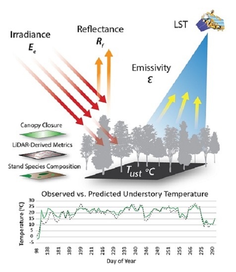
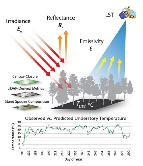
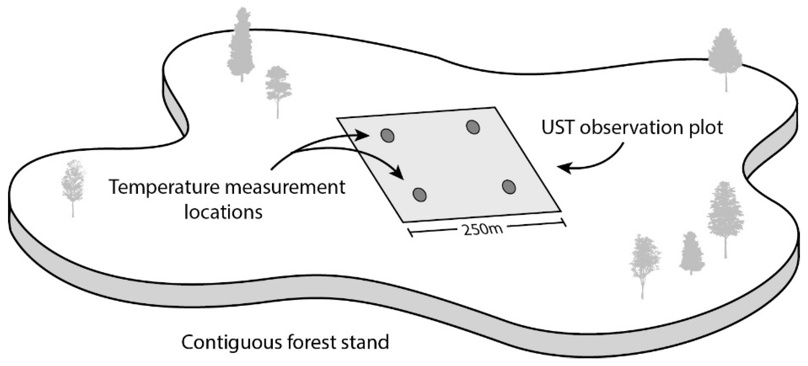
The difference between air temperatures above and below the forest canopy is generally a result of near-surface environmental lapse rates and distance from the ground [1]. The perspective of forests from a space-borne sensor is of the top of the canopy, and the thermal information beneath is hidden from view due to the relative opacity of the forest itself. The boundary layer separating the emissive properties of the understory and the supracanopy air mass is occupied by different types and densities of canopy vegetation. Therefore estimations of 
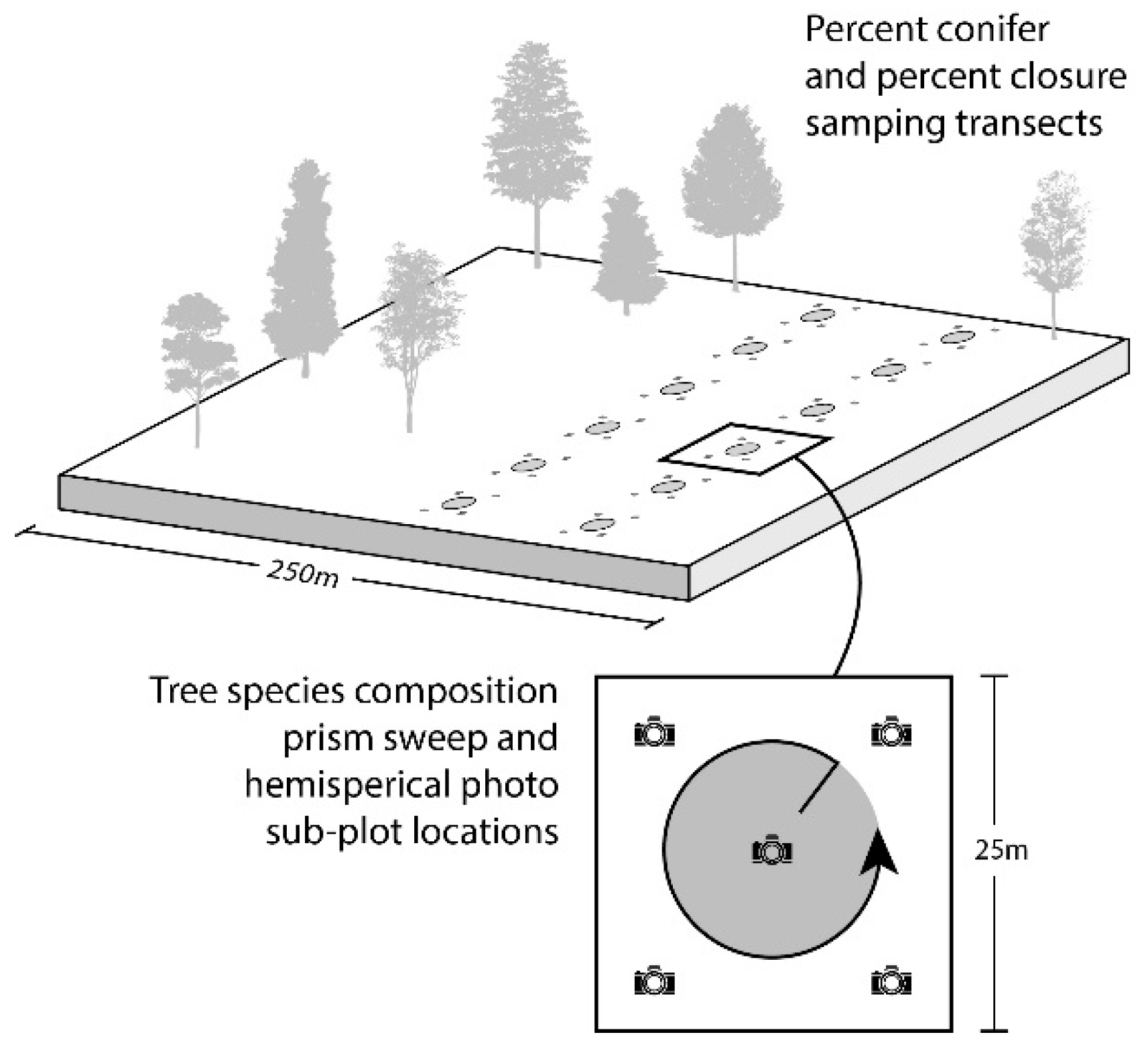
Tust, without assuming that it is in equilibrium with the canopy, should incorporate physical characteristics of the canopy in addition to MODIS LST. These characteristics can be acquired in a number of ways. Traditionally, forest attributes have been obtained through mensuration techniques developed by the timber industry [27]. Metrics such as tree height, diameter, and canopy closure are generally used to estimate the volume of harvestable timber in a stand. These methods have since been adapted to characterize forest landscapes for ecosystem management and studies of species ecology (e.g., [28]). Recently, these conventional mensuration practices have been complemented by the development of airborne laser scanning (LiDAR) data. LiDAR systems procure detailed models of vegetation in three dimensions, with the fundamental benefit of penetrating the canopy to extract additional information from the understory [29,30]. Most of the existing literature emphasizes characteristics of the overstory, with relatively few papers using LiDAR to examine the understory within an ecological context [31,32,33]. Nijland et al. [34] compared LiDAR-derived canopy metrics with more conventional climate and land cover based variables to model the distribution of various understory species with mixed success.
The importance of estimating understory temperature is to increase our understanding of its cause–effect relationship with other natural processes. For example, the timing of phenological events is closely linked to changes in ambient temperature, where the life histories of many species are explicitly adapted to the seasonal environments in which they live [35]. Monitoring microclimate dynamics provides insight into species sensitivities to weather anomalies and global trends in temperature from climate change [36,37]. The MODIS LST imagery offers a mechanism to observe this significant driver of ecosystem dynamics over the broad scale, which in turn provides maps as a basis for species conservation, habitat management, or identifying additional environmental responses to climate change [38,39,40,41]. The present effort to model Tust is motivated by our involvement in an ongoing grizzly bear (Ursus arctos) research program where we are working to monitor critical habitat for this threatened species in Alberta, Canada [42]. These animals strategically exploit a wide variety of understory plants that provide variable nutrition at differential times of the growing season [43]. The eventual goal is to model the bears’ response to shifting understory phenology by mapping Tust accumulations, or growing degree days (GDD) (e.g., [44,45,46]).
The objective of this study is to predict instantaneous measurements of Tust using daily MODIS LST data and a combination of LiDAR-derived canopy metrics and conventional forest inventory variables. Although MODIS LST has been previously correlated with Tair [47,48,49], estimating Tust has not been studied in detail. There is also an absence of in situ meteorological data measured at comparable resolutions to the remotely sensed imagery with which it is correlated [1]. Using a multivariate statistical approach, we ranked the comparative importance of LiDAR and conventional forest inventory variables in estimating instantaneous 
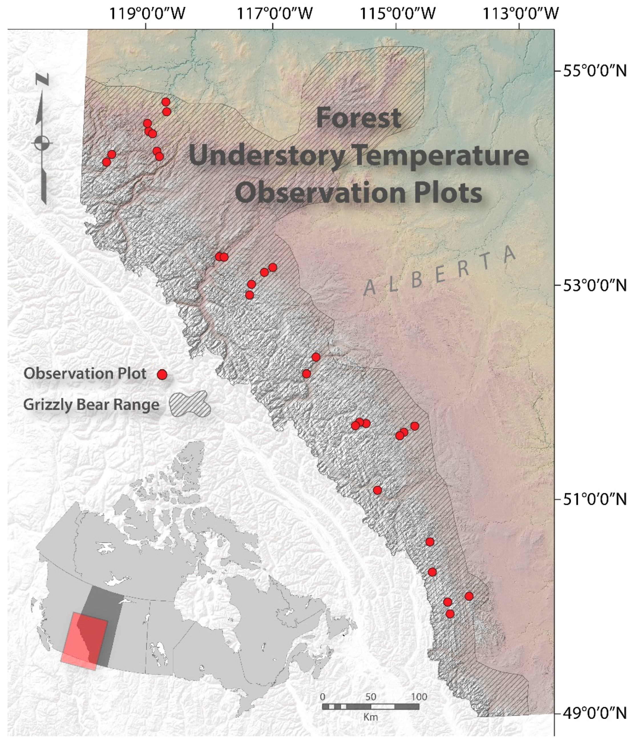
Tust at the MODIS pixel-scale. In situ Tust measurements were collected over two seasons using a widespread network of meteorological stations distributed throughout the foothills and Rocky Mountains of western Alberta, Canada. Although it is normally assumed that the vegetated canopy is the same temperature as the surrounding ambient air [18,26], the understory will experience dissimilar temperatures as a result of the general moderating effect of the canopy [50]. We hypothesized that based on the interactions between MODIS LST and forest canopies [16], that supplementary forest canopy and stand variables would significantly improve model predictions of Tust over those made by LST alone.

2. Materials and Methods

2.1. Study Area

The study area extends over 700 km along the eastern slopes of the Alberta Rocky Mountains (49°N to 55°N) in western Canada (Figure 1). Tust observation plots were placed at near-regular latitudinal intervals along elevational transects covering a gradient from 800 m to 1800 m. The forests of the region are typified by deciduous trembling aspen (Populus tremuloides) and balsam poplar (Populus balsamifera) in mixed stands with white spruce (Picea glauca) at lower elevations. The mountains are dominated by mature conifer forests of lodgepole pine (Pinus contorta) and Engelmann spruce (Picea engelmannii). Stand composition of the observation plots ranged from 40% being purely coniferous, 40% mixed, and 20% entirely deciduous.

2.2. In Situ Tust Observations

Within the study area, twenty-nine broadly dispersed Tust observation plots were selected to obtain a range of temperature regimes, forest composition types, and variability in canopy closure. Each plot was 250 × 250 m (62,500 m2) in size and located within comparatively homogenous forest stands that extended a minimum of 250 m beyond the edges of the plot. This spatial buffer retained representative temperatures for that particular stand type, minimizing the influence from surrounding divergent cover types. This stand size also corresponds with the areal unit scale of a 1 km MODIS LST pixel (Figure 2). Within each plot, four meteorological sensors recorded 8-bit hourly temperature from early spring (pre green-up) until after autumn senescence for two growing seasons: 2011 and 2012. The sensors were enclosed in solar radiation shields 1 m above ground-level, approximating the typical height of shrubby understory vegetation.

2.3. MODIS Land Surface Temperature Observations

The daily LST product is collected by the sun-synchronous, near-polar orbiting Terra (MOD11A1) and Aqua (MYD11A1) satellites, with Aqua in an ascending orbit and Terra in a descending orbit, having two daily equatorial crossings each at 13:30, 01:30, and 10:30, 22:30, respectively (local solar time) [51]. LST is derived from the MODIS thermal emissivity band channels 31 (10.78–11.28 μm) and 32 (11.77–12.27 μm). Atmospheric effects are corrected using a split-window algorithm that compares the differential thermal radiation absorption between these two bands [52]. Version v005 was the most up-to-date MODIS LST product available, with an accuracy of ≤1°K, and provided significantly improved spatial coverage, stability, and accuracy compared to previous versions [9,47]. Data download and processing was automated using R programming language [53]. The tiled daily LST data were obtained from the NASA Land Processes Distributed Active Archive Center (LP DAAC) for all dates corresponding with the in situ Tust observations. The MODIS Reprojection Tool [54] was used to reproject the MOD11A1, MYD11A1, and coincident local solar view time products from Sinusoidal to 1 km gridded geotiff’s in Universal Transverse Mercator projection (UTM Zone 11N, NAD83 datum) using nearest-neighbor resampling. Pixel values were then rescaled and converted to degrees Celsius. An abridged methodology is shown in Figure 3.
Accurate LST measurements are highly dependent on the amount of cloud cover at the time of overpass, therefore a two-step filter process was adapted from Neteler [6] and Zorer et al. [46] to obtain only the highest quality pixels for each observation plot. The first step used the integrated image bitword quality assessment (QA) flags to mask out cloud or corrupted image pixels. Data were selected with “0” flags in each quality control field, e.g., 00 in “Mandatory QA flags”, 00 in “Data quality flag”, average emissivity error ≤0.01, average LST error ≤1°K, and view-angle less than 40 degrees from nadir [55]. The second step involved a 1 km proximity search around each observation plot pixel, considering that cloud-contaminated pixels not detected by the QA flags most commonly occur along the edges of clouds [6,56]. Any adjacent pixel with more than a 5°K difference from an observation plot pixel was considered corrupted (i.e., from vapor or cloud shadow) and not used in the model. Overall, 1920 MODIS LST images were processed.
To obtain instantaneous measurements of in situ Tust, temporally linking observations with coincident MODIS LST view times was critical. This procedure can be problematic, considering MOD11A1 and MYD11A1 tile data can contain a mosaic of non-sequential and temporally unrelated surface temperatures resulting from multiple daily imaging from adjacent swaths [48]. Off-nadir viewing is performed to maximize the amount of cloud-free ground surface visible to the sensor during each orbit. To separate the image in to spatially corrected view times, a longitudinal correction was made for each plot and the equation of time (1) was applied to the image solar view times to yield local view times (±30 s) with corrections for daylight savings (2) [57].
Equation of Time = 0.258(COSx) − 7.416(SINx) − 3.648(COS2x) − 9.228(SIN2x)
where the angle x is defined as a function of the day of year and produces the difference between mean solar time and true solar time on a given date.
L o c a l   V i e w   T i m e   =   t s E O T 60   +   L C   ± D a y l i g h t   S a v i n g
where ts is solar time, EOT is the equation of time, and LC is the site longitudinal correction from the nearest standard meridian. Once calculated, local LST view times were then rounded to the nearest hour and coupled with the corresponding hourly Tust plot measurement for every clear sky observation during the study period.

2.4. LiDAR-Derived Canopy Metrics

Airborne laser scanning data for the study area were provided by the Government of Alberta’s Forest Management Branch. The data were collected between 2003 and 2010 (although the majority is circa 2007 during predominantly leaf-on conditions) using sensors capable of detecting four returns per pulse. Data densities were typically 1–2 returns/m2. The LiDAR data were normalized to height above ground-level and processed into a suite of height and structure metrics using standard processing routines available in FUSION [58]. The majority of metrics used first returns in accordance with recommendations in Bater et al. [59], who found that first-return vegetation-height metrics were more stable than those calculated from all-pulse returns. The canopy metrics were averaged over the entire 250 m study plot to approach the areal-unit scale of the MODIS imagery.
Individual LiDAR-derived metrics were selected for use in the models based on their most plausible and intrinsic role in explaining the Tust/LST interface, and also on their predictive success in previous structural understory LiDAR models (e.g., [34]) (Table 1). For example, the ratio pa14 is considered a proxy for canopy closure (1.4 m being the understory height threshold [60]), while standard deviation of canopy height (stdd) can be thought of as absolute vegetation roughness [61]. A number of indices were included because they incorporate all pulse returns. Although being less stable, they potentially provide more information on subcanopies and understory vegetation than metrics derived from first returns alone [62]. This was an effort to maximize the utility of the LiDAR data, as it only provides information on vegetation structure, with no additional nuanced ecological information on species assemblies and abundance.

2.5. Conventional Forest and Topographic Variables

Before the widespread availability of LiDAR and optical remote sensing, forest structure and compositional characteristics were (and still are) traditionally collected by personnel on the ground [27]. These ground data, combined with LST and derived topographic variables, have provided suitable model results for estimating Tair. For example, Parmentier et al. [20] used a number of covariates such as forest land cover type, elevation, and aspect to predict monthly average Tair to approximately 2.5 °C. Variables representing land cover and vegetation type are particularly important since they affect surface emissivity [14]. Differences between AM and PM LST values have been found to vary between 0.3 °C to 3.2 °C depending on cover type [63]. Taking into consideration this sensitivity of LST to land cover and canopy density, forest tree species composition (percent conifer) in each of the 29 observation plots was measured every 50 m along two 250 m stratified-random linear transects (14 subplots per plot). A representative sample of tree species was obtained using a 360° sweep of each subplot using a wedge prism relascope (Figure 4). Canopy closure was measured during leaf-on conditions using five hemispherical photographs at each subplot and later processed with WinSCANOPY software [64] to calculate percent closure. Increased closure was assumed to have insulative properties that provide thermal cover for the ambient understory air mass [16,65].
A 10 m photogrammetrically compiled digital elevation model was used to extract topographic variables including elevation, slope, aspect, and annual terrain solar radiation in watt-hours per square meter (WH/m2) using ArcGIS 10.3 software [66]. Throughout the year the difference between same-day AM and PM LST observations can vary up to 5 °C [63]. Because of this, Julian day was included in the models to account for this variability in the surface energy balance at different times of the growing season. Benali et al. [47] found Julian day to have little predictive effect in their Tair models, so the quadratic polynomial of Julian day was used in this study to better represent the seasonal temperature curve (Table 2).

2.6. Statistical Methods and Model Ranking

Regression approaches have previously demonstrated accurate predictions of Tair using solely LST or LST associated with ancillary variables [4,13,46,49,67]. In this application, models were divided into three groupings similar to the organization used by Benali et al. [47], where they modeled instantaneous MODIS LST observations during the (i) daytime; (ii) night; and (iii) using both datasets combined (hereafter referred to as the daytime, night, and day–night models). Separating the dataset in this manner was intended to isolate any effect from differing diurnal near-surface temperature gradients, insolation variability during the day, and outgoing radiation at night. Within the view-time groupings, candidate models were organized into subgroupings established on explanatory variable type (conventional variables, LiDAR-derived metrics, and both types combined) to assess any marked improvement in model performance between them. Generalized linear models were derived in STATA 13 statistical software [68] to estimate instantaneous values of Tust. Random effects (GLS estimator) were used to offset bias from using multiple temperature observations within single sites. A cross-correlation between explanatory variables tested for both linear and monotonic relationships to ensure no collinearity within models. Akaike information criterion (AIC) was used to perform rankings of the candidate models. This procedure seeks to find a balance between model fit (log likelihood) and the number of variables in the model, penalizing those with too much complexity, ranking the best-fit and most parsimonious model as the highest [69]. A total of 4153 day and night clear-sky observations were made during the study period (Figure 5); 20% of these data were randomly withheld for validation [70].

3. Results

The quadratic function of Julian day and LST was set as the standard null model, as these two variables were found to explain more than 80% of the variability in Tust. Julian day explained 20% more variability than LST alone, which is considered good for ecological phenomena [71]. Using all clear-sky observations, separate baseline model rankings of the two variable types (conventional and LiDAR-derived) was performed to get an overview of their relative importance in predicting Tust (Table 3). The delta AIC (Δi) is a measure of each model relative to the top-ranked model, where the criterion suggests substantial evidence for models within Δi < 2. Values between 3 and 7 indicate that the model has considerably less support, and Δi > 10 indicates that the model is very unlikely [72]. Akaike weights (wi) can be interpreted as the probability that the top-ranked model is the best in the set of candidate models [69,73]. Of the conventional metrics, the best model was explained (in addition to the null) by the interaction between LST and percent conifer, which describes the proportion of coniferous trees within a sample unit. The effect of the interaction term in the model can be interpreted as a linkage between these two variables where the influence of forest composition on Tust depends on the coincident LST value at the time of observation. Without the interaction, we are simply trying to predict Tust as solely the unique effect of percent conifer. The top two conventional metric models lead the rankings, each having Akaike weights of 0.50 (percent conifer and the interaction of LST with percent conifer). There was weak support for the addition of elevation, since it is equally ranked with the percent conifer interaction model despite increasing model complexity. By and large, employing conventional variables imparts a major improvement in estimating Tust over using LST alone, which was ranked very poorly.
There was no observed improvement in the prediction of Tust using exclusively LiDAR-derived metrics over the null model (Table 3). The best-performing was skewness, although there is some optimism in the strength of the other LiDAR models since they are all within 2 AIC values of the top ranked model (the null). Any LiDAR-derived metric model containing an interaction term had significantly reduced performance which was reflected by a large increase in AIC value.
The overall top-ranked models from the final groupings (conventional, LiDAR-derived, and both combined) were directly compared to gauge which supplementary variable type best predicts Tust. This comparison was performed for each overpass dataset (daytime, night, and day–night). The combination of conventional variables and LiDAR-derived metrics clearly produced the best models, regardless of view time, as reflected by the large Akaike weights (Table 4).
Percent canopy closure (cc) and the LiDAR-derived metric standard deviation of canopy height (stdd) both appear in all of the top-ranked models. They are often in the form of an interaction term with LST, which is a strong indication of an interrelationship with the forest canopy. At night, the standardized coefficients show that for every percent increase in canopy closure, there will be a 0.06 °C increase in Tust (Table 5). During the day, for every unit increase in closure, Tust decreases 0.12 °C. Also in the top daytime models was the percent returns above 1.4 m (pa14) metric, which is the LiDAR-derived equivalent to canopy closure. This metric had a similar negative daytime influence as closure, where an increase in this variable produces a slight drop in Tust. For both the daytime and day–night models, the interaction term of the LiDAR-derived standard deviation of canopy height was positive, and implies that when LST interacts with increasingly rough canopies, Tust increases, but very little. At night this relationship is inverted, and a higher standard deviation in height results in a cooling of Tust. The percent conifer coefficient was negative, suggesting that as the percentage of conifers increases, Tust will decrease. Overall, canopy closure and the standard deviation of canopy height were the most influential ancillary variables for estimating Tust.
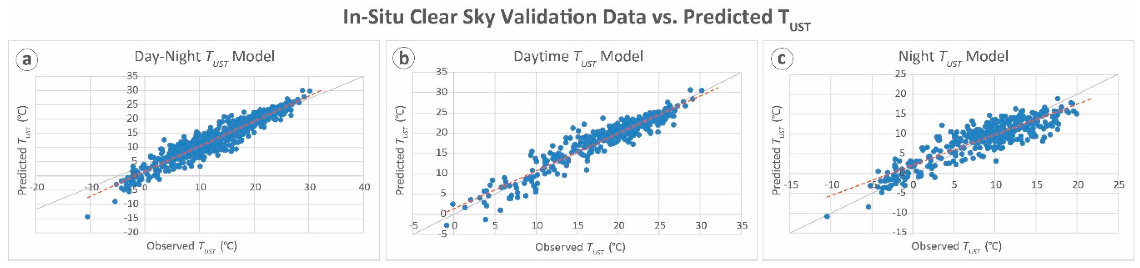
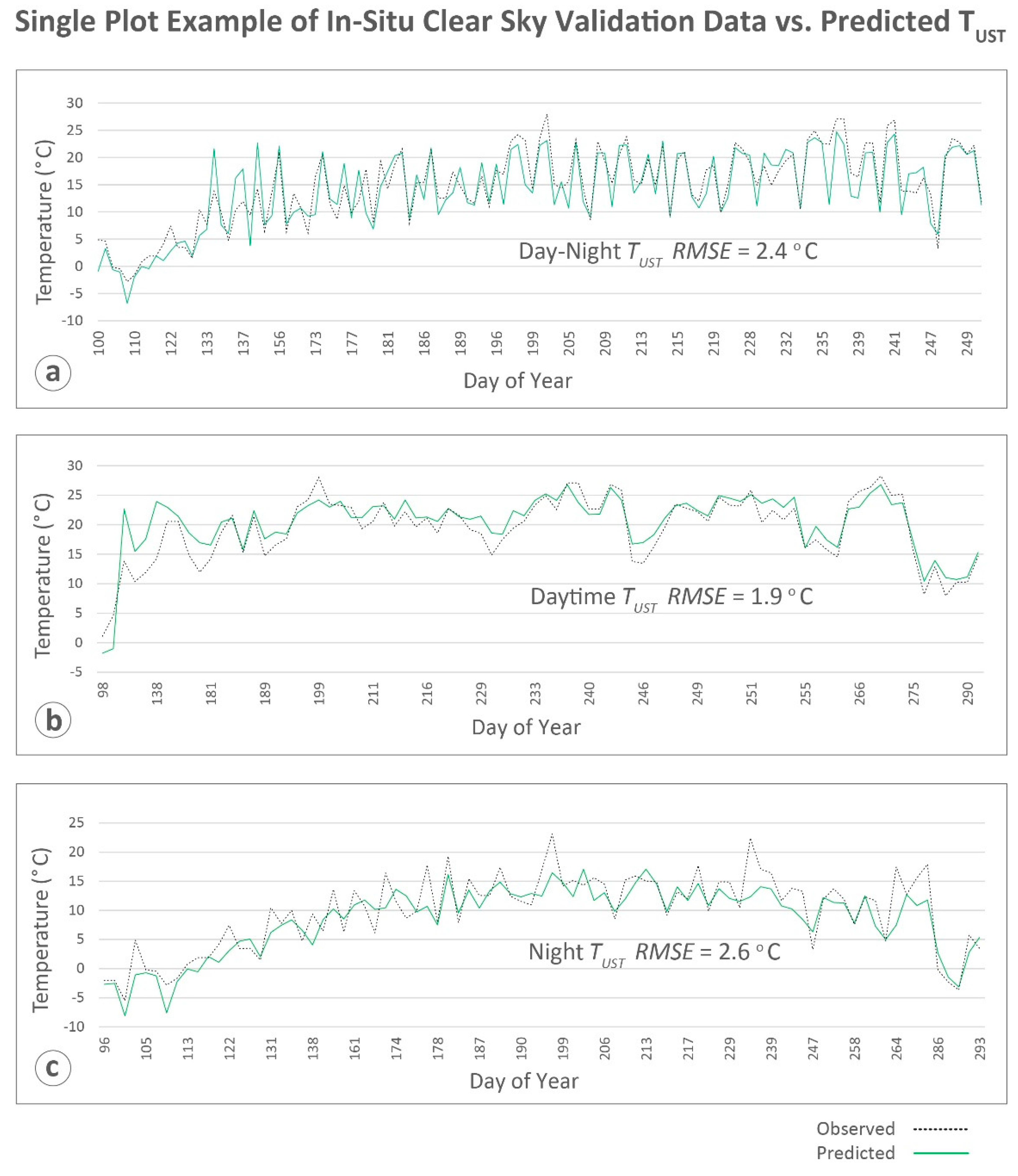
The daytime model was the best performing overall, with a model fit of R2 = 0.89, and the lowest validation error of mean absolute error (MAE) = 1.4 °C. This prediction accuracy parallels estimations of Tair [4,13,49], which is noteworthy considering the predictions are of temperatures beneath the forest canopy (Table 6; Figure 6).
The best day–night model had the same model fit as the daytime model (R2 = 0.89), but had a 0.5 °C increase in error (MAE of 1.9 °C). Although this model had no overall bias, the validation data show a slight Tust underprediction in cooler temperatures that occur during the very start and end of the growing season (Figure 7). The top model derived from night observations had the lowest model fit of the three MODIS view times (R2 = 0.77) and a small error increase over the daytime model in estimation error (MAE = 2.1 °C). The model appears to underestimate higher temperatures and overestimate colder temperatures which seem to balance out, producing no predictive bias on average.

4. Discussion

Forest type, density, and canopy structure all have an impact on the relationship between MODIS LST and understory air temperature. In this paper, we examined which metrics coupled with MODIS LST improve estimates of Tust. This is, to our knowledge, the first study of its kind to specifically model air temperatures in the understory using MODIS LST. We statistically predicted instantaneous values of Tust at a 250 m plot-scale to within MAE 1.4 °C–2.1 °C (depending on the time of day). This is comparable to previous canopy-top Tair models that had error ranging from 1.3 °C to 3.5 °C and similar model fit [4,10,13,47]. The fit slightly exceeded that obtained by Hanes and Schwartz [1], who modeled maximum daily Tair at the base of a flux tower (1.5 m) (R2 = 0.86).
The Tust estimates were consistently accurate over a range of forest types and densities. This may be a result of the overall effectiveness of the model variables at representing the forest canopy characteristics. This variability could not be explained by LST alone (null model) as demonstrated in the AIC rankings. Despite the cost of increased model complexity, those which contained canopy metrics consistently ranked higher than the LST null model. A likelihood ratio test was performed to determine if these top-ranked models estimated Tust significantly better than the null. The results found that the addition of canopy metrics produce a significant improvement over the LST null in the day–night combined model (p < 0.001), and marginally significant in the daytime and night models (p = 0.08; p = 0.07).
The improvement of the models through the addition of the canopy metrics implies that there is a distinction between canopy-top (Tair) and understory temperatures. The difference is likely a result of moderation from the canopy [50,74]. Hanes and Schwartz found that as canopy vegetation becomes increasingly dense during spring leaf out, MODIS LST values begin to approach air temperatures at 1.5 m above ground. In areas where canopy density is reduced, the influence of the overlying forest is diminished and therefore LST should deviate from Tair. However, the Tust estimates across the study area are consistently accurate despite the broad range of forest densities in the plots (10%–70% closure). This finding implies that, unlike Tair, the relationship between LST and Tust is likely consistent regardless of canopy closure.
Modeling day and night LST as separate datasets highlighted daytime as the optimal diurnal period to observe Tust. The daytime model was best overall, with a 10% increase in model fit and 0.7 °C lower error than at night. The majority of previous Tair studies (e.g., [12]) have found increased accuracy during the night, which is attributed to less interference from reflected daytime radiation [75]. The improved daytime accuracy in the Tust models may be owed to modeling entirely within forested sites and the inherent difference of estimating Tust as opposed to Tair. Essentially, the radiative exchanges in the understory are sufficiently unique to those above the canopy resulting in improved daytime Tust observations. In addition, the predominance of conifer trees in the study area may have augmented the performance of the daytime model, since low albedo coniferous canopy absorbs and emits energy more effectively than deciduous [76]; green-needle forest is considered a near-perfect emitter of thermal radiation [77]. This is supported in a daytime model by the positive interaction between LST and percent conifer. This same interaction term is not present in the night model, perhaps because there is no potential for interaction with sunlight.
Conifer forests are also drier than deciduous, ultimately affecting the latent heat flux between them throughout the diurnal cycle. Williamson et al. [48] and Niclòs et al. [4] found that soil moisture was a significant predictor of Tair as it affects surface emissivity. Considering at-site soil moisture was not measured in this study, GIS-derived variables could have been used as proxies for moisture such as a wet area map [34]. Cresswell et al. [78] explain that since the Earth’s skin surface temperature is generally higher than Tair during the day and cooler at night, this will lead to overestimation and underestimation of air temperature in diurnal Tair models, respectively. However, this estimation bias was not observed between the Tust models, perhaps from the moderating effect of the canopy. At night, there was a positive LST interaction with canopy closure which in turn increased Tust. During the day, this relationship was negative and for every percent increase in closure, Tust decreased 0.12 °C. These results corroborate that the canopy shades the understory during the day and insulates it at night [33,79]. This also implies that the understory microclimate is unique to the overlying canopy and therefore emphasizes the distinction between Tair and Tust.
Regarding the performance of the LiDAR-derived metrics, they contributed to all of the top-ranked models, indicating some overall utility. The standard deviation of canopy height was the most predictive either as a solitary variable (at night) or interacting with LST (daytime). It would be more intuitive that average height or canopy density (percent returns above 1.4 m) should explain more variability in Tust; rather it was the roughness of the forest as expressed by the standard deviation of height [33]. During the daytime Tust rises when forest structure becomes increasingly rough, while at night the opposite occurs, where a higher standard deviation results in lower Tust. A rough surface would be characteristic of forest with a strong variation in age structure or disturbance patterns such as trails or cut lines. Although not in the top-ranked models, LiDAR-derived skewness in the distribution of tree heights appeared strongly in many of the models, having a significant yet subtle influence on Tust. Skewness is a similar metric to standard deviation and signifies canopy complexities resulting from variable age structure or directional trends in height across the plot due to soil conditions or slope [80]. The correlation of this metric with Tust was at all times negative, suggesting that as skewness in height increases, Tust drops slightly. The relative contribution to model improvement using the LiDAR metrics raises the question of the advantage of these data over the conventional and GIS-derived variables. Ultimately, it depends on the scale and objectives of the research; in this Tust analysis, the benefits of the LiDAR metrics were not as substantial as the conventional variables. Conversely, the cost of traditional ground measurements are considerably more than LiDAR surveys [81], especially in contrast to the increasing availability of LiDAR technology and platforms such as unmanned aerial systems [82,83].
Downscaling the 2-pulse-per-meter LiDAR metrics to the 250 m plot-scale could have impacted their effectiveness as explanatory variables of Tust. This was done to match the areal unit scale of the observation plots, however it is unlikely that the effect was significant as averaging would only remove the extreme and outlying values. Tompalski et al. [84] compared stand-level LiDAR estimates of tree volume to individual volume measurements and found them to be very similar. The areal scale of 250 m was conceivably an improvement over point-source temperature measurements made by lone meteorological stations or flux towers. The relatively low root mean square error (RMSE) in the Tust models may be indicative of measuring in situ temperature at a broader 250 m scale instead of discrete points on the landscape. The observation plots were located in the center of more expansive areas of homogeneous forest as a solution to the disparity between the resolutions of the larger MODIS LST pixel and the Tust plots. Olsson and Jonsson [85] found that different scales of gridded temperature source-data (e.g., MODIS LST) had no significant influence on the accuracy of their forest phenology models.
For this mitigation approach to operate effectively, it was assumed that temperature across the broader homogenous stand was uniform. This assumption was validated over two seasons, by recording in situ air temperature within a 250 m plot placed at the center of a broad expanse (2700 km2) of perfectly homogenous land cover (native grassland). Employing the identical methodologies as in the forested plots, these data were used to train the LST null model. Air temperature estimates in the validation plot had an average RMSE increase of 2 °C over the equivalent null model estimates in the forested plots. Theoretically, the error should have been lower since the validation plot had completely uniform land cover relative to the principal observation plots. However, this result substantiates that forest cover improves statistical estimates of air temperature using LST [22].
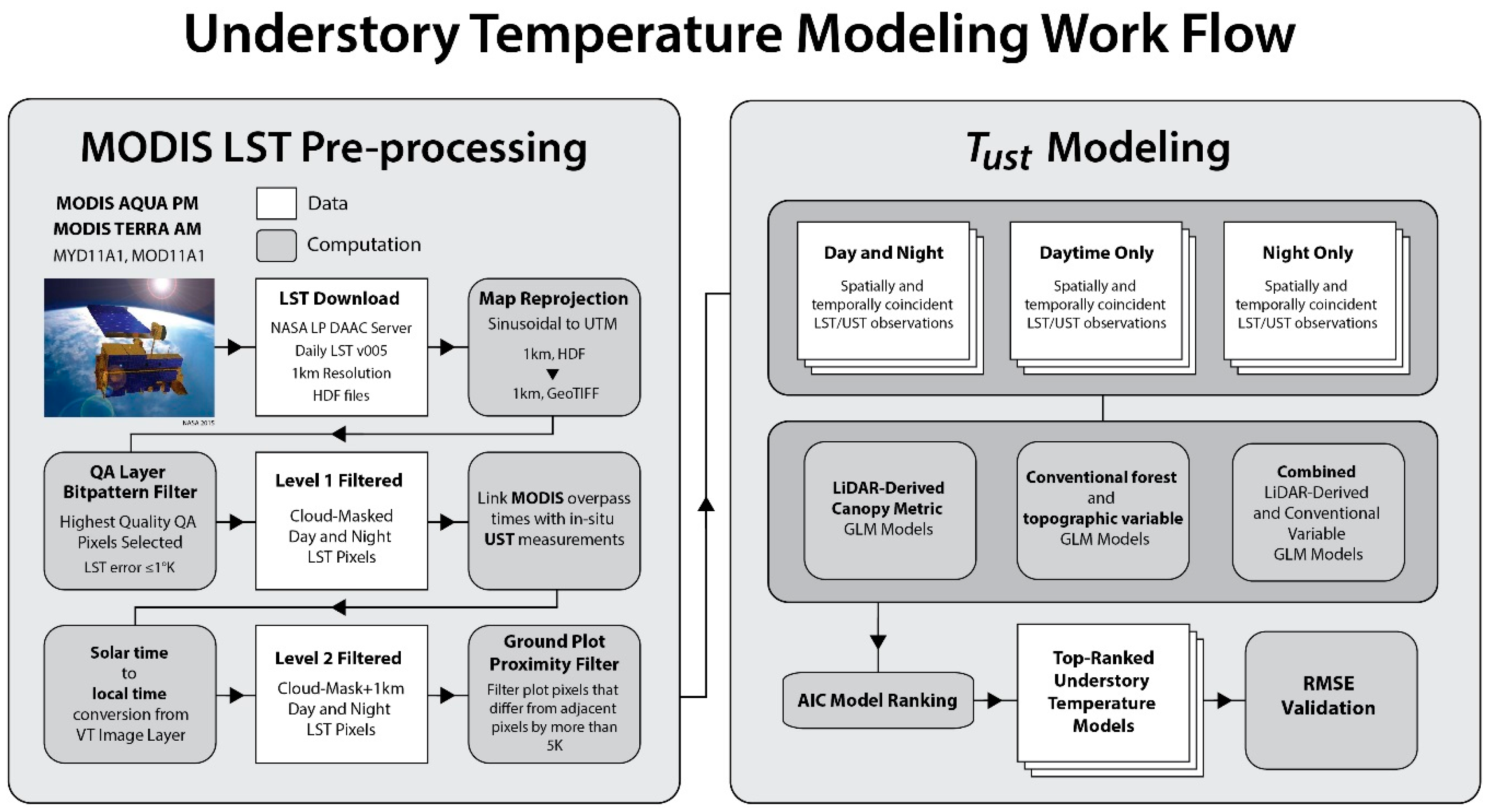
The tiled and projected M*D11A1 products were chosen for this study based on their ease of use and successful application in previous models (e.g., [6,46]). The lower-level LST swath data are less modified and unaffected by projection error or temporal adjustments. However, opting for the higher-level product was a tradeoff between these errors versus the benefit of having the obvious cloud-contaminated LST values removed. During pre-processing the LST imagery selected for this study was reprojected and resampled, which introduces geometric error: chiefly the potential to alter the LST pixel value with values from adjacent cover types. We attempted to mitigate this issue by working in forest stands that were much larger than the plots in which observations were made. Some error may have originated from intrinsic uncertainties in the radiometric or geometric precision of the original MODIS LST data [6], yet this was mitigated by using only the highest quality QA filtered pixels for the analysis. The local time correction made during pre-processing produced times that were truly instantaneous or within 30 min of a MODIS overpass. It is unlikely that this period was sufficient to allow any significant change in temperature on the ground, but it cannot be ruled out completely.
Terrain complexity within the study area introduced an assortment topographic and microclimatic factors, but these had little effect on the model results. This was expected since this study was a within-pixel analysis with no broader spatial interpolation. Observation plots with limited topography were intentionally selected as “targets” for MODIS in an attempt to constrain the variability of Tust solely to forest type and structure. Elevation was the only significant topographic variable in the models because small differences in elevation produce considerable changes in the environmental lapse rate (e.g., [7]). The use of aspirated solar radiation shields worked to limit in situ Tust measurement bias. However, variability in canopy cover between plots may have exposed some sensors to slightly more radiation than others, potentially altering the results [86].
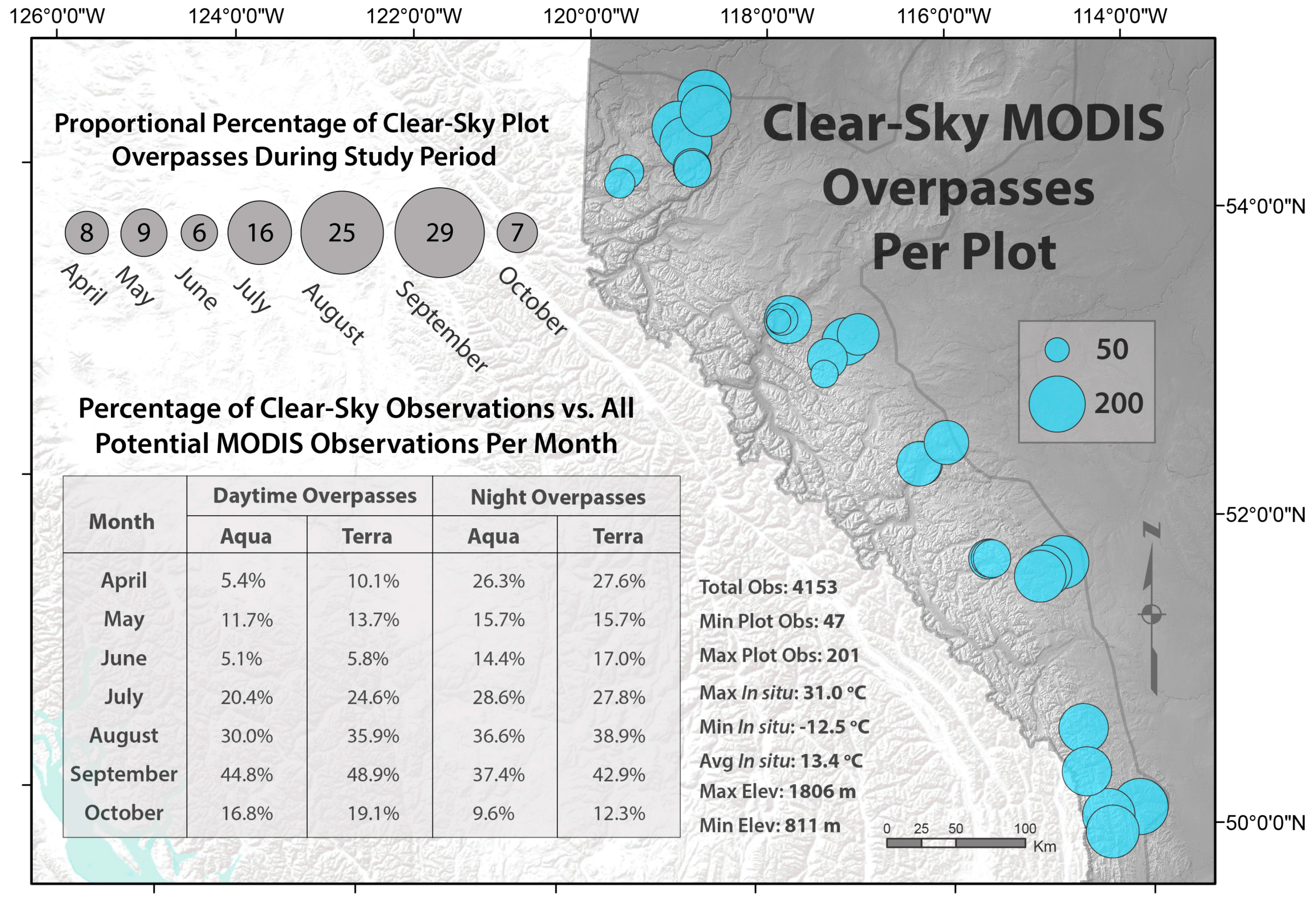
Clear-sky overpasses occurred predominantly during the summer and autumn months, however a considerable proportion occurred in autumn. The canopy is mostly intact for the first half of September, but leaf senescence may have introduced some bias in the small proportion of plots that were deciduous. Given the enduring issue of cloud over the mountains, there was a tradeoff between increased observations during a reliably clear time of year and the transition in canopy attributes. An extended observation period was required to observe the full phenological progression of the understory and to obtain a range of seasonal temperatures. Other sources of model uncertainty most likely occurred during exceedingly cold times of year. The MODIS LST product is accurate to ±1 °C between the temperatures of −10 °C and 50 °C [9], there were early and late season temperatures during the study period that were approximately −20 °C potentially reducing model accuracy. This evidence of seasonal variability affecting model estimates is substantiated by Hanes and Schwartz [1] who found that differences between Tair and MODIS LST are increasingly divergent during colder parts of the year in temperate climates, mainly due to snow cover. However, for the purposes of using Tust for monitoring vegetation phenology, the accuracy of Tust models is not critical during these colder periods since the plants are still dormant and GDD accumulations have not yet begun.
Overall, the models demonstrate that estimates of Tust using MODIS LST can be refined with additional variables which characterize the interface between the top of the forest canopy and the understory. These results facilitate the next step in this research to monitor understory phenology over the entire study area. This requires spatially extending the models beyond the observation plots across the gridded MODIS LST surface to produce maps of daily Tust. GDD maps derived from Tust should provide improved accuracy in predictions of understory plant phenology than those derived from canopy-top Tair. Hanes and Schwartz [1] found that top-of-flux tower GDD accumulations underpredicted plant phenology opposed to measurements made closer to the ground since lapse rates produce cooler temperatures at height. The instantaneous Tust models derived in this study will ultimately facilitate the development of improved land surface phenology maps.

5. Conclusions

Fluctuations in surface air temperature drive a variety of environmental processes which include radiative energy and gas fluxes, species interactions, and vegetation growth. Recently there has been growing importance on collecting thermal data from satellite platforms to estimate Tair at regional and global extents [16,87]. However, the use of remote sensing for modeling forest understory temperatures has yet to be explored. In this paper we described a methodology for predicting plot-scale Tust using MODIS LST and a combination of conventional forest inventory variables and LiDAR-derived canopy metrics. The objective aimed to identify which of these ancillary characteristics played a critical role in modifying estimates of the underlying temperatures. Tust was predicted to within 1.4 °C across a variety of forest types and elevations. Canopy closure and the LiDAR-derived standard deviation of canopy height metric were found to significantly improve estimations of Tust over MODIS LST alone. These findings confirm that canopy structure and forest stand-type can function to differentiate understory air temperatures from ambient canopy temperature as observed by the sensor overhead.
This study developed a remote sensing procedure that works to uncover detailed microclimatic conditions beneath the forest canopy. This type of mechanistic data is particularly useful for ecological modeling [88], but is normally obtained from solitary weather stations or gridded top-of-canopy temperature surfaces. The Tust models were trained using in situ temperature data collected over a broader ground surface to approximate the pixel size of the MODIS imagery. This effort to align the spatial scale of observations likely improved the results and is recommended for any remote sensing investigations collecting surface temperature at moderate resolutions.
These models provide useful estimations of Tust at the plot-scale, but to fully benefit from the spatial nature of the remotely-sensed datasets it would be essential to develop broad-extent daily maps of Tust. There is a need for such a dataset, but foreseeable challenges include producing maps without spatial or temporal punctuations in the time series. Current trends in global climate necessitate predictions of how ecosystem processes will respond to these changes [89,90], and continuous maps of air temperature are instrumental in answering this question. Future research in this area promises to be rewarding as space-borne technologies continuously advance alongside ongoing LST product improvements (e.g., the recent release of MODIS collection version 6). These invaluable and freely available data will provide rapid assessments of the earth surface with perpetually increasing accuracy and precision.

Acknowledgments

The authors wish to thank Alberta Innovates Biosolutions and the many partners of the Foothills Research Institute Grizzly Bear Program and Program Lead Gord Stenhouse for their generous funding and logistical support. Further thanks to Chris Bater and the Alberta Ministry of Agriculture and Forestry for providing the LiDAR vegetation metrics, Canadian Forces Base Suffield for facilitating the open-range temperature observations, and the NASA LP DAAC for access to the MODIS LST products. Additional funding support provided by the Natural Sciences and Engineering Research Council of Canada (NSERC) Discovery Grant to McDermid, Alberta Innovates Technology Futures, the University of Calgary, and the Vanier Canada Graduate Scholarships Program. This manuscript benefitted substantially from the insightful comments of three anonymous reviewers.

Author Contributions

D.L. conceived the study design; S.E.N. and D.L. developed and performed the statistical analysis; A.M. wrote the code for automating image processing and analysis; D.L. and G.M. wrote the paper.

Conflicts of Interest

The authors declare no conflict of interest.

Abbreviations

The following abbreviations are used in this manuscript:
MODISModerate Resolution Imaging Spectroradiometer
LSTLand Surface Temperature
GDDGrowing Degree Day
LiDARLight Detection and Ranging
TVXTemperature Vegetation Index
NDVINormalized Difference Vegetation Index
AICAkaike Information Criterion
TustUnderstory Air Temperature
TairSurface Air Temperature

References

  1. Hanes, J.M.; Schwartz, M.D. Modeling land surface phenology in a mixed temperate forest using MODIS measurements of leaf area index and land surface temperature. Theor. Appl. Climatol. 2011, 105, 37–50. [Google Scholar] [CrossRef]
  2. White, M.A.; Running, S.W.; Thornton, P.E. The impact of growing-season length variability on carbon assimilation and evapotranspiration over 88 years in the eastern US deciduous forest. Int. J. Biometeorol. 1999, 42, 139–145. [Google Scholar] [CrossRef] [PubMed]
  3. Tonini, F.; Dillon, W.W.; Money, E.S.; Meentemeyer, R.K. Spatio-temporal reconstruction of missing forest microclimate measurements. Agric. For. Meteorol. 2016, 218–219, 1–10. [Google Scholar] [CrossRef]
  4. Niclos, R.; Valiente, J.A.; Barbera, M.J.; Caselles, V. Land surface air temperature retrieval from EOS-MODIS images. IEEE Geosci. Remote Sens. Lett. 2014, 11, 1380–1384. [Google Scholar] [CrossRef]
  5. Hais, M.; Kucera, T. The influence of topography on the forest surface temperature retrieved from Landsat TM, ETM Plus and ASTER thermal channels. ISPRS J. Photogramm. Remote Sens. 2009, 64, 585–591. [Google Scholar] [CrossRef]
  6. Neteler, M. Estimating daily land surface temperatures in mountainous environments by reconstructed MODIS LST data. Remote Sens. 2010, 2, 333–351. [Google Scholar] [CrossRef]
  7. Lin, S.; Moore, N.J.; Messina, J.P.; DeVisser, M.H.; Wu, J. Evaluation of estimating daily maximum and minimum air temperature with MODIS data in East Africa. Int. J. Appl. Earth Obs. Geoinf. 2012, 18, 128–140. [Google Scholar] [CrossRef]
  8. Soudani, K.; le Maire, G.; Dufrene, E.; Francois, C.; Delpierre, N.; Ulrich, E.; Cecchini, S. Evaluation of the onset of green-up in temperate deciduous broadleaf forests derived from moderate resolution imaging spectroradiometer (MODIS) data. Remote Sens. Environ. 2008, 112, 2643–2655. [Google Scholar] [CrossRef]
  9. Wan, Z.M. New refinements and validation of the MODIS land-surface temperature/emissivity products. Remote Sens. Environ. 2008, 112, 59–74. [Google Scholar] [CrossRef]
  10. Colombi, A.; De Michele, C.; Pepe, M.; Rampini, A. Estimation of daily mean air temperature from MODIS LST in alpine areas. EARSeL eProc. 2007, 6, 38–46. [Google Scholar]
  11. Sun, H.; Chen, Y.; Gong, A.; Zhao, X.; Zhan, W.; Wang, M. Estimating mean air temperature using MODIS day and night land surface temperatures. Theor. Appl. Climatol. 2014, 118, 81–92. [Google Scholar] [CrossRef]
  12. Sims, D.A.; Rahman, A.F.; Cordova, V.D.; El-Masri, B.Z.; Baldocchi, D.D.; Bolstad, P.V.; Flanagan, L.B.; Goldstein, A.H.; Hollinger, D.Y.; Misson, L.; et al. A new model of gross primary productivity for North American ecosystems based solely on the enhanced vegetation index and land surface temperature from MODIS. Remote Sens. Environ. 2008, 112, 1633–1646. [Google Scholar] [CrossRef]
  13. Jang, K.; Kang, S.; Kimball, J.S.; Hong, S.Y. Retrievals of all-weather daily air temperature using MODIS and AMSR-E data. Remote Sens. 2014, 6, 8387–8404. [Google Scholar] [CrossRef]
  14. Wan, Z.M.; Dozier, J. A generalized split-window algorithm for retrieving land-surface temperature from space. IEEE Trans. Geosci. Remote Sens. 1996, 34, 892–905. [Google Scholar]
  15. Sun, Y.J.; Wang, J.F.; Zhang, R.H.; Gillies, R.R.; Xue, Y.; Bo, Y.C. Air temperature retrieval from remote sensing data based on thermodynamics. Theor. Appl. Climatol. 2005, 80, 37–48. [Google Scholar] [CrossRef]
  16. Mildrexler, D.J.; Zhao, M.; Running, S.W. A global comparison between station air temperatures and MODIS land surface temperatures reveals the cooling role of forests. J. Geophys. Res. Biogeosci. 2011. [Google Scholar] [CrossRef]
  17. Vancutsem, C.; Ceccato, P.; Dinku, T.; Connor, S.J. Evaluation of MODIS land surface temperature data to estimate air temperature in different ecosystems over Africa. Remote Sens. Environ. 2010, 114, 449–465. [Google Scholar] [CrossRef]
  18. Prihodko, L.; Goward, S.N. Estimation of air temperature from remotely sensed surface observations. Remote Sens. Environ. 1997, 60, 335–346. [Google Scholar] [CrossRef]
  19. Jin, M.L.; Dickinson, R.E. Interpolation of surface radiative temperature measured from polar orbiting satellites to a diurnal cycle—1. Without clouds. J. Geophys. Res. Atmos. 1999, 104, 2105–2116. [Google Scholar] [CrossRef]
  20. Parmentier, B.; McGill, B.; Wilson, A.M.; Regetz, J.; Jetz, W.; Guralnick, R.P.; Tuanmu, M.N.; Robinson, N.; Schildhauer, M. An assessment of methods and remote-sensing derived covariates for regional predictions of 1 km daily maximum air temperature. Remote Sens. 2014, 6, 8639–8670. [Google Scholar] [CrossRef]
  21. Zakšek, K.; Schroedter-Homscheidt, M. Parameterization of air temperature in high temporal and spatial resolution from a combination of the SEVIRI and MODIS instruments. ISPRS J. Photogramm. Remote Sens. 2009, 64, 414–421. [Google Scholar] [CrossRef]
  22. Mostovoy, G.V.; King, R.L.; Reddy, K.R.; Kakani, V.G.; Filippova, M.G. Statistical estimation of daily maximum and minimum air temperatures from MODIS LST data over the State of Mississippi. GISci. Remote Sens. 2006, 43, 78–110. [Google Scholar] [CrossRef]
  23. Stisen, S.; Sandholt, I.; Nørgaard, A.; Fensholt, R.; Eklundh, L. Estimation of diurnal air temperature using MSG-SEVIRI data in West Africa. Remote Sens. Environ. 2007, 110, 262–274. [Google Scholar] [CrossRef]
  24. Nieto, H.; Sandholt, I.; Aguado, I.; Chuvieco, E.; Stisen, S. Air temperature estimation with MSG-SEVIRI data: Calibration and validation of the TVX algorithm for the Iberian Peninsula. Remote Sens. Environ. 2011, 115, 107–116. [Google Scholar] [CrossRef]
  25. Zhu, W.; Lu, A.; Jia, S. Estimation of daily maximum and minimum air temperature using MODIS land surface temperature products. Remote Sens. Environ. 2013, 130, 62–73. [Google Scholar] [CrossRef]
  26. Nemani, R.R.; Running, S.W. Estimation of regional surface resistance to evapotranspiration from NDVI and thermal-IR AVHRR data. J. Appl. Meteorol. 1989, 28, 276–284. [Google Scholar] [CrossRef]
  27. Husch, B.; Beers, T.W.; Kershaw, J.A. Forest Mensuration; Wiley: New York, NY, USA, 2003. [Google Scholar]
  28. Nielsen, S.E.; Stenhouse, G.B.; Boyce, M.S. A habitat-based framework for grizzly bear conservation in Alberta. Biol. Conserv. 2006, 130, 217–229. [Google Scholar] [CrossRef]
  29. Bässler, C.; Stadler, J.; Müller, J.; Förster, B.; Göttlein, A.; Brandl, R. LiDAR as a rapid tool to predict forest habitat types in Natura 2000 networks. Biodivers. Conserv. 2010, 20, 465–481. [Google Scholar] [CrossRef]
  30. Nijland, W.; Coops, N.C.; Nielsen, S.E.; Stenhouse, G. Integrating optical satellite data and airborne laser scanning in habitat classification for wildlife management. Int. J. Appl. Earth Obs. Geoinf. 2015, 38, 242–250. [Google Scholar] [CrossRef]
  31. Peckham, S.D.; Ahl, D.E.; Gower, S.T. Bryophyte cover estimation in a boreal black spruce forest using airborne LiDAR and multispectral sensors. Remote Sens. Environ. 2009, 113, 1127–1132. [Google Scholar] [CrossRef]
  32. Ewald, M.; Dupke, C.; Heurich, M.; Mueller, J.; Reineking, B. LiDAR remote sensing of forest structure and GPS telemetry data provide insights on winter habitat selection of European roe deer. Forests 2014, 5, 1374–1390. [Google Scholar] [CrossRef]
  33. Melin, M.; Matala, J.; Mehtatalo, L.; Tiilikainen, R.; Tikkanen, O.-P.; Maltamo, M.; Pusenius, J.; Packalen, P. Moose (Alces alces) reacts to high summer temperatures by utilizing thermal shelters in boreal forests—An analysis based on airborne laser scanning of the canopy structure at moose locations. Glob. Chang. Biol. 2014, 20, 1115–1125. [Google Scholar] [CrossRef] [PubMed]
  34. Nijland, W.; Nielsen, S.E.; Coops, N.C.; Wulder, M.A.; Stenhouse, G.B. Fine-spatial scale predictions of understory species using climate- and LiDAR-derived terrain and canopy metrics. J. Appl. Remote Sens. 2014. [Google Scholar] [CrossRef]
  35. Wiegand, T.; Naves, J.; Garbulsky, M.F.; Fernandez, N. Animal habitat quality and ecosystem functioning: Exploring seasonal patterns using NDVI. Ecol. Monogr. 2008, 78, 87–103. [Google Scholar] [CrossRef] [Green Version]
  36. Badeck, F.-W.; Bondeau, A.; Bottcher, K.; Doktor, D.; Lucht, W.; Schaber, J.; Sitch, S. Responses of spring phenology to climate change. New Phytol. 2004, 162, 295–309. [Google Scholar] [CrossRef]
  37. Hegland, S.J.; Nielsen, A.; Lazaro, A.; Bjerknes, A.-L.; Totland, O. How does climate warming affect plant-pollinator interactions? Ecol. Lett. 2009, 12, 184–195. [Google Scholar] [CrossRef] [PubMed]
  38. Kerr, J.T.; Ostrovsky, M. From space to species: Ecological applications for remote sensing. Trends Ecol. Evol. 2003, 18, 299–305. [Google Scholar] [CrossRef]
  39. Parmesan, C.; Yohe, G. A globally coherent fingerprint of climate change impacts across natural systems. Nature 2003, 421, 37–42. [Google Scholar] [CrossRef] [PubMed]
  40. Hebblewhite, M.; Merrill, E.; McDermid, G. A multi-scale test of the forage maturation hypothesis in a partially migratory ungulate population. Ecol. Monogr. 2008, 78, 141–166. [Google Scholar] [CrossRef]
  41. Coops, N.C.; Hilker, T.; Bater, C.W.; Wulder, M.A.; Nielsen, S.E.; McDermid, G.; Stenhouse, G. Linking ground-based to satellite-derived phenological metrics in support of habitat assessment. Remote Sens. Lett. 2012, 3, 191–200. [Google Scholar] [CrossRef]
  42. Foothills Research Institute Grizzly Bear Program. Available online: https://friresearch.ca/program/grizzly-bear-program (accessed on 21 April 2016).
  43. Nielsen, S.E.; Boyce, M.S.; Stenhouse, G.B.; Munro, R.H.M. Development and testing of phenologically driven grizzly bear habitat models. Ecoscience 2003, 10, 1–10. [Google Scholar]
  44. Post, E.; Pedersen, C.; Wilmers, C.C.; Forchhammer, M.C. Warming, plant phenology and the spatial dimension of trophic mismatch for large herbivores. Proc. R. Soc. B Biol. Sci. 2008, 275, 2005–2013. [Google Scholar] [CrossRef] [PubMed]
  45. Neteler, M.; Roiz, D.; Rocchini, D.; Castellani, C.; Rizzoli, A. Terra and Aqua satellites track tiger mosquito invasion: Modelling the potential distribution of Aedes albopictus in north-eastern Italy. Int. J. Health Geogr. 2011. [Google Scholar] [CrossRef] [PubMed] [Green Version]
  46. Zorer, R.; Rocchini, D.; Metz, M.; Delucchi, L.; Zottele, F.; Meggio, F.; Neteler, M. Daily MODIS land surface temperature data for the analysis of the heat requirements of grapevine varieties. IEEE Trans. Geosci. Remote Sens. 2013, 51, 2128–2135. [Google Scholar] [CrossRef]
  47. Benali, A.; Carvalho, A.C.; Nunes, J.P.; Carvalhais, N.; Santos, A. Estimating air surface temperature in Portugal using MODIS LST data. Remote Sens. Environ. 2012, 124, 108–121. [Google Scholar] [CrossRef]
  48. Williamson, S.N.; Hik, D.S.; Gamon, J.A.; Kavanaugh, J.L.; Flowers, G.E. Estimating temperature fields from MODIS land surface temperature and air temperature observations in a sub-arctic alpine environment. Remote Sens. 2014, 6, 946–963. [Google Scholar] [CrossRef]
  49. Xu, Y.; Knudby, A.; Ho, H.C. Estimating daily maximum air temperature from MODIS in British Columbia, Canada. Int. J. Remote Sens. 2014, 35, 8108–8121. [Google Scholar] [CrossRef]
  50. Von Arx, G.; Dobbertin, M.; Rebetez, M. Spatio-temporal effects of forest canopy on understory microclimate in a long-term experiment in Switzerland. Agric. For. Meteorol. 2012, 166, 144–155. [Google Scholar] [CrossRef]
  51. Williamson, S.N.; Hik, D.S.; Gamon, J.A.; Kavanaugh, J.L.; Koh, S. Evaluating cloud contamination in clear-sky MODIS Terra daytime land surface temperatures using ground-based meteorology station observations. J. Clim. 2013, 26, 1551–1560. [Google Scholar] [CrossRef]
  52. Wan, Z.; Zhang, Y.; Zhang, Q.; Li, Z.L. Quality assessment and validation of the MODIS global land surface temperature. Int. J. Remote Sens. 2004, 25, 261–274. [Google Scholar] [CrossRef]
  53. R Development Core Team. R: A Language and Environment for Statistical Computing; R Foundation for Statistical Computing: Vienna, Austria, 2012. [Google Scholar]
  54. Dwyer, J.; Schmidt, G. The MODIS Reprojection Tool. In Earth Science Satellite Remote Sensing: Vol. 2: Data, Computational Processing, and Tools; Qu, J.J., Gao, W., Kafatos, M., Murphy, R.E., Salomonson, V.V., Eds.; Springer Berlin Heidelberg: Berlin/Heidelberg, Germany, 2006; pp. 162–177. [Google Scholar]
  55. Yu, W.; Ma, M.; Wang, X.; Song, Y.; Tan, J. Validation of MODIS land surface temperature products using ground measurements in the Heihe River Basin, China. Remote Sens. Agric. Ecosyst. Hydrol. 2011. [Google Scholar] [CrossRef]
  56. Rizzoli, A.; Neteler, M.; Rosà, R.; Versini, W.; Cristofolini, A.; Bregoli, M.; Buckley, A.; Gould, E.A. Early detection of tick-borne encephalitis virus spatial distribution and activity in the Province of Trento, northern Italy. Geosp. Health 2007, 1, 169–1766. [Google Scholar] [CrossRef] [PubMed]
  57. Hughes, D.W.; Yallop, B.; Hohenkerk, C. The equation of time. Mon. Not. R. Astron. Soc. 1989, 238, 1529–1535. [Google Scholar] [CrossRef]
  58. McGaughey, R.J. FUSION/LDV: Software for LiDAR Data Analysis and Visualization; United States Department of Agriculture, Forest Service, Pacific Northwest Research Station: Seattle, WA, USA, 2012.
  59. Bater, C.W.; Wulder, M.A.; Coops, N.C.; Nelson, R.F.; Hilker, T.; Nasset, E. Stability of sample-based scanning—LiDAR-derived vegetation metrics for forest monitoring. IEEE Trans. Geosci. Remote Sens. 2011, 49, 2385–2392. [Google Scholar] [CrossRef]
  60. Nilsson, M. Estimation of tree heights and stand volume using an airborne LiDAR system. Remote Sens. Environ. 1996, 56, 1–7. [Google Scholar] [CrossRef]
  61. Streutker, D.R.; Glenn, N.F. LiDAR measurement of sagebrush steppe vegetation heights. Remote Sens. Environ. 2006, 102, 135–145. [Google Scholar] [CrossRef]
  62. Hudak, A.T.; Evans, J.S.; Stuart Smith, A.M. LiDAR utility for natural resource managers. Remote Sens. 2009, 1, 934–951. [Google Scholar] [CrossRef]
  63. Coops, N.C.; Duro, D.C.; Wulder, M.A.; Han, T. Estimating afternoon MODIS land surface temperatures (LST) based on morning MODIS overpass, location and elevation information. Int. J. Remote Sens. 2007, 28, 2391–2396. [Google Scholar] [CrossRef]
  64. Winscanopy Canopy Structure and Solar Radiation; Regent Instruments Inc.: Québec City, QC, Canada, 2006.
  65. Demarchi, M.W.; Bunnell, F.L. Estimating forest canopy effects on summer thermal cover for cervidae (deer family). Can. J. For. Res. 1993, 23, 2419–2426. [Google Scholar] [CrossRef]
  66. ESRI. Arcgis Desktop: Release 10.3, Environmental Systems Research Institute: Redlands, CA, USA, 2015.
  67. Metz, M.; Rocchini, D.; Neteler, M. Surface temperatures at the continental scale: Tracking changes with remote sensing at unprecedented detail. Remote Sens. 2014, 6, 3822–3840. [Google Scholar] [CrossRef]
  68. StataCorp. Stata Statistical Software: Release 13, StataCorp LP: College Station, TX, USA, 2013.
  69. Wagenmakers, E.-J.; Farrell, S. AIC model selection using Akaike weights. Psychon. Bull. Rev. 2004, 11, 192–196. [Google Scholar] [CrossRef] [PubMed]
  70. Willmott, C.J. On the validation of models. Phys. Geogr. 1981, 2, 184–194. [Google Scholar]
  71. Møller, A.; Jennions, M.D. How much variance can be explained by ecologists and evolutionary biologists? Oecologia 2002, 132, 492–500. [Google Scholar]
  72. Burnham, K.P.; Anderson, D.R. Model Selection and Multimodel Inference: A Practical Information—Theoretic Approach; Springer New York: New York, NY, USA, 2007. [Google Scholar]
  73. Anderson, D.R. Model Based Inference in the Life Sciences: A Primer on Evidence; Springer: New York, NY, USA, 2007. [Google Scholar]
  74. Flerchinger, G.N.; Reba, M.L.; Link, T.E.; Marks, D. Modeling temperature and humidity profiles within forest canopies. Agric. For. Meteorol. 2015, 213, 251–262. [Google Scholar] [CrossRef]
  75. Rahman, M.M.; Hay, G.J.; Couloigner, I.; Hemachandran, B.; Bailin, J. A comparison of four relative radiometric normalization (RRN) techniques for mosaicing H-res multi-temporal thermal infrared (TIR) flight-lines of a complex urban scene. ISPRS J. Photogramm. Remote Sens. 2015, 106, 82–94. [Google Scholar] [CrossRef]
  76. Gao, F.; Schaaf, C.B.; Strahler, A.H.; Roesch, A.; Lucht, W.; Dickinson, R. MODIS bidirectional reflectance distribution function and albedo climate modeling grid products and the variability of albedo for major global vegetation types. J. Geophys. Res. Atmos. 2005. [Google Scholar] [CrossRef]
  77. Snyder, W.C.; Wan, Z.; Zhang, Y.; Feng, Y.Z. Classification-based emissivity for land surface temperature measurement from space. Int. J. Remote Sens. 1998, 19, 2753–2774. [Google Scholar] [CrossRef]
  78. Cresswell, M.P.; Morse, A.P.; Thomson, M.C.; Connor, S.J. Estimating surface air temperatures, from Meteosat land surface temperatures, using an empirical solar zenith angle model. Int. J. Remote Sens. 1999, 20, 1125–1132. [Google Scholar] [CrossRef]
  79. You, G.; Zhang, Y.; Schaefer, D.; Sha, L.; Liu, Y.; Gong, H.; Tan, Z.; Lu, Z.; Wu, C.; Xie, Y. Observed air/soil temperature trends in open land and understory of a subtropical mountain forest, SW China. Int. J. Climatol. 2013, 33, 1308–1316. [Google Scholar] [CrossRef]
  80. Yochum, S.E.; Bledsoe, B.P.; Wohl, E.; David, G.C.L. Spatial characterization of roughness elements in high-gradient channels of the Fraser experimental forest, Colorado, USA. Water Resour. Res. 2014, 50, 6015–6029. [Google Scholar] [CrossRef]
  81. Montaghi, A.; Corona, P.; Dalponte, M.; Gianelle, D.; Chirici, G.; Olsson, H. Airborne laser scanning of forest resources: An overview of research in Italy as a commentary case study. Int. J. Appl. Earth Obs. Geoinf. 2013, 23, 288–300. [Google Scholar] [CrossRef] [Green Version]
  82. Lisein, J.; Pierrot-Deseilligny, M.; Bonnet, S.; Lejeune, P. A photogrammetric workflow for the creation of a forest canopy height model from small unmanned aerial system imagery. Forests 2013, 4, 922–944. [Google Scholar] [CrossRef]
  83. Paneque-Galvez, J.; McCall, M.K.; Napoletano, B.M.; Wich, S.A.; Koh, L.P. Small drones for community-based forest monitoring: An assessment of their feasibility and potential in tropical areas. Forests 2014, 5, 1481–1507. [Google Scholar] [CrossRef]
  84. Tompalski, P.; Coops, N.C.; White, J.C.; Wulder, M.A. Enriching ALS-derived area-based estimates of volume through tree-level downscaling. Forests 2015, 6, 2608–2630. [Google Scholar] [CrossRef]
  85. Olsson, C.; Jonsson, A.M. Budburst model performance: The effect of the spatial resolution of temperature data sets. Agric. Forest Meteorol. 2015, 200, 302–312. [Google Scholar] [CrossRef]
  86. Thomas, C.K.; Smoot, A.R. An effective, economic, aspirated radiation shield for air temperature observations and its spatial gradients. J. Atmos. Ocean. Technol. 2013, 30, 526–537. [Google Scholar] [CrossRef]
  87. Kloog, I.; Nordio, F.; Coull, B.A.; Schwartz, J. Predicting spatiotemporal mean air temperature using MODIS satellite surface temperature measurements across the northeastern USA. Remote Sens. Environ. 2014, 150, 132–139. [Google Scholar] [CrossRef]
  88. Nielsen, S.E.; McDermid, G.; Stenhouse, G.B.; Boyce, M.S. Dynamic wildlife habitat models: Seasonal foods and mortality risk predict occupancy-abundance and habitat selection in grizzly bears. Biol. Conserv. 2010, 143, 1623–1634. [Google Scholar] [CrossRef]
  89. Buckley, L.B.; Urban, M.C.; Angilletta, M.J.; Crozier, L.G.; Rissler, L.J.; Sears, M.W. Can mechanism inform species’ distribution models? Ecol. Lett. 2010, 13, 1041–1054. [Google Scholar] [CrossRef] [PubMed]
  90. Lambers, J.H.R. Extinction risks from climate change. Science 2015, 348, 501–502. [Google Scholar] [CrossRef] [PubMed]
Figure 1. Study area and understory temperature observation plots.
Remotesensing 08 00658 g001
Figure 2. Understory temperature (Tust) observation plot and sensor locations.
Remotesensing 08 00658 g002
Figure 3. Simplified flow chart of the understory temperature modeling process.
Remotesensing 08 00658 g003
Figure 4. Example observation plot sample transects of tree species composition prism sweep sites (percent confer) and hemispherical photography locations (percent closure).
Remotesensing 08 00658 g004
Figure 5. Spatial and temporal characteristics of the valid Moderate Resolution Imaging Spectroradiometer (MODIS) overpass dataset including spatial distribution of total clear-sky MODIS overpasses for each observation plot. Also, the proportional percentage of total clear-sky overpasses by month, and the proportional percentage of valid clear-sky observations versus all potential MODIS observations (cloud contamination) for the duration of the study period.
Remotesensing 08 00658 g005
Figure 6. In situ understory temperatures vs. predicted Tust values estimated using the top-ranked models for (a) day and night; (b) daytime; and (c) night. These validation data were collected during clear-sky MODIS overpasses within a nearly-deciduous (6% conifer) observation plot with moderate canopy closure (60%) at an elevation of 1330 m.
Remotesensing 08 00658 g006
Figure 7. In situ understory temperatures vs. predicted Tust values estimated using the top-ranked models for (a) day and night; (b) daytime; and (c) night. Data are the randomly withheld clear-sky MODIS overpasses of the study area over the duration of the study period.
Remotesensing 08 00658 g007
Table 1. LiDAR-derived forest canopy metrics/Tust explanatory variables.
Variable CodeVariable Name
h9595th percentile of height (m)
meanmean height (m)
stddstandard deviation of height
skewskewness of the height distribution
dendensity (returns above 1.4 m/all returns)
pa14percent returns above 1.4 m
Indx14returns above 1.4 m/lst returns × 100
×lstinteraction term (variable × 1st)
Table 2. Conventional explanatory variables used for modeling understory temperature.
Variable CodeVariable Name
lstMODIS land surface temperature (°C)
jdayJulian day
jday2quadratic of Julian day (jday + jday2)
solarsolar radiation (watts/m2)
slopetopographic slope (degrees)
aspaspect (radians)
elevelevation (meters)
pcpercent coniferous trees
cccanopy closure (%)
×lstinteraction term (variable × lst)
Table 3. Baseline Akaike information criterion (AIC) model rankings (top 10) showing relative performance of conventional and LiDAR-derived variable types, as well as individual variable contributions in estimating Tust using all clear-sky (day–night) observations. Model rank was assessed through difference in AIC values (Δi) and weights (wi) reflecting model likelihood. Model complexity is characterized by the number of model parameters (Ki).
Conventional Metric Day-Night Tust ModelKiAICΔiwi
lst + jday + jday2 + pc + lst × pc715,903.40.00.50
lst + jday + jday2 + elev + pc + lst × pc815,903.40.00.50
lst + jday + jday2 + elev + cc + lst × cc815,924.421.00.00
lst + jday + jday2 + cc + lst × cc715,926.823.40.00
lst + jday + jday2 + pc + cc715,944.941.60.00
lst + jday + jday2 + pc615,945.141.80.00
lst + jday + jday2 + elev615,945.341.90.00
lst + jday + jday2 + elev + pc715,945.442.00.00
lst + jday + jday2 + elev + cc715,946.443.00.00
lst + jday + jday2(Standard null model)515,947.744.40.00
lst316,217.6314.20.00
LiDAR Forest Metric Day-Night Tust ModelsKiAICΔiwi
lst + jday + jday2 (Standard null model)515,947.70.00.17
lst + jday + jday2 + skew615,948.50.70.12
lst + jday + jday2 + mean615,949.01.30.09
lst + jday + jday2 + indx14615,949.31.50.08
lst + jday + jday2 + den615,949.581.90.07
lst + jday + jday2 + pa14615,949.591.90.07
lst + jday + jday2 + h95615,949.61.90.07
lst + jday + jday2 + stdd615,949.72.00.06
lst + jday + jday2 + lst × pa14616,296.0348.20.00
Table 4. AIC ranking of the top day-night, night, and daytime models within the candidate groupings of conventional, LiDAR-derived, and the combined metrics to predict Tust.
Top-Ranked Day-Night Tust ModelsKiAICΔiwi
1. lst + jday + jday2 + cc + stdd + lst × cc + lst × stddCombined metrics915,804.60.01.00
2. lst + jday + jday2 + pc + lst × pcConventional metrics715,903.498.70.00
3. lst + jday + jday2Standard null515,947.7143.10.00
4. lst + jday + jday2 + skewLiDAR-derived metrics615,948.5143.80.00
Top-Ranked Night Tust ModelsKiAICΔiwi
1. lst + jday + jday2 + elev + cc + stdd + lst × ccCombined metrics98367.10.00.82
2. lst + jday + jday2 + skewLiDAR-derived metrics68371.24.10.11
3. lst + jday + jday2 + pcConventional metrics68372.25.10.06
4. lst + jday + jday2Standard null58375.58.30.01
Top-Ranked Daytime Tust ModelsKiAICΔiwi
1. lst + jday + jday2 + cc + stdd + lst × stddCombined metrics86673.40.00.76
2. lst + jday + jday2 + ccConventional metrics66695.03.70.12
3. lst + jday + jday2Standard null56695.94.50.08
4. lst + jday + jday2 + pa14LiDAR-derived metrics66697.15.70.04
Table 5. Estimated parameters for the top-ranked models from each overpass dataset. Standardized coefficients and standard errors (in parentheses) are presented by model.
lstjdayjday2ccpcpa14skewelevstddlst × cclst × pclst × stdd
Day-Night Model
1. Combined0.96 * (0.03)0.83 * (0.05)−0.83 * (0.05)−0.06 * (0.02)−0.09 * (0.02)−0.30 * (0.03)0.24 * (0.02)
2. Conventional0.82 * (0.01)0.82 * (0.05)−0.82 * (0.05)−0.08 * (0.02)0.08 * (0.01)
3. LiDAR derived0.88 * (0.00)0.85 * (0.05)−0.85 * (0.05)−0.02 (0.02)
Night Model
1. Combined0.60 * (0.07)1.23 * (0.15)−1.20 * (0.14)0.06 * (0.03)−0.1 * (0.03)−0.11 * (0.03)0.14 * (0.07)
2. LiDAR derived0.75 * (0.02)1.17 * (0.14)−1.15 * (0.14)−0.06 * (0.02)
3. Conventional0.74 * (0.02)1.19 * (0.14)−1.16 * (0.14)−0.07 * (0.03)
Daytime Model
1. Combined0.87 * (0.03)0.81 * (0.08)−0.79 * (0.08)−0.12 * (0.04)0.05 (0.05)0.07 (0.04)
2. Conventional0.92 * (0.07)0.81 * (0.08)−0.80 * (0.08)−0.06 (0.04)
3. LiDAR derived0.92 * (0.01)0.81 * (0.08)−0.80 * (0.08)−0.03 (0.04)
* Indicates statistical significance at p < 0.05.
Table 6. Comprehensive results of the top-ranked Tust models. Coefficient of determination (R2), mean absolute error (MAE), root mean square error (RMSE).
Top ModelModel FitMAERMSEBIAS
DayR2 = 0.891.4 °C1.9 °C−0.003 °C
Day-NightR2 = 0.891.9 °C2.4 °C0.01 °C
NightR2 = 0.772.1 °C2.6 °C0.1 °C

