Article

Mapping Clearances in Tropical Dry Forests Using Breakpoints, Trend, and Seasonal Components from MODIS Time Series: Does Forest Type Matter?

1
Department of Geosciences and Natural Resource Management, University of Copenhagen, Øster Voldgade 10, DK-1350 Copenhagen, Denmark
2
Geography Department, Humboldt-Universität zu Berlin, Unter den Linden 6, 10099 Berlin, Germany
3
IRI THESys, Humboldt-Universität zu Berlin, Unter den Linden 6, 10099 Berlin, Germany
4
Laboratory of Geo-Information Science and Remote Sensing, Wageningen University, Droevendaalsesteeg 3, 6708 PB Wageningen, The Netherlands
*
Author to whom correspondence should be addressed.
Remote Sens. 2016, 8(8), 657; https://doi.org/10.3390/rs8080657
Submission received: 12 May 2016 / Revised: 2 August 2016 / Accepted: 8 August 2016 / Published: 15 August 2016

Abstract

:
Tropical environments present a unique challenge for optical time series analysis, primarily owing to fragmented data availability, persistent cloud cover and atmospheric aerosols. Additionally, little is known of whether the performance of time series change detection is affected by diverse forest types found in tropical dry regions. In this paper, we develop a methodology for mapping forest clearing in Southeast Asia using a study region characterised by heterogeneous forest types. Moderate Resolution Imaging Spectroradiometer (MODIS) time series are decomposed using Breaks For Additive Season and Trend (BFAST) and breakpoints, trend, and seasonal components are combined in a binomial probability model to distinguish between cleared and stable forest. We found that the addition of seasonality and trend information improves the change model performance compared to using breakpoints alone. We also demonstrate the value of considering forest type in disturbance mapping in comparison to the more common approach that combines all forest types into a single generalised forest class. By taking a generalised forest approach, there is less control over the error distribution in each forest type. Dry-deciduous and evergreen forests are especially sensitive to error imbalances using a generalised forest model i.e., clearances were underestimated in evergreen forest, and overestimated in dry-deciduous forest. This suggests that forest type needs to be considered in time series change mapping, especially in heterogeneous forest regions. Our approach builds towards improving large-area monitoring of forest-diverse regions such as Southeast Asia. The findings of this study should also be transferable across optical sensors and are therefore relevant for the future availability of dense time series for the tropics at higher spatial resolutions.

Graphical Abstract

1. Introduction

Forests provide many important regional to global ecosystem services including biodiversity [1,2], water supply [3], climate regulation [4], and carbon storage [5,6,7]. Monitoring forest cover and associated changes over time has therefore become a key component of many environmental management strategies, including Reduced Emission from Deforestation and Forest Degradation (REDD+). Optical imagery from earth observation satellites provides the primary source of spatially explicit data used for on-going forest monitoring. Continuing sensor advancements since the 1970s offer an increasingly broader range of mapping capabilities [8]. However, equally important has been the coinciding progression in methodologies used to monitor forest and change dynamics. Earlier approaches that largely focused on bi-temporal change analysis [9,10] are being superseded by advanced methods taking a more dense time-series approach [11,12,13,14,15].
Time series change detection methods can be generally divided into two categories: those that search for deviations from stable conditions, and those that characterise the entire time series using trends and/or trend segments. Methods focussed on seeking deviations have often used annual or biennial time-steps [11,16,17,18] and are generally suited for the detection of abrupt change events such as clear-cutting, fire damage, flooding, and wind throw. Methods that use trends describe complete time series trajectories [19,20], and when multiple trend segments are used, are capable of capturing both abrupt and gradual change [12,15] including forest degradation, disease and insect attack, climatic adaptation, and regeneration.
A commonality among studies using annual or biennial time-steps is that they aim to minimize the effect of vegetation seasonality and sun angle differences by using consistent anniversary-date time steps [11,12,15,16,19,20]. Others have embraced the inherent seasonality through the integration of seasonal models in the time series analysis [13,14,21]. Using this approach, time series of intra-annual observations spanning multiple years are decomposed into trend and seasonal components. Major shifts in trends are represented as breakpoints, with each breakpoint separating meaningful time series segments. Breakpoints are derived using a variety of statistical tests and can often include false or low magnitude detections. Many studies therefore employ a second thresholding procedure based on the break magnitude to eliminate undesired breaks. Optimal magnitude thresholds for abrupt change events can be determined empirically using a calibration data set of known stable and change samples [22,23]. This can be further extended to thresholding of longer duration linear trend segments to identify more gradual change events [12,24]. Besides break magnitude and trends, changes in seasonality have been reliable indicators of forest change [21,25,26,27,28]. Previous forest monitoring studies have used either a single change indicator to map change (e.g., breakpoints) or a combination of two change indicators (e.g., breakpoints and linear trends). To our knowledge, combining breakpoints, trend, and seasonal components in a single change detection model has not been explored before, and may be useful for further distinguishing disturbance events from stable conditions.
The vast majority of forest monitoring systems have been facilitated by MODIS and Landsat sensors, each lending to a number of different methodological approaches. Despite limitations related to low resolution bias [29], MODIS remains highly useful for rapid large area forest monitoring [30,31,32]. While insufficient for direct area estimation, MODIS maps have been used extensively to identify deforestation hotspots. Such maps can feed into probability based sampling approaches combining higher spatial resolution data to efficiently estimate deforestation area [33,34]. With near-daily coverage of the entire earth’s surface a major benefit of MODIS is in the temporal domain. This is especially necessary for near real-time monitoring programs [35,36,37,38]. High temporal resolution is also advantageous in areas prone to persistent cloud cover such as the tropics where Landsat can have as few as zero to five cloud free observations per year [39]. On-going optical sensor advancements, however, means that Landsat-scale time series will soon be available at comparable temporal resolutions to MODIS for the humid tropics. Imagery from Landsat 7 and 8 along with Sentinel-2A and -B will substantially increase the availability and frequency of medium resolution observations [40]. With fusion of Landsat and Sentinel datasets it will be possible to have 20–30 m optical time series with around three day intervals in the near future [14]. Furthermore, the Landsat Global Archive Consolidation program is currently consolidating unique scenes stored in data holdings from numerous international ground stations, bolstering the amount of imagery available in many areas previously lacking coverage in the USGS archive [41], and improving capabilities for retrospective time series analysis. Refining time series methods using MODIS data offers mutual benefits for future Landsat-scale applications in the tropics based on dense intra-annual time series.
Recently, there has been an emphasis on large area disturbance mapping using optical time series. Mapping forest disturbance over large areas requires an understanding of the sensitivity and generalisability of the change detection model across different forest types found throughout the region. Most change models opt for a generalised forest definition including all forest types, and choose a single universal threshold that distinguishes between change and no change pixels [15,23,37,42]. While this approach is likely to perform well in areas characterised by forest with similar spectral responses to disturbance, studies have shown using a single change/no change threshold can be problematic in areas defined by heterogeneous forest types leading to lower accuracies [11,43]. In a region like Southeast Asia, forest type is likely to have a significant impact on change detection accuracy using a generalised forest approach due the close proximities of forests with major differences in intra-annual spectral response [44].
The objective of this study was to assess the suitability of MODIS time series data for mapping forest clearances (i.e., clear-cutting) in dynamic and diverse tropical monsoon landscapes of Southeast Asia. Specifically, we were interested in addressing two main methodological questions:
(1)
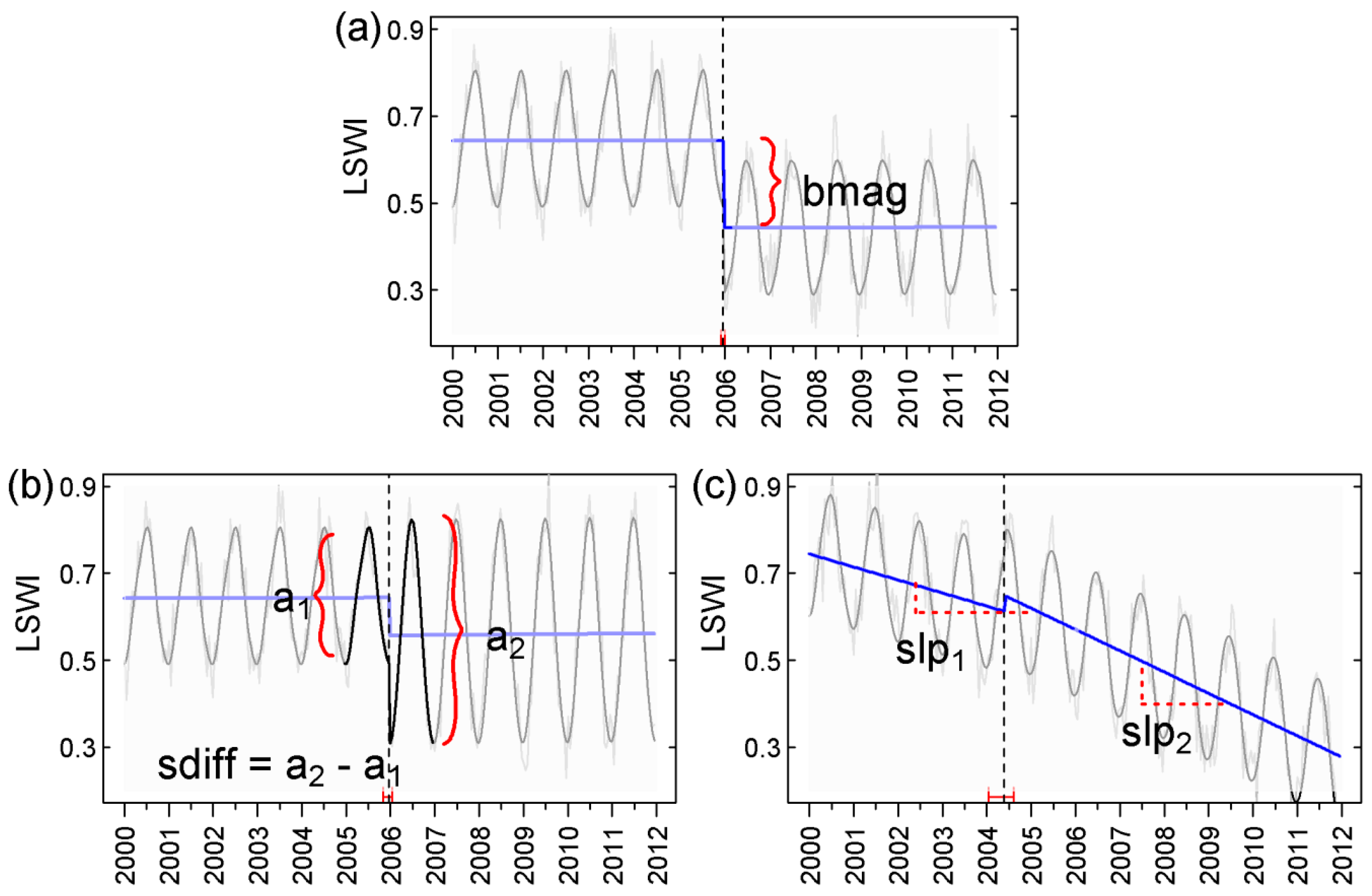
Forest clearing can be detected using the break magnitude, trend segment slope and/or changes in the seasonal component. Can combining these three components in a single change model improve detection accuracies compared to using only a single component?
(2)
It is reasonable to assume that specialized models outperform more general models, but it is not clear to what degree this is true with respect to forest types. Since a forest-type specific approach would require additional inputs, a generalised approach may be preferable for large-area mapping if accurate enough. Is it beneficial to map forest changes separately by forest type or is a single generalised change model sufficiently accurate?
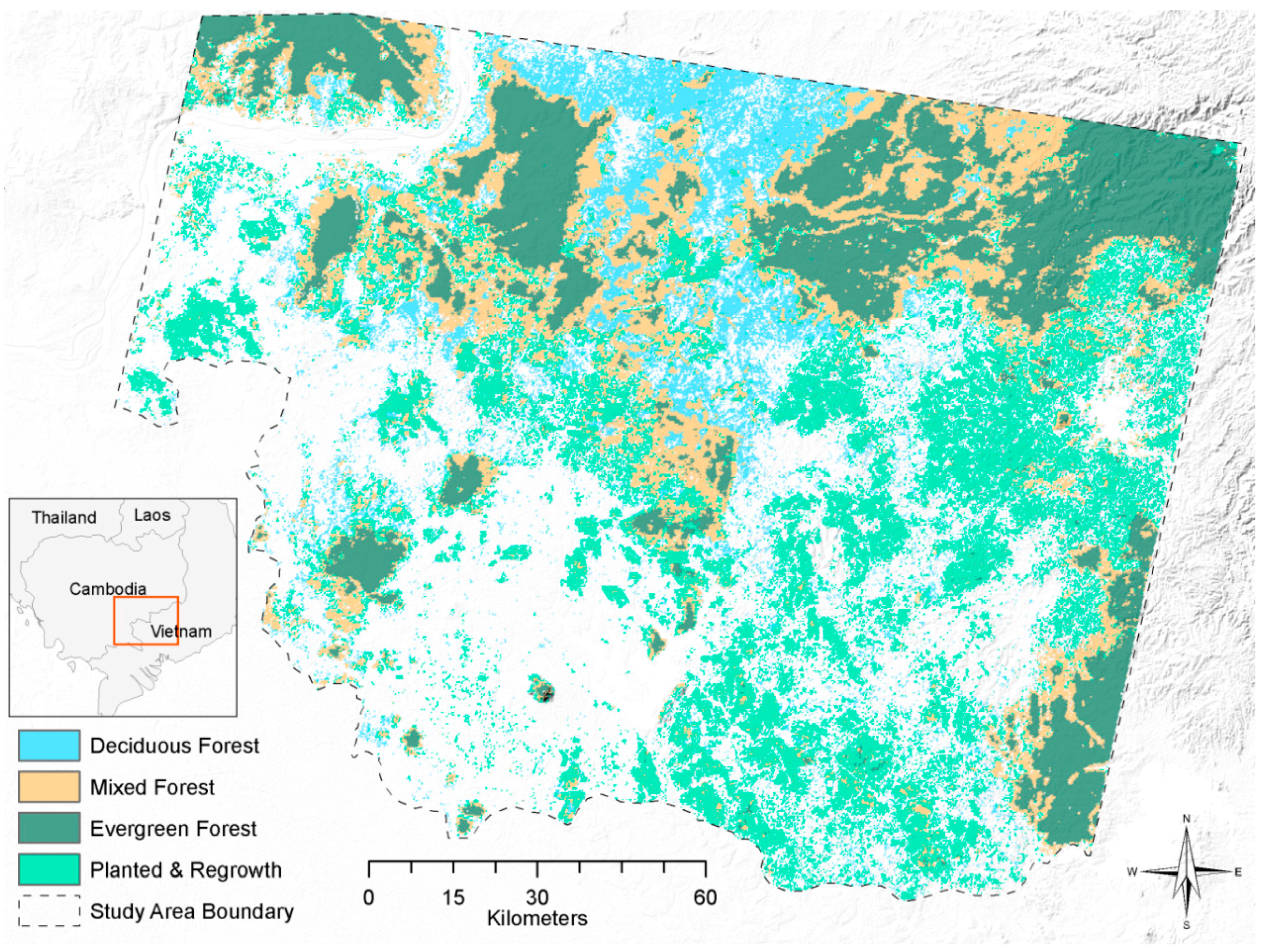
2. Study Area

The study area is located on the Cambodian-Vietnamese border and includes a number of typical forest types found throughout the larger region, including evergreen (29%), mixed-deciduous (22%), and dry-deciduous (15%) forest (Figure 1). Additionally, a significant proportion of tree cover is composed of plantation forest and forest regrowth (34%). Previous analysis has shown the area experienced significant forest loss from 2000–2012, mainly in the form of large-scale frontier forest clearing [45]. Seasons are divided into three distinct periods including a hot/dry season (March–May), a rainy season (May–October), and a cool/dry season (March–November). The study region is relatively flat with peaks of up to 900 m found mainly to the northeast.

3. Materials and Methods

We used Breaks For Additive Season and Trend (BFAST) [13,21] to extract breakpoint magnitude, trend, and seasonal components from filtered MODIS time series. We then used these as explanatory variables to predict per-pixel cleared forest probabilities using a non-parametric statistical model—Multivariate Adaptive Regression Splines (MARS). To assess the influence of forest type on change detection, we built separate change models for each forest type and then we compared the results with a generalised forest change model that ignored forest type.

3.1. MODIS Data and Processing

The 250-m MODIS 16-day Vegetation Indices (MOD13Q1) time series (February 2000–December 2012) was downloaded for tile ID h28v07 from the USGS server using the MODIS Reverb tool (http://reverb.echo.nasa.gov/reverb). Additional to the well-known Normalised Difference Vegetation Index (NDVI) [46] and Enhanced Vegetation Index (EVI) [47], we calculated the Land Surface Water Index (LSWI). A number of studies have used LSWI time series for land cover mapping [48,49]. The LSWI is sensitive to equivalent water thickness (g H2O/m2) and is therefore useful for detecting canopy water content or water stress, in contrast to canopy greenness. We used the NIR and resampled SWIR band provided by the MOD13Q1 product to calculate the LSWI:
NIR b 2    SWIR b 7 NIR b 2   +  SWIR b 7
These three indices provided the basis for MODIS time series analysis. We smoothed the time series using a weighted Savitsky–Golay filter and introduced seasonally adjusted window sizes for improved fitting during dry and wet seasons. For a detailed description of the MODIS processing and the filtering procedure, see Appendix A.

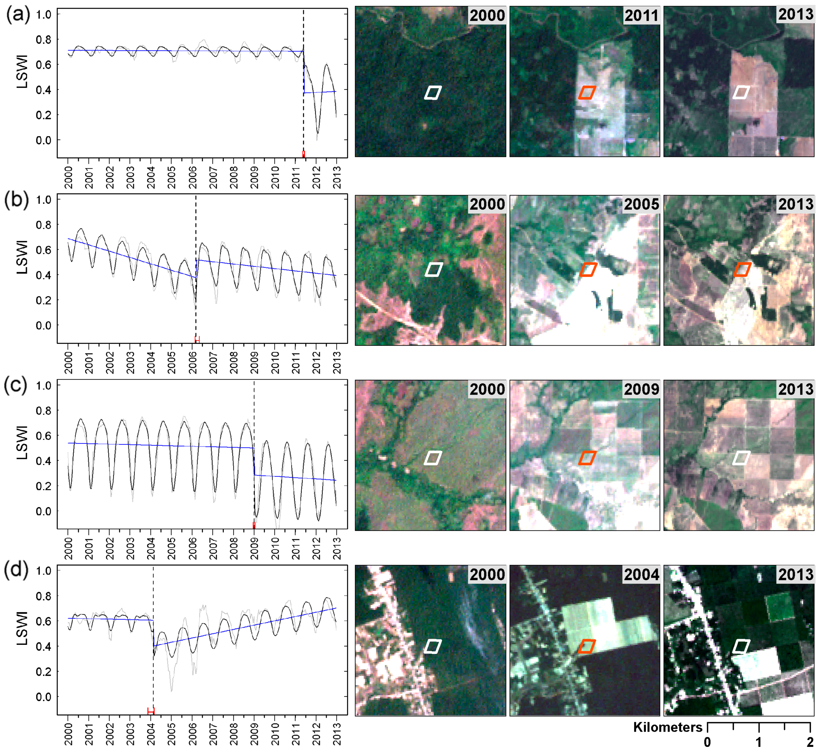
3.2. Extracting Breakpoints and Time Series Components Using BFAST

Time series analysis was performed on the filtered MODIS data using BFAST [13,21]. BFAST is an algorithm that combines structural break detection in time series with methods for decomposing the signal into seasonal, trend and remainder components. Piecewise linear trend and seasonal models are fitted to the time series using an additive decomposition model in the general form of:
Y t = T t   +   S t +   e t   ,    t = 1 , , n
where Yt is the observed data at time t, Tt is the trend component, St is the seasonal component, and et is the remainder component. The remainder component is the remaining variation in the data beyond what is explained by the seasonal and trend components. Before seasonal and trend models are fitted to the data, BFAST performs a test for abrupt changes in the time series. A number of different tests are available to detect structural breaks, including the Ordinary Least Squares (OLS) residuals-based Cumulative Sum (CUSUM) or Moving Sum (MOSUM) tests. If the test indicates a statistically significant change, breakpoints are estimated using the method of Bai and Perron [50], whereby the Bayesian Information Criterion is minimised to determine the optical number of breaks and break positions. We used a specific version of BFAST described by De Jong et al. [24], which is optimized to detect the most influential trend break in the time series. BFAST produces fitted seasonal and trend models based on the input time series (Figure 2). If there is an abrupt change in the time series it is indicated by a breakpoint. Optimal seasonal and trend models are then fitted for both time series segments on either side of the breakpoint. We used the ordinary least squares-moving sums (OLS-MOSUM) test with a significance level of 0.05 for detecting structural change within the MODIS time series. The MOSUM test for break detection is based upon the moving sums of OLS residuals within a user defined temporal window, or bandwidth. Similar to De Jong et al. [24], we choose the bandwidth of 40 observations. Since the number of 16-day time steps per year is 23, this gave a temporal window of just less than two years (i.e., 40/23).
We extracted three variables from the BFAST output that were potential predictors of forest clearing (Figure 2): the magnitude of the trend break (bmag), the seasonal amplitude difference between before and after a break (sdiff), and the most negative slope between each of the two trend segments (slp) (e.g., this would be the slope of second segment in Figure 2c). These three time series components were used as predictor variables for forest clearance modelling. The timing of clearances was estimated using the detected breakpoint.
BFAST is an open-source coding project available as an R package. For further details on its use and practical application see http://bfast.R-Forge.R-project.org/.

3.3. Classification for Comparing General and Forest-Type Specific Models

To address the question of whether forest-type specific change models improve the detection accuracy over a general change model, we classified the forest area into four classes for year 2000/2001: evergreen forest, mixed-deciduous forest, dry-deciduous forest, and a combined planted forest and forest regrowth class (see Appendix B for further details). We defined the forest area based upon the 30 m Vegetation Continuous Field (VCF) product for year 2000 [51] using a threshold of >15% tree cover [52]. All MODIS pixels with forest area above 75% were chosen for further analysis. For classification, we chose a random sample of 150 pixels per class and labelled them manually using a combination of Landsat and high resolution imagery from Google Earth. We used random forest [53] to classify each MODIS pixel using the above sample as training data and the three filtered time series (NDVI, EVI and LSWI) from February 2000–February 2001 as input data.

3.4. Change Model Training and Validation Data

For model training and validation we used a Landsat-based forest clearing map covering our study region created by Grogan et al. [45]. The map was produced by segmentation of Landsat time series using LandTrendr [12], and identifies stable forest and year of annual forest clearings in the period 2000–2012 with an overall accuracy of 86%. The forest area of the reference map was identical to that described in the previous classification step (Section 3.3). The reference map was aggregated from the original 30-m to the 250-m spatial resolution of the MODIS pixels. For this, we first projected the Landsat map to the MODIS sinusoidal projection. For each MODIS pixel we then calculated the cleared forest area proportion (Cp) for each year. The reference pixels with Cp values ≤0.05 were used as reference for stable forest, and pixels with Cp values >0.05 as reference for cleared forest.
Fully cleared MODIS pixels (Cp = 1) were more easily detected than partially cleared pixels (Cp < 1). To make the model results comparable between forest types, it was important that the training and validation sample for each forest type contained equal proportions of samples with similar Cp values. We selected a stratified random sample of 2000 pixels within each of the four forest types: 1000 forest clearance pixels and 1000 stable forest pixels. For the cleared forest sample we had five strata based on Cp value intervals: 0.05–0.24 (n = 130), 0.25–0.49 (n = 170), 0.50–0.75 (n = 200), 0.75–0.99 (n = 270) and 1 (n = 230). The sample size (n) for each clearance strata was proportional to the Cp frequency distribution using the same strata intervals for all forest clearance pixels (i.e., without distinguishing between forest type). We split the cleared and stable forest sample in half for each forest type, 50% for model training and 50% for model validation.
To ensure a minimal error in the training and validation samples, we manually screened all samples using time series of Landsat image chips (similar to Cohen et al. [54]), temporal-spectral profiles, and additional imagery from Google Earth where available. We removed and replaced any change or stable samples that were incorrectly labelled.

3.5. Modelling Forest Clearance Using Time Series Components

To discriminate between changed and stable forest pixels we modelled our binary response (cleared or stable) as a function of three predictor variables, bmag, sdiff, and slp. The relationships between the predictor variables and the binary response varied among forest type and were often non-linear. For example, clearance events were associated with both positive and negative sdiff values. A regression method capable of handling more complex interactions was therefore required. In this study we used Multivariate Adaptive Regression Splines (MARS). MARS is a non-parametric adaptive regression technique in which non-linear relationships between response and predictor variables are described via a series of piecewise spline basis functions [55,56]. Each segment of the fitted function is separated by a “knot” in a model that initially over-fits the training data. The final model is then simplified using a step-wise cross-validation procedure which incorporates a penalty term dependent on model complexity. The MARS model assumed a binomial error distribution, which ensured the values of the response variable were constrained between 0 and 1. For our models, predicted probabilities closer to 1 indicated higher likelihood of being cleared, while values closer to 0 were more likely to be stable forest.

3.5.1. Analysis of the Relative Importance of Time Series Components Clearance Predictions

To understand how well each individual variable predicts forest clearance, we first built separate forest-type specific change models using single variables only. We proceeded to combine predictor variables to test whether this improved the predictive power of the model and to assess which variable combination provided the most accurate results. We evaluated the performance of each model using receiver operating characteristic (ROC) curves. ROC curves illustrate the performance of binary response models by plotting the model sensitivity (true positive rate) against specificity (true negative rate) as the predicted probability threshold is varied. The area under the ROC curve (AUC) is a measure of the models predictive performance, with values of 0.5 indicating no discriminatory ability, and values of 1 indicating perfect discrimination. We made ROC curves using the validation data to assess model performance.

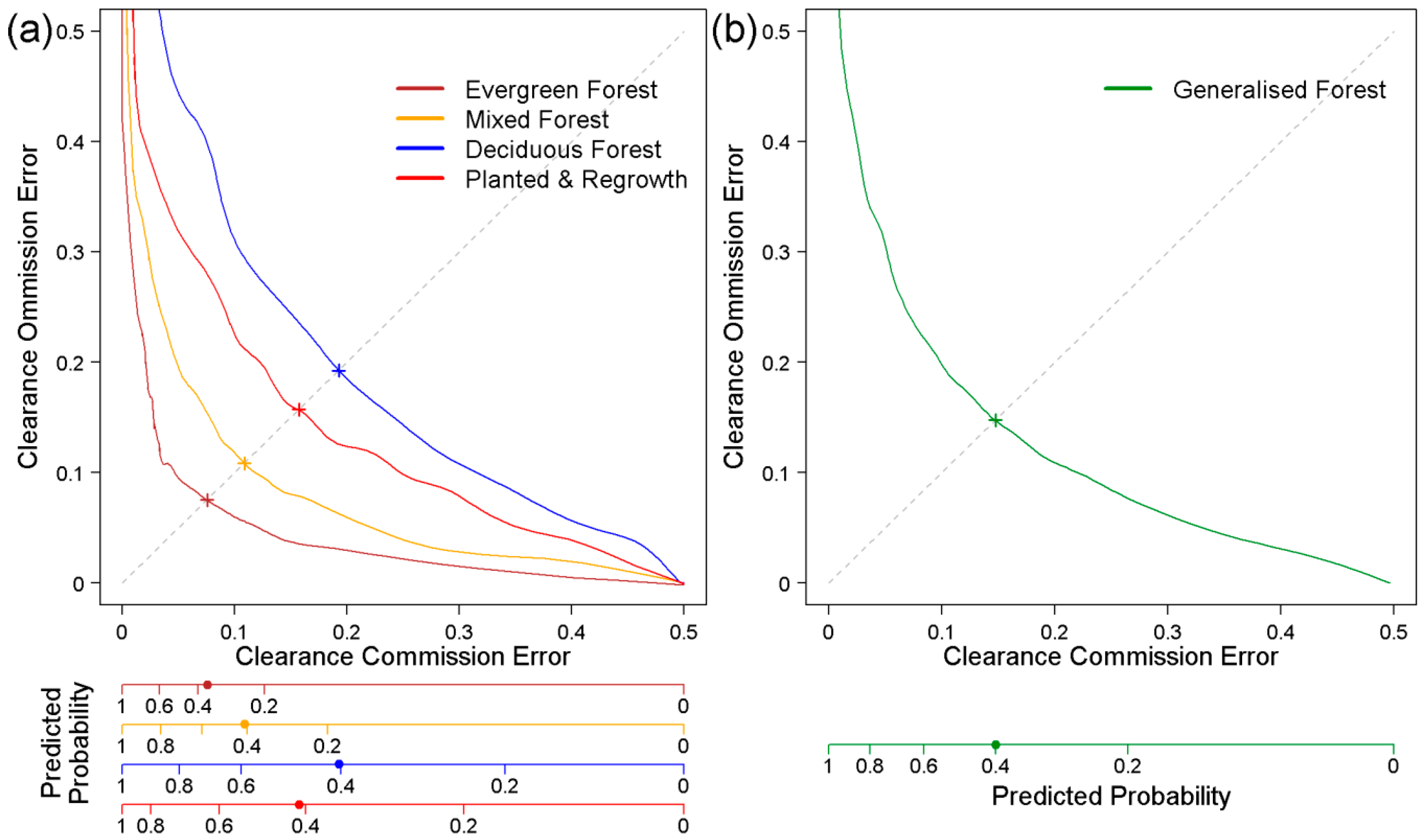
3.5.2. Comparison of Forest-Type Specific and Generalised Models

To determine the effect of forest type on clearance detection accuracies, we combined all training data to train a generalised forest change model using the same predictor variable combinations. Using the validation sample we then analysed the distribution of commission and omission errors among each forest type. Because our model (MARS) predicts class probabilities, it was necessary to translate the probabilities into discrete class memberships, but rather than selecting a single threshold value of probability (e.g., one that maximizes the overall accuracy), we estimated commission and omission errors for the entire range of probability thresholds (i.e., from 0–1). The resulting error curves were then plotted to examine differences between the forest-type specific and general approaches and to identify suitable probability thresholds. Although, the definition of a suitable threshold is user-specific, we selected thresholds that lead to balanced commission and omission errors.

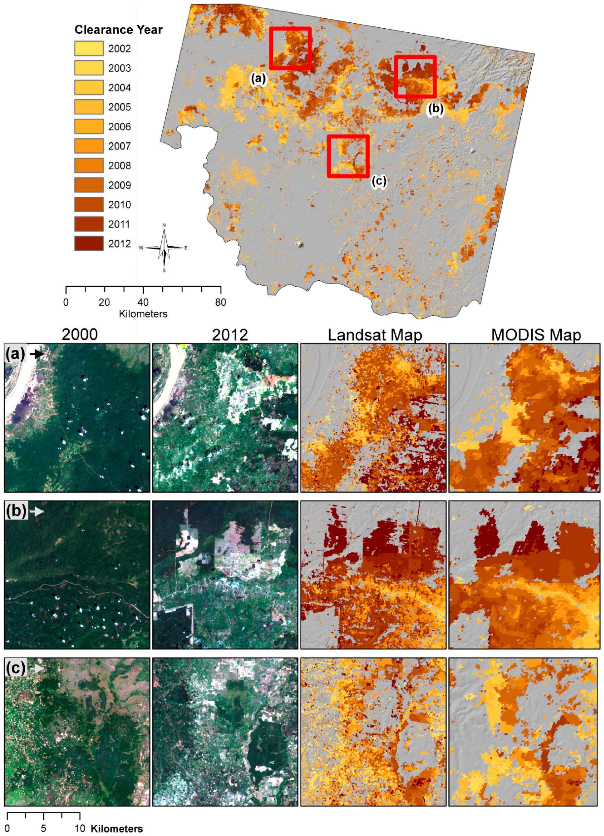
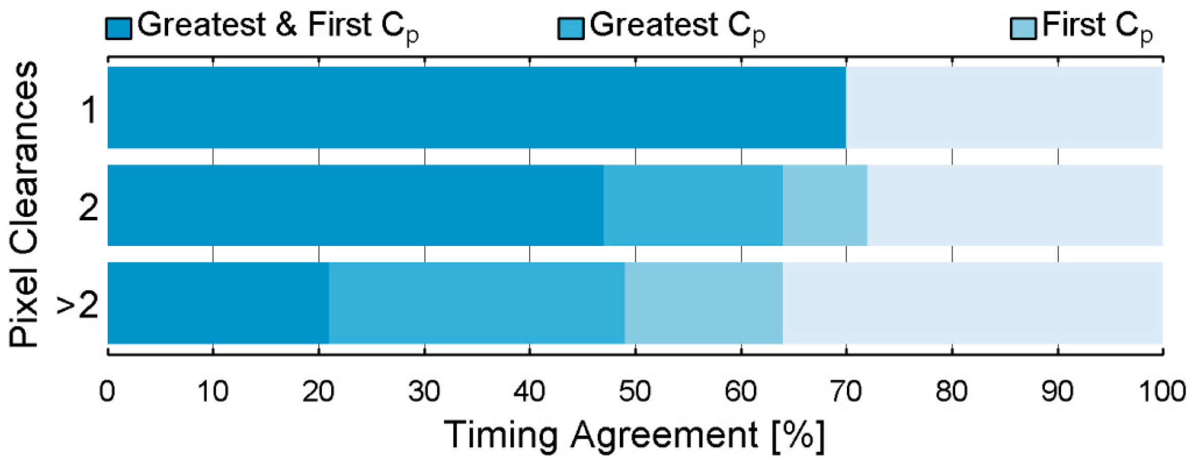
3.6. SPATIAL/Temporal Accuracy and the Effects of Sub-Pixel Clearances

We used the validation sample to explore the effects of sub-pixel clearances on spatial accuracy (detection of clearing location) and timing of forest clearance. To analyse the effects of sub-pixel forest clearings on locational detection accuracy we generated histograms of omission error for the cleared forest class using Cp intervals of 10%. The temporal accuracy of the MODIS forest clearing map can be defined in a number of different ways when considering the effects of low resolution bias. If a single clearance occurs within a pixel then the mapped year of clearance using BFAST should relate to the actual year of the forest clearing. If however, there are multiple clearing events spanning two or more years, assigning a year label is not unambiguous. We assessed the temporal accuracy of the MODIS forest clearing map using two methods: (1) the year of maximum cleared area; and (2) the first year of forest clearing. We considered the timing of the clearance correct if it matched the reference sample year ± 1.

4. Results

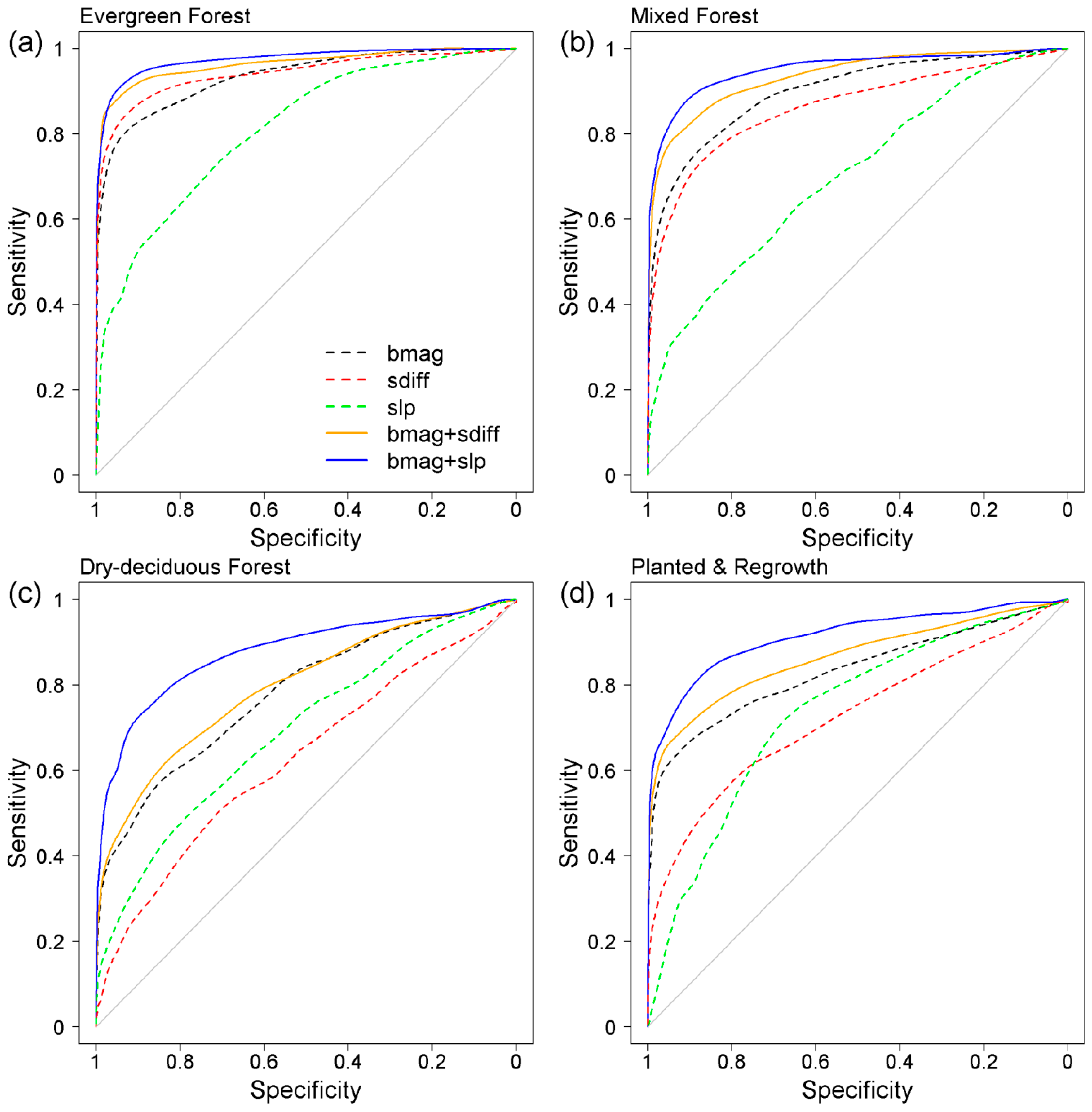
4.1. Time Series Components and Their Effect on Forest Clearing Detection Accuracy

All three time series component variables: break magnitude (bmag), seasonal amplitude difference (sdiff), and negative trend slope (slp), were found to be associated with forest clearances (Figure 3). High magnitudes breaks were the most common indicator of change (Figure 3c,d) and were often accompanied by a significant change in the seasonal amplitude (Figure 3a). Forest clearance was also associated with steep negative trends before or after the breakpoints (e.g., Figure 3b). Among the spectral indices tested, LSWI performed best overall when compared to NDVI and EVI. In the interest of brevity, we present results using the LSWI only. Model results (ROC curves and AUCs) using NDVI and EVI can be found in Appendix C.
Overall, bmag was the best performing single predictor of forest clearance (Figure 4). sdiff was a slightly better predictor of clearance than bmag in evergreen forest and gave comparable accuracies to bmag in mixed forest, but was much less effective in planted and regrowth forest and especially so in dry-deciduous forest. The slp variable was the least effective single indicator of change in evergreen and mixed forest, but performed slightly better than sdiff in dry-deciduous forest and forest regrowth.
Using multiple predictors improved the performance of the change models in each forest type. Combining bmag and sdiff as explanatory variables improved model results with AUC increases ranging from 0.01 in dry-deciduous forest to 0.04 in mixed forest when compared to using bmag alone (Table 1). Combining bmag and slp variables showed further increases in predictive power, with AUC increases ranging from 0.04 in evergreen forest to 0.11 in dry-deciduous forest when compared to using bmag alone. Using a combination of all three variables only slightly improved the model performance in evergreen forest compared to the bmag + slp model, with no further improvements gained in the other three forest types. Although the models performed very well in each forest type, there was notable variability. Higher AUCs were present in evergreen (0.98) and mixed (0.96) forest, and comparably lower values were found in planted and regrowth forest (0.92) and dry-deciduous forest (0.89).

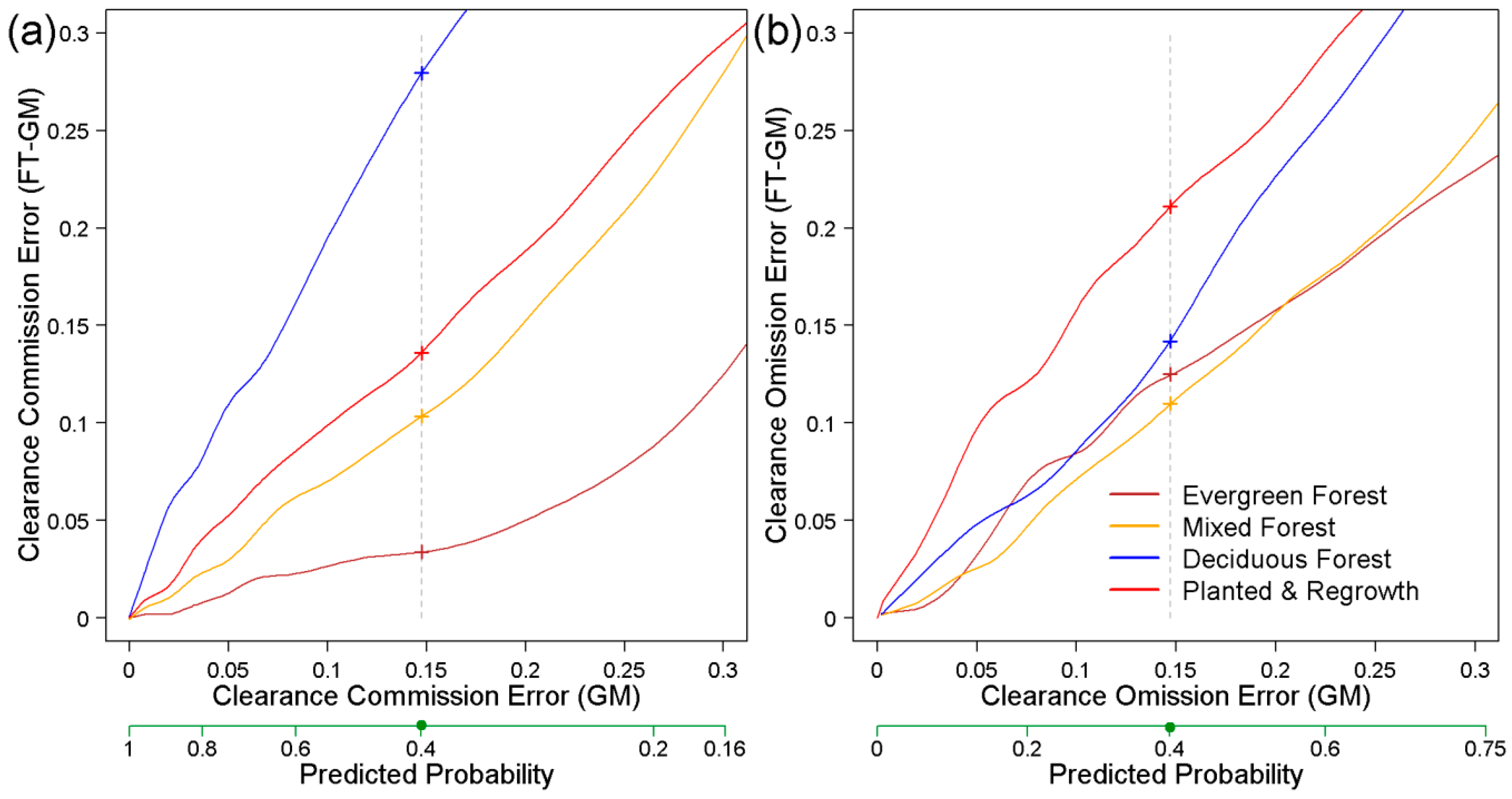
4.2. Generalised versus Forest-Type Specific Models

By plotting omission versus commission errors for each model, any point on each error curve corresponds to a specific model probability threshold (Figure 5). Using forest-type specific models, errors were lowest in evergreen forest, followed by mixed forest, planted and regrowth forest and then dry-deciduous forest (Figure 5a). The shapes of the curves highlight the differences in model error sensitivity. For example, for forest clearance commission errors ranging between 0.05 and 0.25 the range of omission error in the dry deciduous forest was largest at 0.42–0.18 showing high sensitivity. Conversely, the corresponding range of omission error for evergreen forest was lowest at 0.09–0.02, displaying much lower sensitivity. When probability thresholds were chosen that balanced commission and omission errors, evergreen forest showed the lowest error at 0.08, increasing slightly for mixed forest (0.11), followed by planted and regrowth forest (0.16) and dry-deciduous forest (0.19) (Figure 5a). The average error balance for all validation samples using forest-type specific models was 0.14.
When using the generalised forest model, there is only one error curve, which represents the overall omission versus commission error curve, i.e., all forest without respect to forest type (Figure 5b). When a probability threshold was selected that balanced commission and omission errors, the generalised forest model achieved almost the same overall error rate as the forest-type specific models (0.15). Figure 6, however, illustrates how commission and omission errors using the generalised model were distributed between the four forest classes across a range of probability thresholds, allowing a comparison to the forest-type specific models. When the overall balanced error from the generalised model of 0.15 was separated by forest type, the errors were notably unbalanced and varied considerably, summarised in Table 2. Evergreen and dry-deciduous forest types were the two most affected by error imbalances, ranging from 0.09 to 0.14, respectively. The regrowth class was slightly less affected by the imbalance, while the mixed forest class remained virtually unaffected.
When compared to forest-type specific models, the generalised model consistently favoured higher commission/lower omission error in dry-deciduous forest, balanced mainly by a lower commission/higher omission error in evergreen forest. Overall, mixed forest and planted and regrowth forest error rates were less impacted by the choice of model. Using data represented in Figure 5 and Figure 6, a further two example tables are provided in Appendix D showing that this result holds true across a range of possible user-defined thresholds.

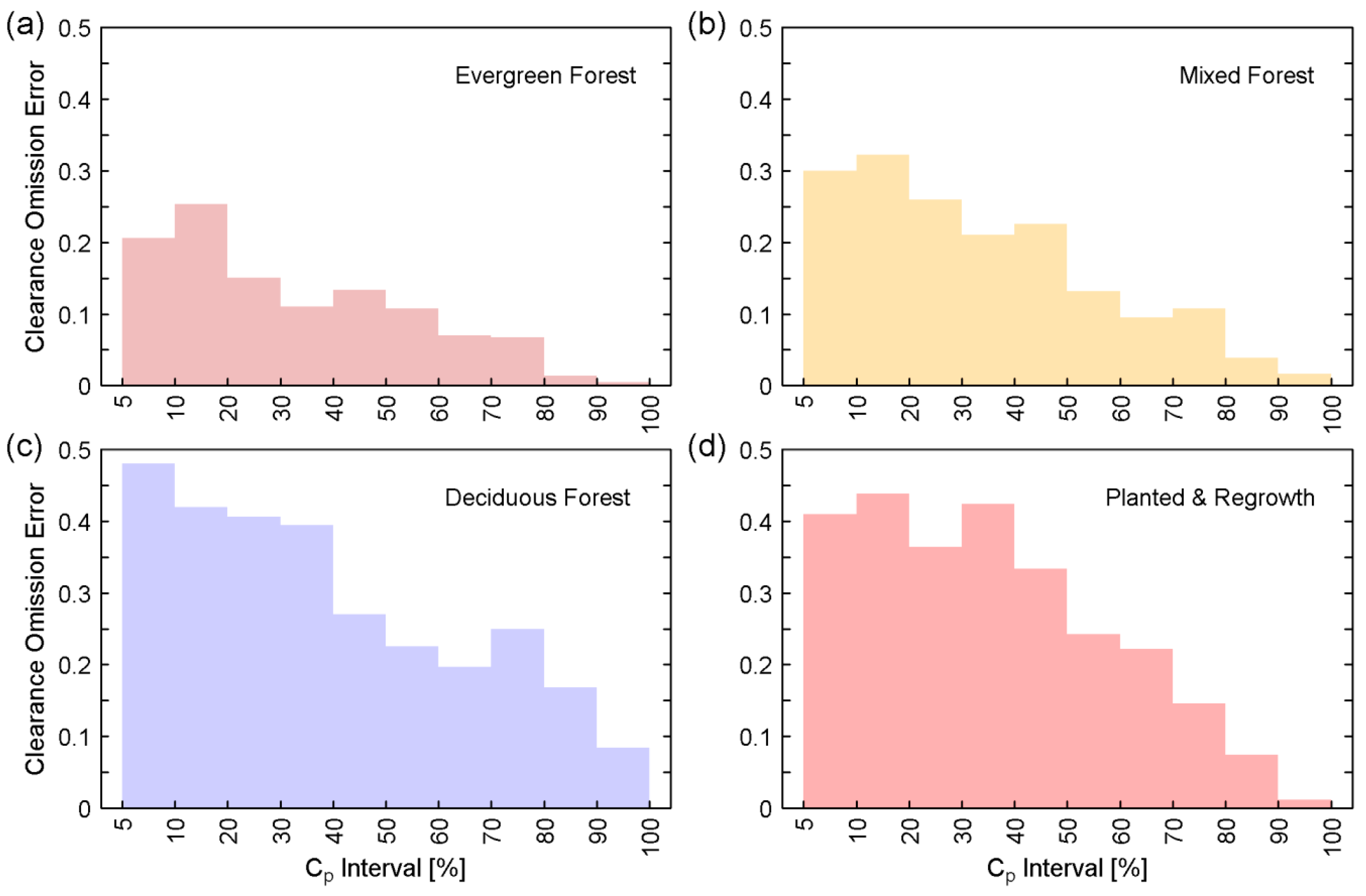
4.3. Forest clearance Mapping and Sub-Pixel Change

We mapped forest clearance using the forest-type specific model with bmag and slp as predictor variables and choosing a balanced commission and omission error. There was generally good agreement between the Landsat reference map and the 250-m MODIS map (Figure 7). The majority of change omission error was caused by clearances that occurred at the sub-pixel level and is therefore product of inherent low resolution bias (Figure 8). For clearance pixels that have Cp levels below 50%, the omission error was highest at between 0.17 (evergreen) and 0.40 (dry-deciduous). Omission error decreased linearly as Cp increased reaching a minimum ranging from 0.01 (evergreen) to 0.08 (dry-deciduous) for Cp values of 90%–100%.
Sub-pixel forest clearance also affected the timing assigned to clearance pixels since multiple clearances may occur at different times within the same MODIS pixel. When only one annual clearance occurred within a MODIS pixel the timing agreement using LSWI matched the validation data ±1 year for 70% of the samples (Figure 9). As the number of annual sub-pixel clearances increased, the timing labels assigned to cleared pixels were largely shared between the year with the greatest Cp value and the year of the first Cp occurrence. Agreements using these two matching criteria remained above 60% as the number of annual clearances increased.

5. Discussion

5.1. Combining Break Magnitude, Trend, and Seasonal Components

Combining trend and seasonal information with the break magnitude improved model performance, albeit to varying degrees, depending on forest type. A high break magnitude (bmag) was typical of the sudden deforestation events in the study area described by Grogan et al. [45], primarily large-scale rubber plantation expansion and smallholder clearances for agriculture. Linear trends have shown to be highly useful change indicators by many studies [12,15,19,20]. Overall, we found the addition of the negative trend variable (slp) enhanced model performance more than the addition of the seasonal amplitude difference (sdiff). Previous forest disturbance studies have modelled seasonality with the primary aim of removing the seasonal affects from the underlying trends [22,23]. Here we incorporated pre- and post-disturbance seasonal information into the change model and showed that it can also be a useful indicator of change, especially in low seasonality forest.

5.2. Model Sensitivity to Forest Type and Seasonality

Each model displayed consistently poorer performance moving from low to high seasonality forest (Table 2). This suggests an association between model accuracy and the gradient of forest seasonality, or degree of deciduousness, ranging from dry-deciduous to evergreen forest. Dry season leaf senescence can cause confusion in forest change analysis which can lead to higher error frequently reported in deciduous classes [57,58,59]. Besides seasonal variation in reflectance increasing with forest deciduousness [60], there can also be considerable natural inter-annual variation linked to changing climate and variable rainfall patterns [61,62,63]. This presents a major challenge for methods that use ridged seasonal models as they often model a constant average seasonality, failing to capture the natural variation. In tropical-dry forests characterized by high inter-annual seasonal variability, it does not seem ideal to use a seasonal model that assumes regular or stable seasonality—as does BFAST and other seasonal model approaches (see Zhu et al. [23] and Zhu and Woodcock [14]). Zhu and Woodcock [14] mapped land cover change with high accuracies in a humid continental climate using an approach that assumed phenology was consistent over time for stable land covers, but noted this could be problematic for drier regions. To address these shortcomings Jamali et al. [64] used a seasonal-trend decomposition procedure which allowed the seasonal model to vary from season to season. However, although this approach may better account for inter-annual forest variability, it remains uncertain if the variation captured in the seasonal model is due to natural variation or human induced change. This uncertainty has the potential to mask real disturbances from being evident in the trend component. A promising alternative might be to account for seasonal variation in the model by using external regressors. Dutrieux et al. [65] take such an approach in a recent Landsat-based change detection study in tropical dry forests by adjusting the seasonal NDVI model using MODIS based measures of inter-annual variability, with encouraging results. They also tested a measure of rainfall variability as an external regressor but with poorer results. Despite this, the use of climatic variables (e.g., soil moisture) to account for inter-annual variability in optical time series remains to be fully explored and further investigation may yield more favourable outcomes.

5.3. Model Sensitivity to Spectral Indices

We found that change models using LSWI time series performed better overall compared to the more commonly used NDVI and EVI. The LSWI is based on the spectral differences found between the NIR and SWIR bands. SWIR bands and associated indices are sensitive to canopy moisture and forest structure [66], and have been shown to be more responsive to a variety of disturbance types compared to indices based on NIR and VIS bands which target canopy greenness [12,45,67,68]. A possible explanation for this is that tropical vegetation greenness can recover rapidly soon after forest clearing as the herb layer and young saplings grow vigorously due to increased light levels, leading to an overall reduction in sensitivity when using greenness as a disturbance indicator. Hais et al. [68] demonstrated this affect in forests of Central Europe and found SWIR based indices to be more sensitive to forest disturbances. Another major advantage of SWIR based indices (and SWIR emphasizing transformations such as tasselled cap wetness) are their relative robustness to atmospheric water vapour and aerosols [69]. This property can further enhance the signal-to-noise ratio [70], leading to better characterisation of forest conditions and ultimately contributing to higher mapping accuracies.

5.4. Generalised versus Forest-Type Specific Models

Although overall accuracies were similar using forest-type specific models and a generalised forest model, applying separate models allowed more control over the error distribution among the different forest types. Compared to forest-type specific models, the generalised model consistently mapped forest clearance in dry-deciduous forest favouring lower omission error, but higher commission error. This was balanced by favouring lower commission/higher omission error in mainly evergreen forest. Our results suggest that accounting for forest type can improve forest clearance mapping in areas characterised by diverse forest types such as Southeast Asia. It seems particularly important to separate dry-deciduous and evergreen, seen as they have the largest swing of error imbalances using the generalised approach (Table 2). We gave equal weight to each forest type in our analysis. When considering discriminating forest type for forest clearance mapping thought should be given to the proportion of different forest types in the study region to evaluate the trade-offs in potential improved error distribution versus applying an extra classification step. This is likely more important for large area mapping where forest type can vary considerably. Discrimination of forest type can be made using a base map, as used in this study, or done on-the-fly during the time series analysis using the spectral information.

5.5. Forest Disturbance Mapping Using BFAST

Previous forest disturbance based studies using BFAST have mapped on the Landsat scale using breakpoints alone (i.e., no magnitude thresholding) to detect change [65,71]. However, DeVries et al. [22] showed that thresholding the break magnitude can be an important step distinguishing change from stable forest. Here we demonstrate how multiple BFAST components, combined with thresholding, can be used for effective forest monitoring using in MODIS time series. We used the single most influential break to identify forest clearance. Using multiple breakpoints may offer a more detailed summary of the pixel history—e.g., ability to capture multiple disturbances and trajectories. We also confined our study to monitor forest clearing, but the approach could also be adapted to include forest recovery, similar to DeVries et al. [72]. Although BFAST can handle unfiltered data, we found in the preliminary testing phase of our analysis that applying a smoothing filter improved forest clearance detections. MODIS 16-day time series products can be exceptionally noisy in the tropics, in part due to errors related to deficiencies in aerosol and cloud screening [73,74,75]. Time series composites generated using more advanced cloud screening and atmospheric correction techniques have shown to dramatically reduced time series noise [75] and may eliminate the need for data filtering.
Another shortcoming of BFAST and other similar time series models is that by using linear segments to describe underlying trends, they assume vegetation trends are linear processes. It has been known for some time that land cover change can often occur along non-linear multidirectional pathways [76]. Both abrupt and slowly occurring disturbances in land cover such as forest clear-cutting, fires, insect outbreaks and logging can result in non-linear changes to vegetation cover [77]. Similarly, natural climatic processes such as short- or long-term changes in rainfall patterns or temperature may induce a non-linear response form vegetation cover. Jamali et al. [78] tried to account for such non-linear processes by describing long term trends using polynomials and found it to adequately describe general non-linear change trajectories in the Sahel. The future challenge will be to incorporate non-linear change processes into change detection time series models.

5.6. Relevance for Forest Monitoring Systems

Robust forest monitoring systems are becoming increasingly more important, especially for conservation efforts and global climate initiatives such as REDD+. Tropical environments such as Southeast Asia present a unique challenge for retrospective and on-going forest monitoring, primarily due to data availability. For example Broich et al. [39] have shown cloud free Landsat observations for Indonesia are between 0 and 5 per year. Such data scarcity limits the capabilities of Landsat time series in these regions. Further monitoring limitations arise from technical capacities and budget constraints. For these reasons many advocate the combined use of sensors [79], drawing from the advantages of each in an integrated monitoring system. Such data-fusion approaches have been developed, e.g., by Hansen et al. [33], who integrated Landsat and MODIS to estimate forest clearing area in the humid tropics; or Potapov et al. [80], who used a similar approach in North America. Our results demonstrate how MODIS can be used to provide valuable information on location and timing of forest clearance events with high accuracy in a tropical dry environment. Our study region was relatively small however, so it is necessary to test if the approach can be successfully applied to a national or regional scale. Such forest clearance maps at the 250-m scale can be used to provide fast, up-to-date information on deforestation hotspots, where mapping efforts can be concentrated, or used as a stratification tool for estimating forest change area using probability based sampling [33,81,82]. It should be noted, however, that low resolution bias can limit the capacity of the MODIS sensor in regions with clearances occurring at smaller scales (e.g., mosaic forest clearing, or shifting cultivation). Dense intra-annual time series at medium resolution (20–30 m) will soon be available for the tropics pending the fusion of Landsat and Sentinel imagery, which will improve the ability to capture these smaller scale clearances at high temporal resolutions. Given the spectral similarities between MODIS and Landsat/Sentinel sensors the methods described in this manuscript should be readily transferable to future medium resolution applications.

6. Conclusions

Methods for forest monitoring using dense time series are advancing rapidly. This study demonstrates how combining break magnitude, trend, and seasonal components can improve forest clearance mapping when compared to using just the break magnitude alone. Our study indicates that forest type has significant influence on model performance, with lower accuracies in dry-deciduous forest and higher accuracies in evergreen forest, with mixed forest and forest regrowth accuracies lying in between. This suggests a relationship between the model performance and the gradient of seasonality. We also demonstrate that modelling forest clearance with respect to forest type, as opposed to using a generalised forest model, offers a more flexible approach and can ensure that the error levels within each forest type are optimally distributed by the user by choosing forest-type specific thresholds. The division of forest type is therefore important for regions such as Southeast Asia where diverse forest types with different phenology and spectral response to forest clearing can be found. It is especially relevant for large area mapping as there is a higher likelihood different forest types will be included in the analysis. From a forest monitoring perspective, the accuracies achieved using our approach show promising potential; however, it remains to be tested if the models can be applied over larger regions, while maintaining similar performance levels. Our methodological approach shows the potential usefulness of MODIS for rapid assessment of timing and location of forest cover change over large areas which can form part of an integrated monitoring system. These methods can also be useful for future medium resolution applications based on Landsat and Sentinel datasets.

Acknowledgements

This research is part of the research project entitled, Impacts of Reducing Emissions from Deforestation and Forest Degradation and Enhancing Carbon Stocks (I-REDD+). I-REDD+ is funded by the European Community’s Seventh Framework Research Programme (Call number: FP7-ENV-2010, Grant number: 265286). More information can be found at: www.iredd.dk.

Author Contributions

The paper was conceived and designed by Kenneth Grogan with assistance from Dirk Pflugmacher, Rasmus Fensholt and Patrick Hostert. Kenneth Grogan analysed the imagery with technical support from Dirk Pflugmacher and Jan Verbesselt. The manuscript was written by Kenneth Grogan with input from all co-authors.

Conflicts of Interest

The authors declare no conflict of interest.

Abbreviations

The following abbreviations are used in this manuscript:
AUCArea under (ROC) curve
BFASTBreaks For Additive Season and Trend
bmagThe magnitude of the trend break
CECommission error
CpCleared proportion of MODIS pixels
EVIEnhanced vegetation index
FT-GMForest types within the generalised forest model
GMGeneralised forest model
LSWILand surface water index
MARSMultivariate adaptive regression splines
MODISModerate Resolution Imaging Spectroradiometer
NDVINormalised difference vegetation index
NIRNear-infrared
OEOmission error
OLS-MOSUMOrdinary least squares-moving sums
PProbability
REDD+Reduced emission from deforestation and forest degradation
ROCReceiver operating characteristic curves
sdiffThe seasonal amplitude difference between before and after a break
slpThe most negative slope between each of the two trend segments
SWIRShortwave-infrared
USGSUnited States Geological Survey
VCFVegetation continuous field

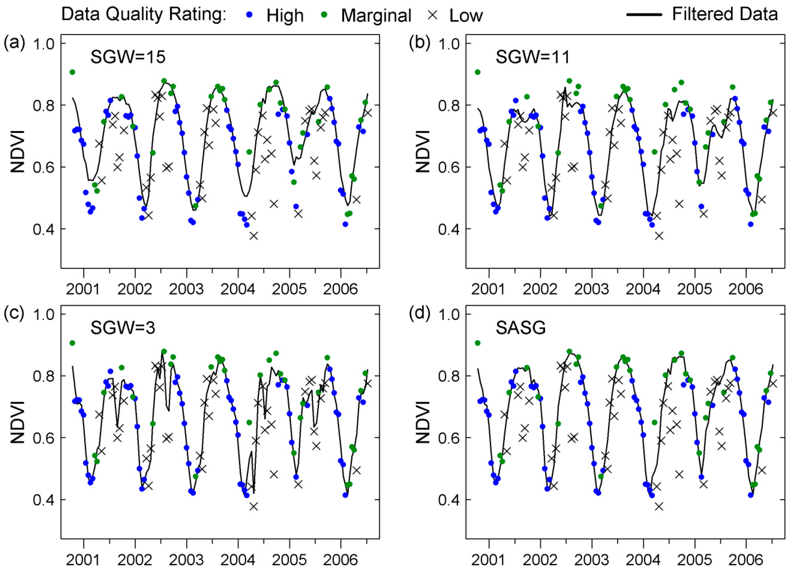
Appendix A. MODIS Data Processing and Filtering Procedure

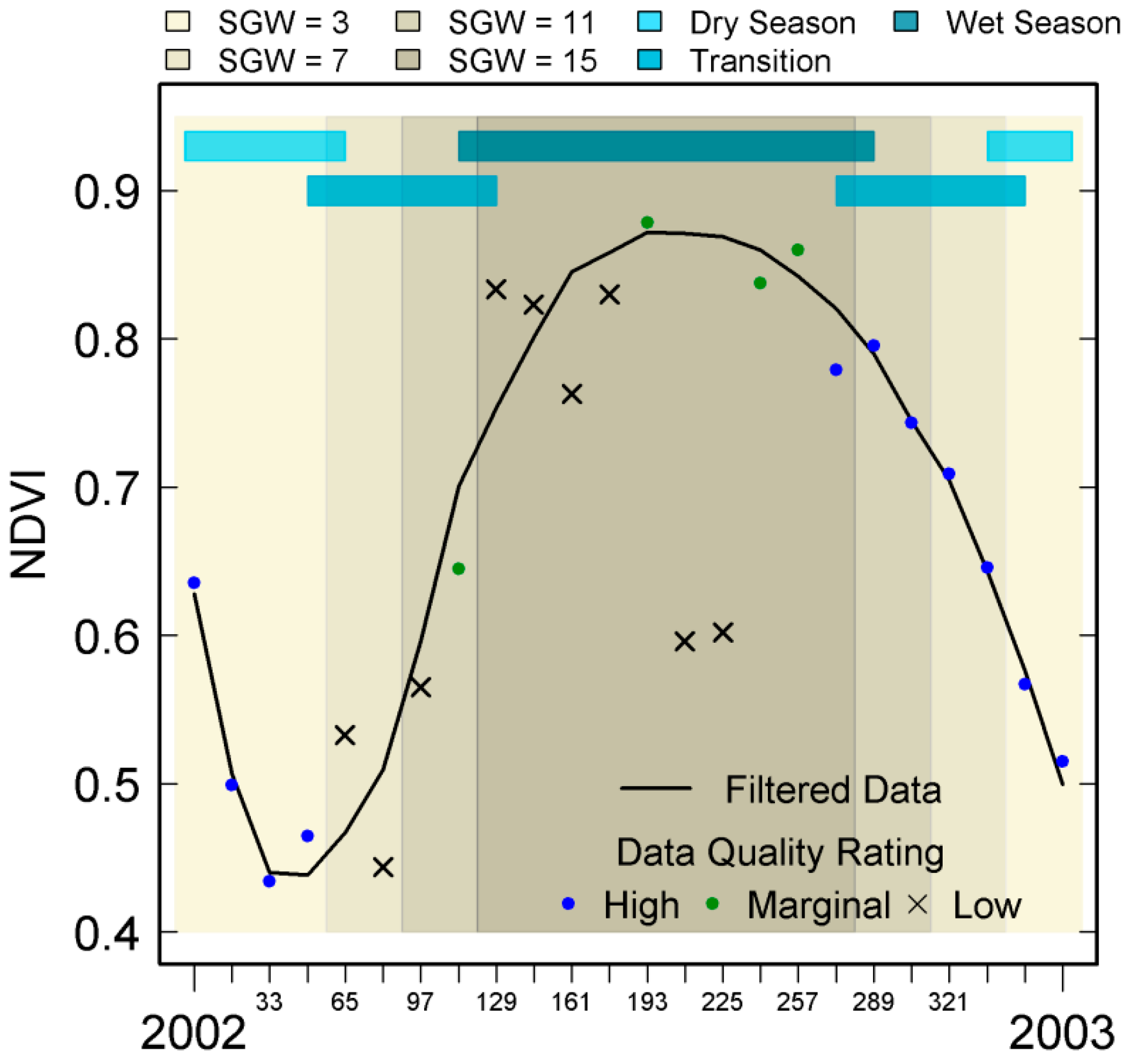
A1. MODIS Data Quality Rating

To filter MODIS time series observations we distinguished three levels of data quality based on pixel-wise MODIS quality flags: high quality, marginal quality, and low quality. High quality data were defined as cloud-free observations with low or medium aerosols, and low view (<40 degrees) and sun (<60 degrees) angles. Marginal quality data were defined as cloud-free observations with possible high aerosols and/or high view and sun angles. All remaining cloudy data were rated as low quality. Two additional modifications based on blue band reflectance were made to accommodate known quality flag issues regarding cloud and high aerosol screening [73,74,83,84]. First, all observations with a blue reflectance of >0.11 were considered contaminated by cloud or very high aerosols and therefore given a low quality rating. Second, pixels that were labelled as cloudy by the MODIS quality flags but had very low blue band reflectance (<0.025) were labelled as marginal quality. These steps lowered the quality ratings of some observations with potential severe atmospheric contamination, while increasing the rating of likely clear sky observations.

A2. MODIS Data Filtering and Assembly

To reduce noise in each time series we applied a weighted iterative Savitsky–Golay filter. While testing different filter parameters, we found that varying the filter width with the season improved the results. During the wet season, data quality is generally low due to the influence of cloud cover. A wide window size was therefore better suited to this period. However, a wide filter window did not produce a good fit during the dry season, where it often failed to effectively capture the more rapid changes associated with leaf flushing and senescence. Because dry season data are of much higher quality compared to the wet season, a narrower filter can be used here to capture these important phenological features. We therefore applied the Savitsky–Golay filter using varying window sizes that we tailored to the seasonal patterns of the study region. In the following we referred to this approach as Seasonally Adjusted Savitsky–Golay filter (Figure A1). As the seasons transition from dry to wet, the Savitsky–Golay window size was gradually increased (3 > 7 > 11 > 15). The window size was then gradually reduced when the seasons changed from wet to dry (15 > 11 > 7 3). We used a combination of Timesat [85] and a script developed in R to produce the final filtered time series. A median filter using 1.5 standard deviations was first applied to the time series to remove any extreme data spikes. The weighting used for the Savitsky–Golay filter was based upon the data quality rating in the previous step. A weight of 1 was assigned to high quality data, 0.8 to marginal quality data, and 0.5 to low quality data. We found that the seasonally adjusted filter retains the benefits of both wide and narrow window sizes though the annual seasonal cycle, estimating an improved fit when data quality is generally low, while preserving data values when quality is high (Figure A2).
We replicated the final year of MODIS data (year 2012) and appended it to the end of the time series as this improved the detection of forest clearances that occurred in the final year when using BFAST.
Figure A1. Description of the Seasonally Adjusted Savitsky–Golay filter. Seasons and season transitions are indicated by the horizontal blue bars. Savitsky–Golay window size (SGW) ranges from three observations during the dry season to 15 observations during the wet season.
Remotesensing 08 00657 g010
Figure A2. Example of filtered data in dry deciduous forest. Standard Savitsky–Golay filter with window sizes of 15 (a); 11 (b); and three (c); and the Seasonally Adjusted Savitky–Golay (SASG) filter (d). Wider window sizes are better suited to poor quality data during the wet season, while narrow windows are better suited to higher quality data available during the dry season. The SASG preserves the advantages of both. SGW = Savitsky–Golay window size.
Remotesensing 08 00657 g011

Appendix B. Distinguishing Forest Class

We divided the forest area into four classes: evergreen forest, mixed-deciduous forest, dry-deciduous forest, and a combined planted forest and regrowth class. Separation of the classes was similar to that described by Grogan et al. [45]. Dry season false colour composites using a combination of visible, near-infrared, and shortwave-infrared bands provided optimal separation between different classes. Evergreen, mixed-deciduous and dry-deciduous forest could be separated using early dry season imagery (Figure B1a). Evergreen forest displayed little phenological variance throughout the dry season, and was characterized by almost complete canopy cover. Dry-deciduous forest experienced very large phenological variation throughout the year due to leaf senescence.
To distinguish rubber from other forest/woody vegetation, imagery from the late dry season/early wet season was best. At this time of year rubber is in the foliation phase and has a distinct reflectance in the near-infrared and shortwave-infrared bands [86]. Using false colour composites (TM/ETM RGB = bands 4, 5, and 2, OLI RGB = bands 5, 6, and 3) rubber appeared a distinctive orange colour (Figure B1b) and was readily distinguished from evergreen forest (bright red, Figure B1b-1), other woody plantations (purple, Figure B1b-2), and forest regrowth (reddish-brown, Figure B1b-3). Planted forests also displayed a more uniform texture compared to natural forest and were generally found in more regular patchwork patterns.
Figure B1. Land cover identification using Landsat and high resolution imagery from Google Earth. Each of the three yellow squares (1-km2) in each Landsat image (a,b) are represented by numbered high resolution image chips in panels below. (a) Natural forest types are illustrated using a Landsat 7 image from November 2001 (RGB = bands 4, 5, and 2): dry-deciduous forest (a-1); mixed-deciduous forest (a-2); and evergreen forest (a-3). (b) Different forest types and plantations are illustrated using a Landsat 8 image from March 2014 (RGB = bands 5, 6, and 3): rubber/evergreen forest frontier (b-1); other woody plantations with interspersed rubber (b-2); and rubber and forest regrowth (b-3).
Remotesensing 08 00657 g012

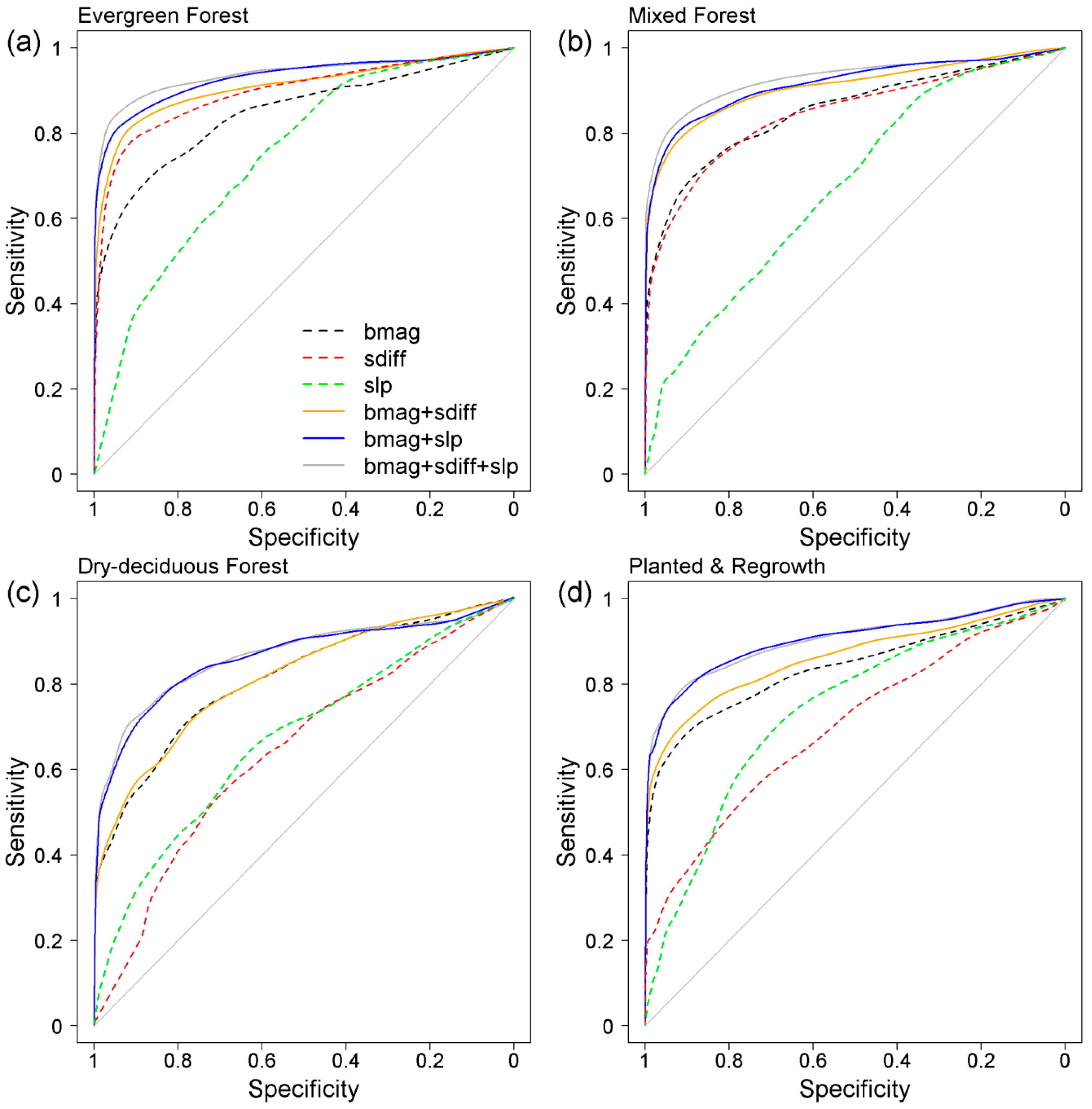
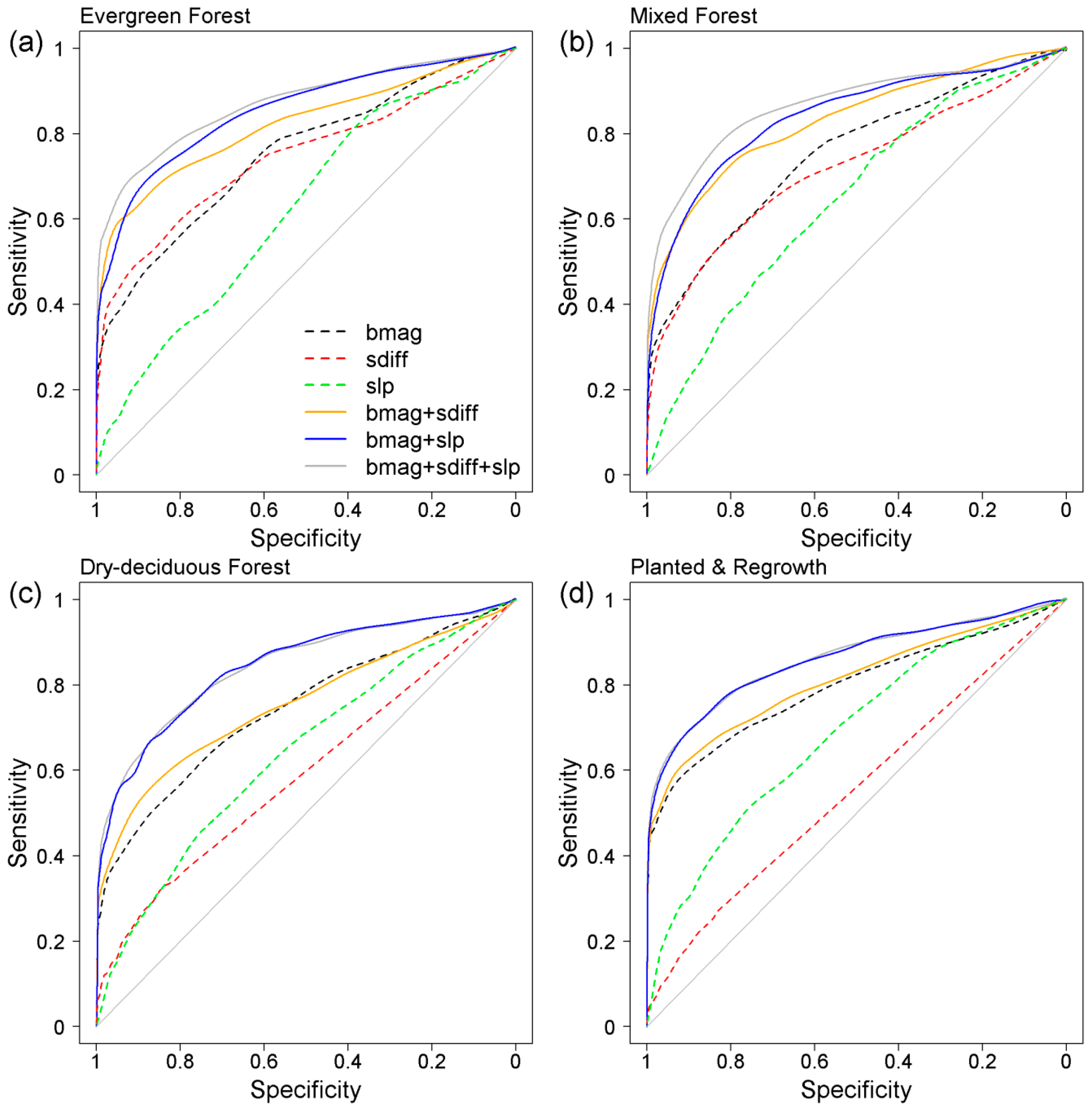
Appendix C. ROC Curves for MARS Models Using NDVI and EVI

C1. ROC Curves for MARS Models Using NDVI

Figure C1. Receiver operating characteristic (ROC) curves for models using different explanatory variables and combinations of variables derived from NDVI time series. Panels represent forest type: evergreen forest (a); mixed forest (b); dry-deciduous forest (c); and planted forest and regrowth (d).
Remotesensing 08 00657 g013
Table C1. Area under curve (AUC) estimates for regression models using NDVI and different combinations of parameters, by forest type. AUCs for each model are derived using receiver operating characteristic (ROC) curves presented in Figure C1.
VariablesEvergreen ForestMixed ForestDeciduous ForestPlanted and Regrowth
bmag + sdiff + slp0.950.930.890.91
bmag + slp0.940.920.880.91
bmag + sdiff0.910.900.800.87
bmag0.830.830.800.84
sdiff0.900.830.610.69
slp0.730.670.680.73

C2. ROC Curves for MARS Models Using EVI

Figure C2. Receiver operating characteristic (ROC) curves for models using different explanatory variables and combinations of variables derived from EVI time series. Panels represent forest type: evergreen forest (a); mixed forest (b); dry-deciduous forest (c); and planted forest and regrowth (d).
Remotesensing 08 00657 g014
Table C2. Area under curve (AUC) estimates for regression models using EVI and different combinations of parameters, by forest type. AUCs for each model are derived using receiver operating characteristic (ROC) curves presented in Figure C2.
VariablesEvergreen ForestMixed ForestDeciduous ForestPlanted and Regrowth
bmag + sdiff + slp0.860.870.850.86
bmag + slp0.830.840.850.86
bmag + sdiff0.810.820.750.81
bmag0.720.730.730.79
sdiff0.740.710.590.55
slp0.600.630.650.67

Appendix D

Table D1. Forest clearance commission errors (CE) and omission errors (OE) for different forest types using forest-type specific models and the generalized forest model. The example presented chooses probability thresholds (P) with the goal of attaining a commission error of 0.10. Data for the table are illustrated in Figure 5 and Figure 6 in the main article. Errors and probabilities are rounded to two decimal places.
Forest-Type SpecificGeneralised Forest
CEOEPCEOEP
Evergreen Forest0.100.060.300.030.160.54
Mixed Forest0.100.120.460.070.16
Deciduous Forest0.100.320.640.190.23
Planted and Regrowth0.100.230.560.100.26
Overall 0.100.18 0.100.20
Table D2. Forest clearance commission errors (CE) and omission errors (OE) for different forest types using forest-type specific models and the generalized forest model. The example presented chooses probability thresholds (P) with the goal of attaining a commission error of 0.20. Data for the table are illustrated in Figure 5 and Figure 6 in the main article. Errors and probabilities are rounded to two decimal places.
Forest-Type SpecificGeneralised Forest
CEOEPCEOEP
Evergreen Forest0.200.030.090.050.090.29
Mixed Forest0.200.060.170.160.08
Deciduous Forest0.200.180.390.350.10
Planted and Regrowth0.200.120.340.190.17
Overall 0.200.10 0.200.11

References

  1. Gibson, L.; Lee, T.M.; Koh, L.P.; Brook, B.W.; Gardner, T.A.; Barlow, J.; Peres, C.A.; Bradshaw, C.J.A.; Laurance, W.F.; Lovejoy, T.E.; et al. Primary forests are irreplaceable for sustaining tropical biodiversity. Nature 2011, 478, 378–381. [Google Scholar] [CrossRef] [PubMed]
  2. Myers, N.; Mittermeier, R.A.; Mittermeier, C.G.; Da Fonseca, G.A.; Kent, J. Biodiversity hotspots for conservation priorities. Nature 2000, 403, 853–858. [Google Scholar] [CrossRef] [PubMed]
  3. Bruijnzeel, L.A. Hydrological functions of tropical forests: not seeing the soil for the trees? Agric. Ecosyst. Environ. 2004, 104. [Google Scholar] [CrossRef]
  4. Aragão, L.E.O.C. The rainforest’s water pump. Nature 2012, 489, 217–218. [Google Scholar] [PubMed]
  5. Numata, I.; Cochrane, M.A.; Souza, C.M., Jr.; Sales, M.H. Carbon emissions from deforestation and forest fragmentation in the Brazilian Amazon. Environ. Res. Lett. 2011, 6, 044003. [Google Scholar] [CrossRef]
  6. Pan, Y.; Birdsey, R.A.; Fang, Y.; Houghton, R.; Kauppi, P.E.; Kurz, W.A.; Phillips, O.L.; Shvidenko, A.; Lewis, S.L.; Canadell, J.G.; et al. A large and persistent carbon sink in the world’s forests. Science 2011, 333, 988–994. [Google Scholar] [CrossRef] [PubMed]
  7. Guo, L.B.; Gifford, R.M. Soil carbon stocks and land use change : A meta analysis. Glob. Chang. Biol. 2002, 8, 345–360. [Google Scholar] [CrossRef]
  8. Belward, A.S.; Skøien, J.O. Who launched what, when and why; trends in global land-cover observation capacity from civilian earth observation satellites. ISPRS J. Photogramm. Remote Sens. 2015, 103, 115–128. [Google Scholar] [CrossRef]
  9. Coppin, P.; Jonckheere, I.; Nackaerts, K.; Muys, B.; Lambin, E. Review ArticleDigital change detection methods in ecosystem monitoring: A review. Int. J. Remote Sens. 2004, 25, 1565–1596. [Google Scholar] [CrossRef]
  10. Lu, D.; Mausel, P.; Brondízio, E.; Moran, E. Change detection techniques. Int. J. Remote Sens. 2004, 25, 2365–2401. [Google Scholar] [CrossRef]
  11. Huang, C.; Goward, S.N.; Masek, J.G.; Thomas, N.; Zhu, Z.; Vogelmann, J.E. An automated approach for reconstructing recent forest disturbance history using dense Landsat time series stacks. Remote Sens. Environ. 2010, 114, 183–198. [Google Scholar] [CrossRef]
  12. Kennedy, R.E.; Yang, Z.; Cohen, W.B. Detecting trends in forest disturbance and recovery using yearly Landsat time series: 1. LandTrendr—Temporal segmentation algorithms. Remote Sens. Environ. 2010, 114, 2897–2910. [Google Scholar] [CrossRef]
  13. Verbesselt, J.; Hyndman, R.; Newnham, G.; Culvenor, D. Detecting trend and seasonal changes in satellite image time series. Remote Sens. Environ. 2010, 114, 106–115. [Google Scholar] [CrossRef]
  14. Zhu, Z.; Woodcock, C.E. Continuous change detection and classification of land cover using all available Landsat data. Remote Sens. Environ. 2014, 144, 152–171. [Google Scholar] [CrossRef]
  15. Sulla-Menashe, D.; Kennedy, R.E.; Yang, Z.; Braaten, J.; Krankina, O.N.; Friedl, M.A. Detecting forest disturbance in the Pacific Northwest from MODIS time series using temporal segmentation. Remote Sens. Environ. 2014, 151, 114–123. [Google Scholar] [CrossRef]
  16. Goodwin, N.R.; Coops, N.C.; Wulder, M.A.; Gillanders, S.; Schroeder, T.A.; Nelson, T. Estimation of insect infestation dynamics using a temporal sequence of Landsat data. Remote Sens. Environ. 2008, 112, 3680–3689. [Google Scholar] [CrossRef]
  17. Mildrexler, D.J.; Zhao, M.; Running, S.W. Testing a MODIS global disturbance index across North America. Remote Sens. Environ. 2009, 113, 2103–2117. [Google Scholar] [CrossRef]
  18. Coops, N.C.; Wulder, M.A.; Iwanicka, D. Large area monitoring with a MODIS-based Disturbance Index (DI) sensitive to annual and seasonal variations. Remote Sens. Environ. 2009, 113, 1250–1261. [Google Scholar] [CrossRef]
  19. Vogelmann, J.E.; Tolk, B.; Zhu, Z. Monitoring forest changes in the southwestern United States using multitemporal Landsat data. Remote Sens. Environ. 2009, 113, 1739–1748. [Google Scholar] [CrossRef]
  20. Hostert, P.; Röder, A.; Hill, J. Coupling spectral unmixing and trend analysis for monitoring of long-term vegetation dynamics in Mediterranean rangelands. Remote Sens. Environ. 2003, 87, 183–197. [Google Scholar] [CrossRef]
  21. Verbesselt, J.; Hyndman, R.; Zeileis, A.; Culvenor, D. Phenological change detection while accounting for abrupt and gradual trends in satellite image time series. Remote Sens. Environ. 2010, 114, 2970–2980. [Google Scholar] [CrossRef]
  22. DeVries, B.; Verbesselt, J.; Kooistra, L.; Herold, M. Robust monitoring of small-scale forest disturbances in a tropical montane forest using Landsat time series. Remote Sens. Environ. 2015, 161, 107–121. [Google Scholar] [CrossRef]
  23. Zhu, Z.; Woodcock, C.E.; Olofsson, P. Continuous monitoring of forest disturbance using all available Landsat imagery. Remote Sens. Environ. 2012, 122, 75–91. [Google Scholar] [CrossRef]
  24. De Jong, R.; Verbesselt, J.; Zeileis, A.; Schaepman, M. Shifts in global vegetation activity trends. Remote Sens. 2013, 5, 1117–1133. [Google Scholar] [CrossRef] [Green Version]
  25. Clark, M.L.; Aide, T.M.; Grau, H.R.; Riner, G. A scalable approach to mapping annual land cover at 250 m using MODIS time series data: A case study in the Dry Chaco ecoregion of South America. Remote Sens. Environ. 2010, 114, 2816–2832. [Google Scholar] [CrossRef]
  26. Hurni, K.; Hett, C.; Heinimann, A.; Messerli, P.; Wiesmann, U. Dynamics of shifting cultivation landscapes in Northern Lao PDR between 2000 and 2009 based on an analysis of MODIS time series and Landsat images. Hum. Ecol. 2012, 41, 21–36. [Google Scholar] [CrossRef]
  27. Fensholt, R.; Horion, S.; Tagesson, T.; Ehammer, A.; Ivits, E.; Rasmussen, K. Global-scale mapping of changes in ecosystem functioning from earth observation-based trends in total and recurrent vegetation. Glob. Ecol. Biogeogr. 2015, 24, 1003–1017. [Google Scholar] [CrossRef]
  28. Koltunov, A.; Ustin, S.L.; Asner, G.P.; Fung, I. Selective logging changes forest phenology in the Brazilian Amazon: Evidence from MODIS image time series analysis. Remote Sens. Environ. 2009, 113, 2431–2440. [Google Scholar] [CrossRef]
  29. Boschetti, L.; Flasse, S.P.; Brivio, P.A. Analysis of the conflict between omission and commission in low spatial resolution dichotomic thematic products: The Pareto Boundary. Remote Sens. Environ. 2004, 91, 280–292. [Google Scholar] [CrossRef]
  30. Morton, D.C.; DeFries, R.S.; Shimabukuro, Y.E.; Anderson, L.O.; Del Bon Espírito-Santo, F.; Hansen, M.; Carroll, M. Rapid assessment of annual deforestation in the brazilian amazon using MODIS data. Earth Interact. 2005, 9, 1–22. [Google Scholar] [CrossRef]
  31. Gutiérrez-Vélez, V.H.; DeFries, R. Annual multi-resolution detection of land cover conversion to oil palm in the Peruvian Amazon. Remote Sens. Environ. 2013, 129, 154–167. [Google Scholar] [CrossRef]
  32. Langner, A.; Miettinen, J.; Siegert, F. Land cover change 2002–2005 in Borneo and the role of fire derived from MODIS imagery. Glob. Chang. Biol. 2007, 13, 2329–2340. [Google Scholar] [CrossRef]
  33. Hansen, M.C.; Stehman, S.V.; Potapov, P.V.; Loveland, T.R.; Townshend, J.R.G.; Defries, R.S.; Pittman, K.W.; Arunarwati, B.; Stolle, F.; Steininger, M.K.; et al. Humid tropical forest clearing from 2000 to 2005 quantified by using multitemporal and multiresolution remotely sensed data. Proc. Natl. Acad. Sci. USA 2008, 105, 9439–9444. [Google Scholar] [PubMed]
  34. Broich, M.; Stehman, S.V.; Hansen, M.C.; Potapov, P.; Shimabukuro, Y.E. A comparison of sampling designs for estimating deforestation from Landsat imagery: A case study of the Brazilian Legal Amazon. Remote Sens. Environ. 2009, 113, 2448–2454. [Google Scholar] [CrossRef]
  35. Shimabukuro, Y.E.; Duarte, V.; Anderson, L.O.; Valeriano, D.M.; Arai, E.; Freitas, R.M.; Rudorff, B.F.T.; Moreira, M.A. Near real time detection of deforestation in the Brazilian Amazon using MODIS imagery. Ambient. e Água—Interdiscip. J. Appl. Sci. 2006, 1, 37–47. [Google Scholar] [CrossRef]
  36. Spruce, J.P.; Sader, S.; Ryan, R.E.; Smoot, J.; Kuper, P.; Ross, K.; Prados, D.; Russell, J.; Gasser, G.; McKellip, R. Assessment of MODIS NDVI time series data products for detecting forest defoliation by GYPSY moth outbreaks. Remote Sens. Environ. 2011, 115, 427–437. [Google Scholar] [CrossRef]
  37. Xin, Q.; Olofsson, P.; Zhu, Z.; Tan, B.; Woodcock, C.E. Toward near real-time monitoring of forest disturbance by fusion of MODIS and Landsat data. Remote Sens. Environ. 2013, 135, 234–247. [Google Scholar] [CrossRef]
  38. Verbesselt, J.; Zeileis, A.; Herold, M. Near real-time disturbance detection using satellite image time series. Remote Sens. Environ. 2012, 123, 98–108. [Google Scholar] [CrossRef]
  39. Broich, M.; Hansen, M.C.; Potapov, P.; Adusei, B.; Lindquist, E.; Stehman, S.V. Time-series analysis of multi-resolution optical imagery for quantifying forest cover loss in Sumatra and Kalimantan, Indonesia. Int. J. Appl. Earth Obs. Geoinf. 2011, 13, 277–291. [Google Scholar] [CrossRef]
  40. Hostert, P.; Griffiths, P.; Van Der Linden, S.; Pflugmacher, D. Time series analyses in a new era of optical satellite data. In Remote Sensing Time Series; Kuenzer, C., Dech, S., Wagner, W., Eds.; Springer International Publishing: Gewerbestrasse, Switzerland, 2015; Volume 22, pp. 25–41. [Google Scholar]
  41. Wulder, M.A.; Masek, J.G.; Cohen, W.B.; Loveland, T.R.; Woodcock, C.E. Opening the archive: How free data has enabled the science and monitoring promise of Landsat. Remote Sens. Environ. 2012, 122, 2–10. [Google Scholar] [CrossRef]
  42. Griffiths, P.; Kuemmerle, T.; Kennedy, R.E.; Abrudan, I.V.; Knorn, J.; Hostert, P. Using annual time-series of Landsat images to assess the effects of forest restitution in post-socialist Romania. Remote Sens. Environ. 2012, 118, 199–214. [Google Scholar] [CrossRef]
  43. Masek, J.G.; Huang, C.; Wolfe, R.; Cohen, W.; Hall, F.; Kutler, J.; Nelson, P. North American forest disturbance mapped from a decadal Landsat record. Remote Sens. Environ. 2008, 112, 2914–2926. [Google Scholar] [CrossRef]
  44. Walston, J.; Davidson, P.; Soriyun, M. A wildlife survey of Southern Mondulkiri province, Cambodia. Cildlife Conserv. Soc. Cambodia Progr. 2001. [Google Scholar]
  45. Grogan, K.; Pflugmacher, D.; Hostert, P.; Kennedy, R.; Fensholt, R. Cross-border forest disturbance and the role of natural rubber in mainland Southeast Asia using annual Landsat time series. Remote Sens. Environ. 2015, 169, 438–453. [Google Scholar] [CrossRef]
  46. Tucker, C.J. Red and photographic infrared linear combinations for monitoring vegetation. Remote Sens. Environ. 1979, 150, 127–150. [Google Scholar] [CrossRef]
  47. Huete, A.; Didan, K.; Miura, T.; Rodriguez, E.P.; Gao, X.; Ferreira, L.G. Overview of the radiometric and biophysical performance of the MODIS vegetation indices. Remote Sens. Environ. 2002, 83, 195–213. [Google Scholar] [CrossRef]
  48. Boles, S.H.; Xiao, X.; Liu, J.; Zhang, Q.; Munkhtuya, S.; Chen, S.; Ojima, D. Land cover characterization of Temperate East Asia using multi-temporal VEGETATION sensor data. Remote Sens. Environ. 2004, 90, 477–489. [Google Scholar] [CrossRef]
  49. Xiao, X.; Biradar, C.M.; Czarnecki, C.; Alabi, T.; Keller, M. A simple algorithm for large-scale mapping of evergreen forests in tropical America, Africa and Asia. Remote Sens. 2009, 1, 355–374. [Google Scholar] [CrossRef]
  50. Bai, J.; Perron, P. Computation and analysis of multiple structural change models. J. Appl. Econ. 2003, 18, 1–22. [Google Scholar] [CrossRef]
  51. Sexton, J.O.; Song, X.P.; Feng, M.; Noojipady, P.; Anand, A.; Huang, C.; Kim, D.H.; Collins, K.M.; Channan, S.; DiMiceli, C.; Townshend, J.R. Global, 30-m resolution continuous fields of tree cover: Landsat-based rescaling of MODIS vegetation continuous fields with lidar-based estimates of error. Int. J. Digit. Earth 2013, 6, 427–448. [Google Scholar] [CrossRef]
  52. Global Land Cover 2000 Legend. Available online: http://forobs.jrc.ec.europa.eu/products/glc2000/legend.php (accessed on 1 July 2016).
  53. Breiman, L. Random forests. Mach. Learn. 2001, 45, 5–32. [Google Scholar] [CrossRef]
  54. Cohen, W.B.; Yang, Z.; Kennedy, R. Detecting trends in forest disturbance and recovery using yearly Landsat time series: 2. TimeSync—Tools for calibration and validation. Remote Sens. Environ. 2010, 114, 2911–2924. [Google Scholar] [CrossRef]
  55. Friedman, J.H. Multivariate adaptive regression splines. Ann. Stat. 1991, 19, 1–67. [Google Scholar] [CrossRef]
  56. Hastie, T.; Tibshirani, R.; Friedman, J. The Elements of Statistical Learning. Data Mining, Inference, and Prediction, 2nd ed.; Springer: New York, NY, USA, 2009. [Google Scholar]
  57. Couturier, S. A fuzzy-based method for the regional validation of global maps: The case of MODIS-derived phenological classes in a mega-diverse zone. Int. J. Remote Sens. 2010, 31, 5797–5811. [Google Scholar] [CrossRef]
  58. La Barreda-Bautista, B.D.; López-Caloca, A.A.; Couturier, S.; Silván-Cárdenas, J.L. Tropical dry forests in the GLOBAL Picture : The challenge of remote sensing-based change detection in tropical dry environments. In Planet Earth 2011—Global Warming Challenges and Opportunities for Policy and Practice; INTECH Open Access Publisher: Rijeka, Croatia, 2011; pp. 231–256. [Google Scholar]
  59. Stibig, H.J.; Achard, F.; Carboni, S.; Raši, R.; Miettinen, J. Change in tropical forest cover of Southeast Asia from 1990 to 2010. Biogeosciences 2014, 11, 247–258. [Google Scholar] [CrossRef] [Green Version]
  60. Castro-Esau, K.L.; Kalacska, M. Tropical Dry Forest Phenology and Discrimination of Tropical Tree Species Using Hyperspectral Data. In Hyperspectral Remote Sensing of Tropical and Sub-Tropical Forests; Kalacska, M., Sanchez-Azofeifa, G.A., Eds.; CRC Press: Boca Raton, FL, USA, 2008; pp. 1–26. [Google Scholar]
  61. Borchert, R. Soil and stem water storage determine phenology and distribution of tropical dry forest Trees. Ecology 1994, 75, 1437–1449. [Google Scholar] [CrossRef]
  62. Williams, L.J.; Bunyavejchewin, S.; Baker, P.J. Deciduousness in a seasonal tropical forest in western Thailand: Interannual and intraspecific variation in timing, duration and environmental cues. Oecologia 2008, 155, 571–582. [Google Scholar] [CrossRef] [PubMed]
  63. Yoshifuji, N.; Kumagai, T.; Tanaka, K.; Tanaka, N.; Komatsu, H.; Suzuki, M.; Tantasirin, C. Inter-annual variation in growing season length of a tropical seasonal forest in northern Thailand. For. Ecol. Manag. 2006, 229, 333–339. [Google Scholar] [CrossRef]
  64. Jamali, S.; Jönsson, P.; Eklundh, L.; Ardö, J.; Seaquist, J. Detecting changes in vegetation trends using time series segmentation. Remote Sens. Environ. 2015, 156, 182–195. [Google Scholar] [CrossRef]
  65. Dutrieux, L.P.; Verbesselt, J.; Kooistra, L.; Herold, M. Monitoring forest cover loss using multiple data streams, a case study of a tropical dry forest in Bolivia. ISPRS J. Photogramm. Remote Sens. 2015, 107, 112–125. [Google Scholar] [CrossRef]
  66. Healey, S.P.; Yang, Z.; Cohen, W.B.; Pierce, D.J. Application of two regression-based methods to estimate the effects of partial harvest on forest structure using Landsat data. Remote Sens. Environ. 2006, 101, 115–126. [Google Scholar] [CrossRef]
  67. Wilson, E.H.; Sader, S.A. Detection of forest harvest type using multiple dates of Landsat TM imagery. Remote Sens. Environ. 2002, 80, 385–396. [Google Scholar] [CrossRef]
  68. Hais, M.; Jonášová, M.; Langhammer, J.; Kučera, T. Comparison of two types of forest disturbance using multitemporal Landsat TM/ETM+ imagery and field vegetation data. Remote Sens. Environ. 2009, 113, 835–845. [Google Scholar] [CrossRef]
  69. Song, C.; Woodcock, C.E. Monitoring forest succession with multitemporal landsat images: factors of uncertainty. IEEE Trans. Geosci. Remote Sens. 2003, 41, 2557–2567. [Google Scholar] [CrossRef]
  70. Czerwinski, C.J.; King, D.J.; Mitchell, S.W. Mapping forest growth and decline in a temperate mixed forest using temporal trend analysis of Landsat imagery, 1987–2010. Remote Sens. Environ. 2014, 141, 188–200. [Google Scholar] [CrossRef]
  71. Schmidt, M.; Lucas, R.; Bunting, P.; Verbesselt, J.; Armston, J. Multi-resolution time series imagery for forest disturbance and regrowth monitoring in Queensland, Australia. Remote Sens. Environ. 2015, 158, 156–168. [Google Scholar] [CrossRef] [Green Version]
  72. DeVries, B.; Decuyper, M.; Verbesselt, J.; Zeileis, A.; Herold, M.; Joseph, S. Tracking disturbance-regrowth dynamics in tropical forests using structural change detection and Landsat time series. Remote Sens. Environ. 2015, 169, 320–334. [Google Scholar] [CrossRef]
  73. Grogan, K.; Fensholt, R. Exploring patterns and effects of aerosol quantity flag anomalies in MODIS surface reflectance products in the tropics. Remote Sens. 2013, 5, 3495–3515. [Google Scholar] [CrossRef]
  74. Leinenkugel, P.; Kuenzer, C.; Dech, S. Comparison and enhancement of MODIS cloud mask products for Southeast Asia. Int. J. Remote Sens. 2013, 34, 2730–2748. [Google Scholar] [CrossRef]
  75. Hilker, T.; Lyapustin, A.I.; Tucker, C.J.; Sellers, P.J.; Hall, F.G.; Wang, Y. Remote sensing of tropical ecosystems: Atmospheric correction and cloud masking matter. Remote Sens. Environ. 2012, 127, 370–384. [Google Scholar] [CrossRef]
  76. Lambin, E.F.; Ehrlich, D. Land-cover changes in Sub-Saharan Africa (1982–1991): Application of a change index based on remotely sensed surface temperature and vegetation indices at a continental scale. Remote Sens. Environ. 1997, 61, 181–200. [Google Scholar] [CrossRef]
  77. Lambin, E.F.; Geist, H.J.; Lepers, E. Dynamics of Land-Use and land-cover change tropics regions. Annu. Rev. Environ. Resour. 2003, 28, 205–241. [Google Scholar] [CrossRef]
  78. Jamali, S.; Seaquist, J.; Eklundh, L.; Ardö, J. Automated mapping of vegetation trends with polynomials using NDVI imagery over the Sahel. Remote Sens. Environ. 2014, 141, 79–89. [Google Scholar] [CrossRef]
  79. Achard, F.; Boschetti, L.; Brown, S.; Brady, M.; DeFries, R.; Grassi, G.; Herold, M.; Mollicone, D.; Mora, B.; Pandey, D.; et al. A Sourcebook of Methods and Procedures for Monitoring and Reporting Anthropogenic Greenhouse Gas Emissions and Removals Caused by Deforestation, Gains and Losses of Carbon Stocks in Forests Remaining Forests, and Forestation; GOFC-GOLD: Wageningen, The Netherlands, 2014. [Google Scholar]
  80. Potapov, P.; Hansen, M.C.; Stehman, S.V.; Loveland, T.R.; Pittman, K. Combining MODIS and Landsat imagery to estimate and map boreal forest cover loss. Remote Sens. Environ. 2008, 112, 3708–3719. [Google Scholar] [CrossRef]
  81. Dymond, J.R.; Shepherd, J.D.; Arnold, G.C.; Trotter, C.M. Estimating area of forest change by random sampling of change strata mapped using satellite imagery. For. Sci. 2008, 54, 475–480. [Google Scholar]
  82. McRoberts, R.E.; Walters, B.F. Statistical inference for remote sensing-based estimates of net deforestation. Remote Sens. Environ. 2012, 124, 394–401. [Google Scholar] [CrossRef]
  83. Wilson, A.M.; Parmentier, B.; Jetz, W. Systematic land cover bias in Collection 5 MODIS cloud mask and derived products—A global overview. Remote Sens. Environ. 2014, 141, 149–154. [Google Scholar] [CrossRef]
  84. Liu, R.; Liu, Y. Generation of new cloud masks from MODIS land surface reflectance products. Remote Sens. Environ. 2013, 133, 21–37. [Google Scholar] [CrossRef]
  85. Jönsson, P.; Eklundh, L. TIMESAT—A program for analyzing time-series of satellite sensor data. Comput. Geosci. 2004, 30, 833–845. [Google Scholar] [CrossRef]
  86. Dong, J.; Xiao, X.; Chen, B.; Torbick, N.; Jin, C.; Zhang, G.; Biradar, C. Mapping deciduous rubber plantations through integration of PALSAR and multi-temporal Landsat imagery. Remote Sens. Environ. 2013, 134, 392–402. [Google Scholar] [CrossRef]
Figure 1. Study area map with forest cover for year 2000. See Section 3.3 for details of forest classification.
Remotesensing 08 00657 g001
Figure 2. Examples of Breaks For Additive Season and Trend (BFAST) and three change indicator variables. Simulated 16-day composite data with breakpoints at year 2006 were used for this methodological description showing: the break magnitude (bmag) (a); the seasonal amplitude difference (sdiff) (b); and the most negative slope (slp) of the first (slp1) and second (slp2) trend segment—in the example presented this is slp2 (c).
Remotesensing 08 00657 g002
Figure 3. Examples of Breaks For Additive Season and Trend (BFAST) output using the Land Surface Water Index (LSWI) time series: (a) evergreen forest; (b) mixed forest; (c) dry-deciduous forest; and (d) rubber plantation. The panels to the right of each plot include true colour Landsat imagery for selected years before and after the detected forest clearance. The MODIS pixels used for each example are shown by the centred white and red outlines. For the plots, light grey = original time series, blue = fitted trend model, and black = fitted seasonal model.
Remotesensing 08 00657 g003
Figure 4. Receiver operating characteristic (ROC) curves for models using different explanatory variables and combinations of variables. Panels represent forest type: evergreen forest (a); mixed forest (b); dry-deciduous forest (c); and planter forest and regrowth (d). The variable combination bmag + sdiff + slp was omitted from the plots as it closely resembled the curve of bmag + slp.
Remotesensing 08 00657 g004
Figure 5. Forest clearance commission Vs omission errors for: the forest-type specific models (a); and the generalised forest model (b). All models presented used the bmag + slp variable combination. Points where errors are balanced follow the 1:1 dashed line. Predicted probabilities for each model are shown as additional x-axes using the same colour scheme. Points marked on the predicted probability axes are at thresholds where errors area balanced.
Remotesensing 08 00657 g005
Figure 6. Overall forest clearance commission (a) and omission (b) errors using the generalised forest model (GM) and how this error is distributed among the four forest types within the generalised model (FT-GM). Error rates for the generalised model are shown on the x-axes, and are an average of error within each forest type shown on y-axes. The vertical dashed line represents the point where overall error for the generalised model is balanced at 0.15. The generalised model’s predicted probability of clearance is provided as an additional x-axis, and marked at a threshold where the overall error is balanced.
Remotesensing 08 00657 g006
Figure 7. Comparison of Landsat reference map and MODIS forest clearance map using the bmag + slp forest-type specific models, and Land Surface Water Index (LSWI) time series. Landsat imagery (RGB = bands 3, 2, and 1) from year 2000 and 2012 are shown for three study area subsets showing; clearing in evergreen forest by mostly smallholders (a); large-scale clearing of evergreen forest for plantations (b); and clearing of evergreen, mixed and dry-deciduous forest (c).
Remotesensing 08 00657 g007
Figure 8. Sensitivity of the Land Surface Water Index (LSWI) change model to sub-pixel clearance by forest type: evergreen forest (a); mixed forest (b); dry-deciduous forest (c); and planted forest and regrowth (d) Histograms of forest clearance omission error using pixel cleared proportion (Cp) intervals of 10% were made using the validation samples. Results represent sub-pixel omission errors using a probability threshold where forest clearance commission and omission error are balanced.
Remotesensing 08 00657 g008
Figure 9. Agreement between clearance timing from the validation sample and the BFAST clearance timing using MODIS Land Surface Water Index (LSWI). Each bar represents a stratum of the validation sample based on the number of clearances that occurred within MODIS pixel samples. Agreement was assessed using two methods: (1) year of the greatest cleared proportion (Greatest Cp); and (2) year of the first forest clearance (First Cp). Often the clearance timing label was both the greatest and first clearance (Greatest and First Cp).
Remotesensing 08 00657 g009
Table 1. Area under curve (AUC) estimates for regression models using different parameters and combinations of parameters, by forest type. AUCs for all models are derived using receiver operating characteristic (ROC) curves presented in Figure 4.
VariablesEvergreen ForestMixed ForestDeciduous ForestPlanted and Regrowth
bmag + sdiff + slp0.980.960.890.92
bmag + slp0.970.960.890.92
bmag + sdiff0.960.940.790.87
bmag0.930.900.780.83
sdiff0.940.860.610.72
slp0.790.700.680.74
Table 2. Forest clearance commission errors (CE) and omission errors (OE) for different forest types using forest-type specific models and the generalised forest model. The example presented chooses probability thresholds (P) with the goal of balancing commission and omission error. Data for the table are illustrated as points in Figure 5 and Figure 6. Errors and probabilities are rounded to two decimal places.
Forest-Type SpecificGeneralised Forest
CEOEPCEOEP
Evergreen Forest0.080.080.350.040.130.40
Mixed Forest0.110.110.410.100.11
Deciduous Forest0.190.190.400.280.14
Planted and Regrowth0.160.160.420.140.21
Overall 0.140.14 0.150.15

