1. Introduction
In the last few decades, there has been a strong legislative effort to improve the quality of freshwater ecosystems at both European and international level [
1,
2]. Within Europe, the Water Framework Directive [
3] dictates the parameters to be monitored for the assessment of the ecological status of a given water body, where a water body is the basic unit used to assess the quality of the water environment and used as reference for environmental improvements. The ecological quality parameters sampled draw upon five different domains: biological, physico-chemical, chemical, specific pollutants and supporting elements [
3]. In the particular case of supporting elements, hydromorphology plays a key role in the assessment of hydrology (i.e., quantity and dynamics of water flow and connection to groundwater bodies), morphology (i.e., river depth and width variation, structure and substrate of the river and structure of the riparian zone) and river continuity [
4]. Hydromorphological characterisation has also been recognised to be key for river management and restoration [
5,
6] and essential in the understanding of biological metrics [
6,
7].
The list of methods available to assess hydromorphology for regulatory purposes is vast and varied. Belletti et al. [
4] compared over 100 EU hydromorphological assessment methods and classified them in four broad categories based on the key features surveyed: physical habitat, riparian habitat, morphological and hydrological regime alteration. The majority of methods compared rely on physical habitat identification and require the recognition of in-channel features that define homogenous areas of flow, vegetation and substrate [
8] from either aerial imagery (e.g., [
9]) or extensive field based work (e.g., [
10,
11]). An example is the UK assessment of flow types describing the lentic-lotic character of a reach that is routinely used at a National scale to assess river quality [
7,
8,
12]. For aerial imagery based methods, the success of feature identification relies heavily on the resolution of the imagery used [
13]. High resolution remote sensing products are expected to provide better feature identification accuracy than imagery commercially available. This has been proved true by several authors in a range of different research disciplines [
14,
15,
16,
17]. However, some of the approaches used to compare the accuracy in feature identification rely on resolutions obtained by averaging adjacent pixels from a ground truth orthoimage captured at fine resolution [
16]. These approaches are incomplete as they fail to take into account the uncertainty arising from differing flight planning parameters (e.g., number of frames, flying heights, image footprint) required to obtain the desired geomatic products. Methods that contrast metrics derived from remote sensing products that have been obtained from data captured at different resolutions [
15,
18] should therefore be preferred. This is particularly relevant in river research projects where unmanned aerial vehicles (UAVs) are being used to capture high resolution aerial imagery for automated feature identification [
19,
20]. These automated classification techniques based on either object-based image analysis, unsupervised or supervised methods [
21] provide feature identification results that match those obtained through visual based approaches and have been suggested as potential cost-effective approaches to satisfy national scale river hydromorphological assessment requirements [
9,
19].
Generally, coarse resolution imagery (12 cm–25 cm) has been used for the purposes outlined above. The imagery is captured through manned aircrafts that are able to cover wide areas using standard remote sensing cameras. Higher resolution imagery can be obtained with aircrafts equipped with more specialised and expensive equipment, with the highest resolution (finer than 1 cm) being obtained from either rotary or fixed wing UAVs [
14,
22]. The imagery resolution from aircrafts and UAVs is the result of a combination of both camera specifications and pre-selected flying height [
17,
23].
The choice between aircraft and UAVs depends upon the capability of the platform to integrate sensor requirements (e.g., camera payload—see [
24] for a review) followed by the cost-effectiveness (low weight, slow flight, speed and extended range) and safety of the overall mission. From a financial perspective, fuel consumption is generally the limiting factor for aircraft deployment whereas local deployment of UAVs are cost-effective methods for timely and on-demand data collection when considering platform acquisition at fixed cost [
22]. From a safety perspective, aircrafts are more stable than UAVs, in particular under gusty and wet conditions, and do not present drawbacks for flights planned over congested areas. UAV reliability when in flight is still a safety concern although recent platforms incorporate a set of failsafe options that ensure the recovery of the UAV in emergency situations (e.g., GPS failure). Both aircrafts and UAVs require compliance with national and international airspace regulatory frameworks, which currently are not standardised between countries for UAV usage. In terms of data acquisition, UAVs are able to fly under cloud cover and, although limited by battery life endurance and visual line of sight (500 m) regulatory constraints, enable data capture at higher resolutions than aircraft alternatives. UAV platforms range from inexpensive and light options such as blimps, kites or balloons to more sophisticated and expensive vertical take-off-and-landing (VTOL) and fixed wing platforms. VTOLs and fixed wings are preferred over light options due to their better manoeuvrability [
22]. The selection of a specific UAV platform depends on the capability of its gimbal to integrate the payload; the extension of the survey area to be covered as well as deployment and flight plan logistics. VTOL UAVs are able to hover over a point and provide high resolution still imagery whereas fixed wing platforms enable wide area surveying [
22].
Rapid advances in technology suggest that UAVs will be the preferred option for environmental data collection in the not too distant future [
14]. For example, Sankaran et al. [
25] identified UAVs as a low-cost, rapid and flexible alternative to airborne LIDAR for geomorphological mapping in general and highlights the added benefit of using UAVs to test models, forecast and understand the evolution of environmental processes; and Woodget et al. [
26] believes that photogrammetric methodologies based on high resolution UAV aerial imagery could become the tool of choice for routine and reliable assessment of physical river habitat in the future. Within this context, little effort has been made to assess the added benefit of using UAV high resolution aerial imagery for hydromorphological assessment. In particular, whether the expected increase in feature identification accuracy justifies the use of UAV high resolution aerial imagery. Previous work has focused on the effect of spatial (i.e., 1 m and 2.5 m pixel sixe), spectral (i.e., hyper- and multi-spectral) and radiometric (i.e., 8 bit and 11 bit) resolution on the identification of in-stream habitats by comparing hyperspectral imagery to simulated multispectral data [
27]. In [
27], the spectral resolution was more relevant than the spatial or radiometric resolution for the automated identification of in-channel features (riffles, glides, pools and eddy drop zones). Anker et al. [
28] focused on the effectiveness of aerial digital photography-spectral analysis (ADP-SP) to assess macrophyte cover when compared to ground-level data and hyperspectral imagery. ADP-SP presented a better spatial resolution than ground-level and hyperspectral data (4 cm vs. 1 m and 10 cm) and enabled the differentiation between emergent and submerged vegetation. In [
29], the effectiveness of digital airborne imagery at two different resolutions (3 cm and 10 cm) to estimate median surface grain sizes were compared. The study showed that 10 cm resolution imagery was unsuitable for grain size estimation.
Here, we contrast a total of three orthoimages derived from UAV high resolution aerial imagery physically obtained for this intention. The aim is to quantify the uncertainty in automated river hydromorphological feature identification when using aerial imagery of different resolutions (i.e., 2.5 cm, 5 cm and 10 cm). This work builds on previous research carried out by the authors [
19] on the development of a framework for the integration of UAV high resolution imagery and Artificial Neural Networks (ANNs) for the automatic classification of hydromorphological features. This framework has been shown to identify hydromorphological features with an averaged success rate of over 81% and will be used to address the aim of his paper through the following three interdependent objectives:
- 1
To quantify the performance of an ANN based operational framework [
19] for hydromorphological feature identification at different aerial imagery resolutions.
- 2
To identify the optimal aerial imagery resolution required for robust automated hydromorphological assessment.
- 3
To assess the implications of results obtained from (1) and (2) in a regulatory context.
3. Results
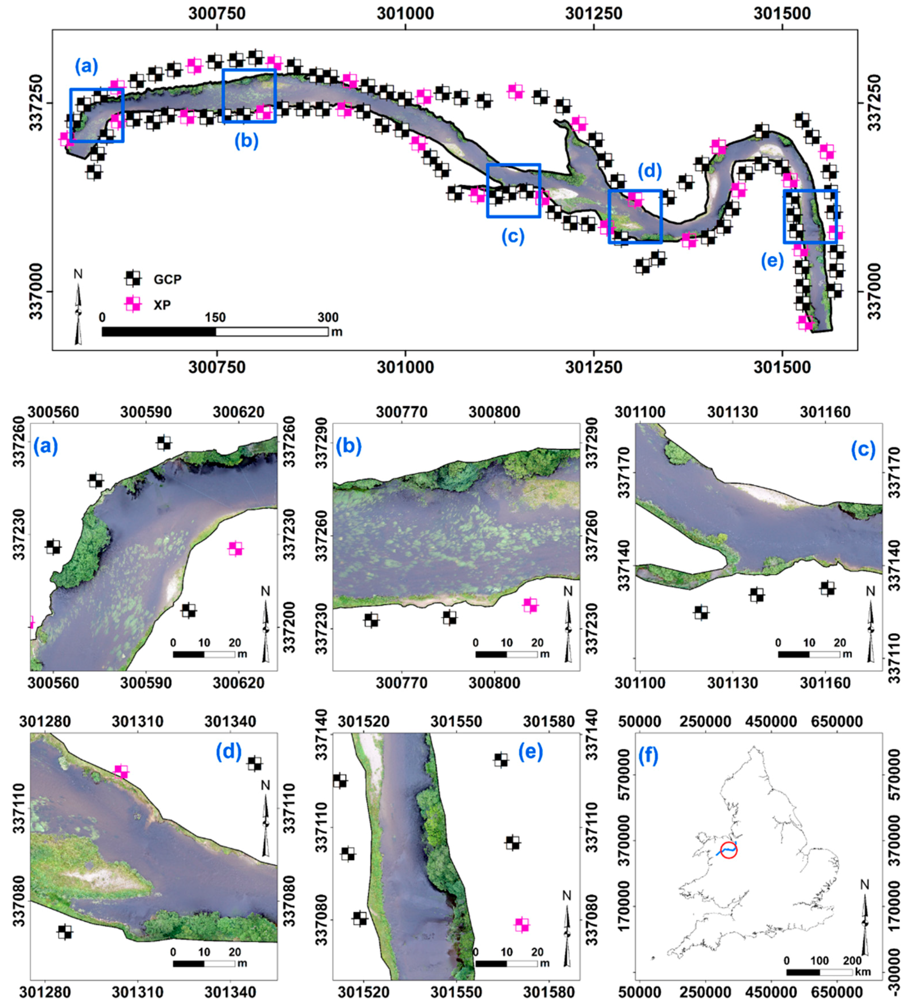
The coregistration errors for the GCPs increase in
x,
y and
z as the imagery resolution coarsens, with errors below 3 cm for the finer resolutions and up to 31 cm for the coarser resolution. A similar pattern is observed for the XPs, where the coregistration error in
x,
y and
z reaches values of nearly 3 cm for the orthoimage at 2.5 cm resolution and up to 83 cm for the coarser resolution. The increase in coregistration error is more evident when estimating the RMSE, which is ≈4.5 cm for the finer scales but larger than 3 m for the 10 cm resolution orthoimage (
Table 3). The elapsed time required to process the imagery to obtain the geomatic products decreases as the resolution coarsens because the number of frames to be processed diminishes (
Table 3). Here, the elapsed time refers to the time required by the computer to generate the geomatic products based on the performance of a computer with an Intel Core i7-5820 K 3.30 GHz processor, 32 Gb RAM and 2 graphic cards (NVIDIA Geoforce GTZ 980 and NVDIA Qadro K2200). An extra 7 h, 5.5 h and 3 h were required to locate the GCPs manually for the imagery at 2.5 cm, 5 cm and 10 cm resolution, respectively.
The total accuracy (
AC) in automated feature classification is ≈65%, with a slight decrease in feature identification power as the resolution coarsens (
Table 4). LAIC enables the allocation of multiple classification to a given point or pixel. For example, a given point falling in an area where both riffles and submerged vegetation are present will be simultaneously classified under feature classes riffle and vegetation. If the effect of multiple classification is taken into account, the overall accuracy ranges between 67% (at 10 cm resolution) and 76% (at 2.5 cm resolution) (
Table 4). These results are consistent with those obtained for the
k-statistic, which shows that at 2.5 cm resolution the classification is good but deteriorates down to fair and poor [
36] for 5 cm and 10 cm resolutions, respectively. The measures of disagreement
C and
Q show that the disagreement between the ground truth point data set and the classifications obtained for each of the three resolutions is primarily due to the spatial allocation of feature classes (
Q) rather than the proportion (
C) represented by each class (
Figure 4).
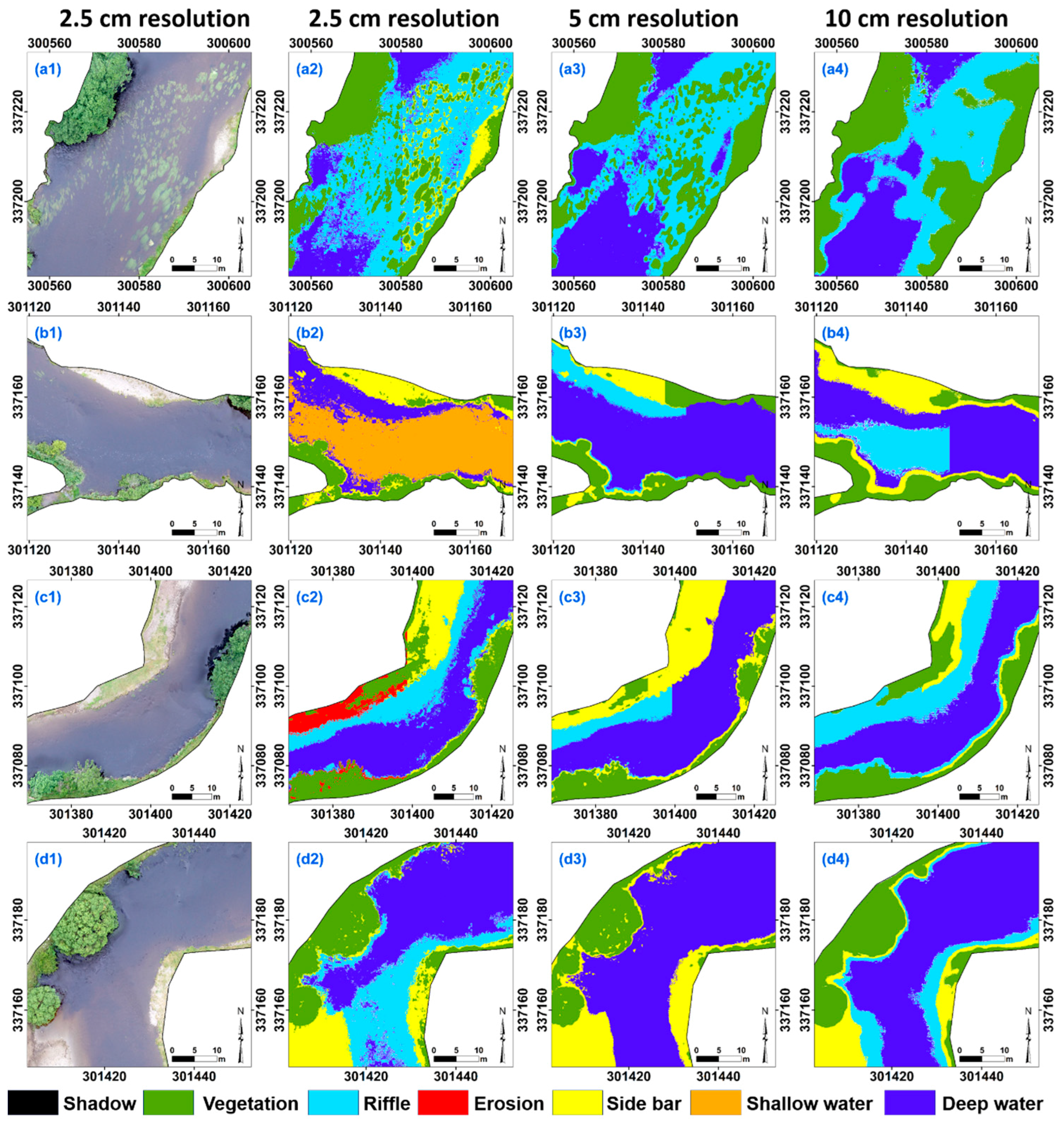
At feature level, the performance in classification measured through
TPR and
TNR (
Table 5) decreases as the resolution coarsens for side bars, riffles and vegetation. Both, shadows and erosion are only detectable at 2.5 cm resolution (
Figure 4) and omitted from the classifications obtained at coarser resolutions. For deep and shallow water, the pattern of change with resolution is not as clear or relevant as for the other feature classes.
When multiple classification is taken into account, the power in feature identification increases for riffles, deep waters and shallow waters, with some of the features reaching
TPR values larger than 94% (
Table 5). The ratio of single, double and triple feature allocations at 2.5 cm, 5 cm and 10 cm resolution are 10,360, 453 and 6; 10,420, 436 and 2; and 10,629, 205 and 1, respectively. The power to detect multiple classifications is larger at finer resolutions than at coarser ones. For example, at 2.5 cm resolution, LAIC is able to identify points with submerged vegetation present within riffle and shallow water categories, whereas this ability disappears at 10 cm resolution where submerged vegetation and riffles are barely identifiable (
Figure 4). At 2.5 cm and 5 cm resolution, the number of double classifications assigned is comparable (453 and 436, respectively). However, at 10 cm resolution the value plummets down to 205. The most frequent combinations of double classification occur in the forms: (i) shallow water with deep water (162, 292, and 104 points for each of the three resolutions from finer to coarser); and (ii) shallow water with riffle (94, 58, and 36 points). Triple classifications are sporadic at all resolutions considered.
The
FNR value (
Table 5) increases as the resolution coarsens, reaching values of 100% for erosion and shadow. The large
FNR values indicate that these features fail to be identified at resolutions coarser than 2.5 cm. The
FNR for riffles increases from 53% to 87% from finer resolution to coarser, whereas the
FPR value for deep and shallow water increases as resolution coarsens. This is because riffle features get systematically replaced by shallow and deep water classifications when the imagery resolution coarsens. A similar pattern is observed for side bars, for which
FNR increases from 14% at 2.5 cm resolution to 99% at 10 cm resolutions.
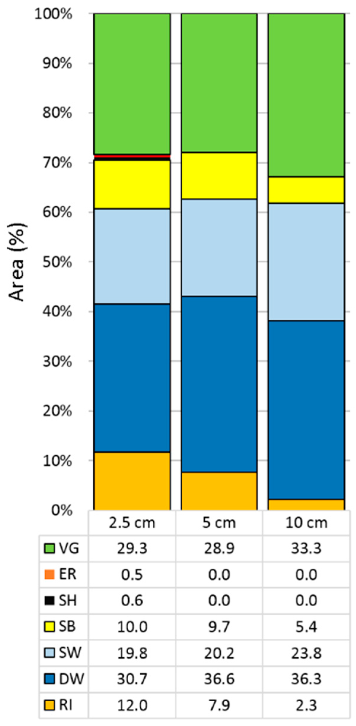
The per-pixel analysis shows that, based on a total of 67,446,624 pixels (2.5 cm × 2.5 cm), the dominant classes within the reach are deep water and vegetation, followed closely by shallow water (
Figure 5). The proportion of area allocated to the riffle and side bar feature classes decreases as the resolution coarsens, with erosion and shadow being present only on the 2.5 cm resolution imagery. By contrast, the proportion allocated to shallow and deep water is larger at coarser resolutions, with incremental changes from 5 cm to 10 cm resolutions.
The outputs for the Cochran test (
Table 6) show that the mismatch in feature allocation at per-pixel level between the 2.5 cm resolution and the coarser resolutions is statistically significant (
p < 0.001) for all features. Excluding erosion and shadows, riffle is the feature class with the largest percentage of pixels mismatched, followed by side bar and shallow water (
Figure 4 and
Figure 5).
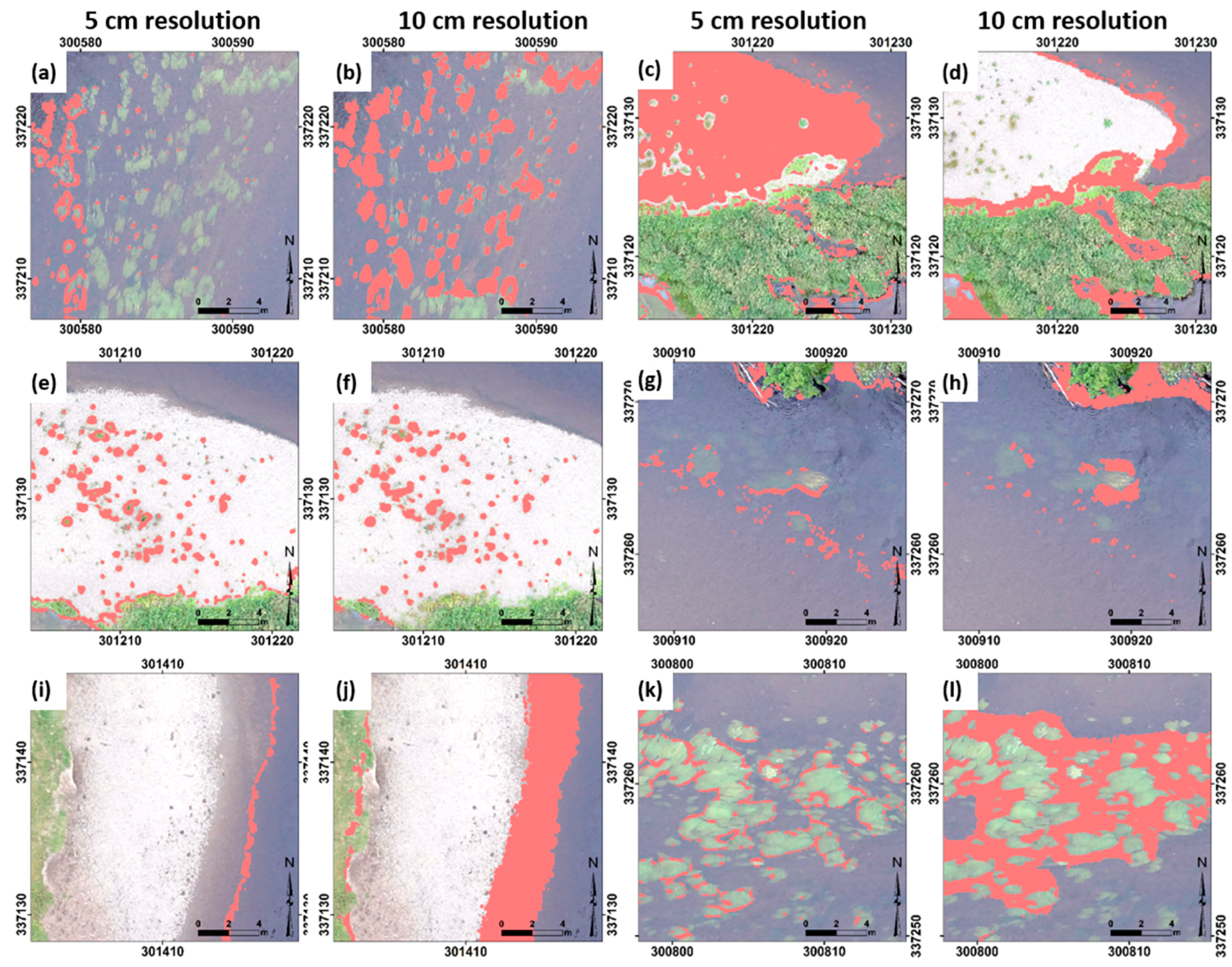
Figure 6 shows where the per-pixel misclassification occurs. For vegetation, mismatching pixels are primarily observed over submerged vegetation or side bars. For side bar, mismatch occurs on the edges, with coarser resolutions being unable to accurately detect the limit of the feature or the feature in itself. For deep and shallow water, mismatch occurs in areas of transition between the two features or around banks and submerged vegetation, whereas in the specific case of riffles, misclassification occurs for the overall class in general.
4. Discussion
This study focused on three core objectives: (i) to quantify the performance of an ANN based framework for hydromorphological feature identification for a set of aerial imagery resolutions; (ii) to identify the optimal aerial resolution required for robust automated hydromorphological feature identification; and (iii) to assess the implication of results obtained from (i) and (ii) in a regulatory context.
Where the first two objectives are concerned, the aerial imagery resolution plays a key role in the number, accuracy and variety of features automatically identified with LAIC. The coarser the resolution, the lower the number of features mapped within a river reach and the larger the bias in the detection of their extent. This is clearly visible for the specific case of riffle, side bar and erosion features, which are absent or barely identifiable from resolutions coarser than 5 cm. The patterns generated by the unbroken and broken standing waves that characterise riffles are not identifiable from the coarser (10 cm) imagery and get confused with classes that are more general, such as shallow and deep water. Similarly, at coarser resolutions submerged vegetation as well as vegetation on side bars fail to be identified properly. The power to delineate and identify side bars also decreases when imagery of resolution coarser than 2.5 cm is used. In addition, the distinction between deep and shallow waters cannot be drawn and misclassification occurs near submerged vegetation and banks.
The per-pixel analysis shows that these differences are statistically significant for all features and resolutions. However, these statistically significant differences need to be interpreted from a hydro-ecological perspective since these can be key to the structuring of freshwater biotic communities [
6]. The failure to identify both riffles and submerged vegetation will have an impact on the overall assessment of the reach, not just from the hydromorphological point of view but also from a biological context, as these features define key habitats for freshwater ecosystem species. For example, several authors [
38,
39,
40,
41] have identified riffles where gravels are present as the preferred areas for salmonid species to spawn. Underestimation of the area suitable for spawning will occur whenever the combination riffle–shallow water is not adequately identified. Likewise, flow type diversification over space and time, pool–riffle sequences and morphological impairment directly relate to habitat-scale interpretation and invertebrate community [
7]. Failure to characterise riffles, deep and shallow waters will directly impact upon the assessment of the reach suitability for macroinvertabrates. Failure to estimate submerged and emergent vegetation abundance and coverage will directly impact on the estimates of the area available for key habitats such as refuge, feeding, spawning and nesting [
42].
Gurnell [
43] reviews recent research on the geomorphological influence of vegetation within fluvial systems. The emergent biomass modifies the flow field and retains sediment, whereas the submerged biomass affects the hydraulics and mechanical properties of the substrate. A bias characterisation of the vegetation present within a reach will result for example, in biased estimates of erosion susceptibility. The uncertainty generated by the lack of power identifying side bars will also add to the bias in the estimation of risk from erosion and increase the difficulty in the detection of erosion and deposition patterns. This in turn will impair the accurate estimation of temporal changes in river reach boundaries, width and bank location (e.g., [
44,
45]).
The automated classification of hydromorphological features works in a similar way as visual identification would do. The algorithms LAIC applies are based on the RGB properties observed in the imagery, similar to what a field surveyor would detect when generating maps of homogeneous features in the field or from the aerial imagery. In [
19], the LAIC classification was shown to be more accurate than visual feature identification. For example, LAIC was able to identify the water between tree branches along the river bank. Assuming the classification from the 2.5 cm resolution to be a true representation of the hydromorphological variability within the reach, it can be inferred that visual identification of features from imagery at coarse resolution will incur the same errors as those identified here with LAIC.
Whether an optimal resolution for hydromorphological characterisation can be proposed is difficult to ascertain since there is a strong trade-off between accuracy and area surveyed. If accuracy is of concern, then a fine resolution of 2.5 cm is required. Alternatively, if wide area coverage is of interest, coarser resolutions than 10 cm would be preferred. For regional or even national assessment of river hydromorphology, automated identification of river features from high resolution UAV aerial imagery could be integrated in existing GIS frameworks (e.g., [
46,
47,
48,
49]) that operate with coarser resolutions and alternative remote sensing data supports (e.g., satellite imagery). Gurnell et al. [
50] recognises the benefits of using high resolution UAV aerial imagery to open further possibilities for improving the ability of frameworks to generate highly informative outputs in shorter time intervals and at smaller financial costs than at present. These enhancements will enable validation and calibration of current methods, frameworks and models for hydromorphological characterisation and intercalibration. The adoption of high resolution aerial imagery for hydromorphological characterisation at national level will significantly increase the demand for UAV based data capture. In UK, this can be provisioned through the deployment of platforms at the local level via the already existing network of 1557 CAA qualified providers [
51] if detailed guidelines on data requirements are specified.
Another factor to take into account when selecting the UAV imagery resolution is the coregistration error associated to the geomatic products generated. These are considerable for 10 cm resolution orthoimages, with 19 cm error in x, 83 cm in y, 55 cm in z and up to 3 m combined error in x, y and z. If UAV data collection is undertaken on a regular basis to assess temporal changes in hydromorphological characteristics, the errors identified may prevent the accurate spatial collocation of river features and restrict the accuracy of the change metric estimated (e.g., river width, volume of sediments deposited). In addition, results indicated that the disagreement in feature classification, when using the 2 m × 2 m grid as ground truth, is primarily dominated by spatial disagreement (i.e., location of features) rather than quantity disagreement (i.e., proportion of area allocated to each feature) and increases as the resolution coarsens. The combination of both coregistration error and spatial disagreement highlights the ineffectiveness of coarse resolutions for accurate hydromorphological characterisation.
Where the third objective is concerned, the study clearly demonstrates that commercially available aerial imagery at resolutions coarser than 10 cm does not provide sufficient robustness for unbiased hydromorphological assessment. Use of these supports result in biased feature coverage estimates, incorrect heterogeneity metric estimates and uncertain in-channel feature characterisation. This is consistent with results obtained by Carboneau [
29] who found that aerial imagery at coarse resolution (10 cm) was unsuitable to estimate grain size reliably. The selection of a given support will depend upon the objective the assessment needs to fulfil and will be conditioned by the trade-off between data acquisition costs and assessment uncertainty.
Outcomes from this research raise concerns about current practice in hydromorphological assessment and the need for the generation of uncertainty estimates. To the author’s knowledge, little work has been carried out to assess the uncertainty that the use of specific supports add to the overall hydromorphological characterisation. This is particularly relevant for policy and regulatory implementation as well as restoration management. Within the context of the Water Framework Directive, the intercalibration process aims to obtain comparability of ecological status boundaries and national assessment methods across Europe [
52]. The intercalibration has focused on the harmonisation of the position of high/good and good/moderate boundaries for specific ecological quality parameters but has not looked at the precision of these estimates [
4,
53] which, as shown in this paper, will change according to the data support (i.e., resolution) used. This work demonstrates that for consistent and unbiased aerial imagery based hydromorphological assessment across EU Member States it is paramount to standardise the support used to obtain comparable ecological quality parameter estimates. Failure to do so could imply consequences in the management practice of water authorities (e.g., penalty payment) in terms of measures and efforts undertaken to accomplish the WFD [
10]. In addition, results from the intercalibration process [
4] identify as inadequate the spatial scale (few 100 m) of physical-habitat based hydromorphological methods and highlights the need for remote sensing based methods that enable detailed site-specific data collection to expand their application to a large number of water bodies. This study demonstrates that both shortcomings can be easily overcome through the application of the framework presented here.


