1. Introduction
The use of LiDAR (Light Detection and Ranging) data for forestry applications has advanced in many ways in recent years, described, for example, by [
1] with a series of methodologies along with case studies. In particular, research into obtaining tree species/genera information from LiDAR has been increasing and classification results have been reported by several researchers including [
2,
3,
4,
5,
6,
7,
8,
9,
10,
11,
12,
13] and continues to gain greater attention. However, there are two common challenges in using LiDAR to classify tree species/genera that have received little attention in the literature. The first challenge is the existence of tree genera classes in the forest that have not been field validated. In supervised classification, this is a problem which arises when the validation data have more classes than the training data and it is a fundamental problem for sampling a subset of a population during training. In this case, normally an “unknown class” will be assigned to the extra class as has been described in [
14,
15]. The second challenge is the acquisition of inconsistent data from specific 3D tree objects, due to occlusion of tree parts due to varying LiDAR scan angles and canopy architecture. Moreover, when trees grow closely together, branches (and therefore LiDAR points) are often co-mingled among multiple trees and their membership to a specific tree canopy cannot be determined. Single trees having multiple tops or leaders can also be confused quite easily as being multiple trees, and variability in growing environments or tree age can lead trees of a common species to appear vastly different in LiDAR point clouds. This results in a large variation in training and validation samples, in terms of appearance and quality. This paper addresses these two issues by proposing a workflow that takes advantage of the variability observed within a common genera.
The use of ensemble methods is proposed to address this problem. Ensemble classification is the training of multiple classifiers to solve a common labeling problem by different communities. This classification strategy is also called committee-based learning, multiple classifier systems, or a mixture of experts [
16,
17,
18]. The criterion of a good ensemble system is that it should provide an increase in classification accuracy. There are numerous ways of combining classifiers as suggested by previous studies [
19] with a wide variety of applications contributed from text categorization [
20] and hand-written word recognition [
21]. In particular, a few examples of related studies in remote sensing include [
17,
22,
23,
24].
There are three popular techniques for reducing a multi-class problem into a series of binary classification problems [
25], namely: “one-versus-one” (OVO) [
26], “one-versus-all” (OVA) [
27], and Error Correcting Output Codes (ECOC). OVO consists of binary classifiers that differentiate between two classes (for example pine vs. maple), and therefore for a
k class problem,
(or “
k combination 2”, calculates the number of combinations needed to separate
k classes with only two outcomes for each classifier, namely “positive” and “negative”) classifiers are needed for ensemble implementation. On the other hand OVA consists of binary classifiers that discriminate between particular classes from the rest of the classes (for example, pine vs. non-pine), and therefore
k classifiers are needed to solve a
k-class problem. ECOC is a method where a code word is generated from a series of binary classifiers for each class label. For any validation sample, a code word from that sample will be generated, and compared to the code word generated from the training samples. The class with the minimum Hamming distance will be labeled [
28]. To compare the performance between OVO and OVA, studies such as [
25] show that although there is no significant difference found between OVA and OVO, both strategies outperform the original classifier. In another study, the authors of [
29] showed that OVA attains more accurate classification when comparing: (i) a concept-adapting very fast decision tree (CVFDT), a single multi-classifier; (ii) a weighted classifier ensemble (WCE), and streaming ensemble algorithm (SEA), both of which are ensembles of multi-class classifiers; and (iii) an ultrafast forest tree (UFFT), an OVO method. In [
30] it was shown that OVO outperformed OVA, in contrast to [
27] where it was suggested that OVA performed as well as OVO. These studies suggest that neither OVO, nor OVA, consistently outperform the other. Instead, these studies indicate that the decomposition of a multiclass problem into series of binary classification problems is an efficient approach that often outperforms the original multi-class classifier. In fact, OVO and OVA are popular methods for combining Support Vector Machine (SVM) classifiers [
30,
31,
32,
33].
As mentioned earlier, it is not always easy to obtain a completely isolated single tree; as a result, the “data quality” of segmented LiDAR trees is not uniform. Consequently, when training data are randomly selected from these segmented LiDAR trees, the problem of imbalanced training, with respect to data quality, arises. Normally, the problem of data distribution imbalance refers to the differences in the number of samples for each class [
34,
35], which is a common problem in real world data simply because some phenomena occur infrequently in nature. Classifiers generated from an imbalanced training sample will be specialized in classifying the majority classes, and therefore will bias the results towards the majority class. At the data level solution, there are three common techniques to overcome this problem: (1) oversampling the minority class; (2) under sampling the majority class; or (3) a combination of both methods [
34,
35,
36,
37,
38]. The goal of these strategies is to diversify the sampling distribution in terms of the number of samples per class and these studies show that the distribution of the training sample is important in affecting the classification accuracy.
Diversification is an important concept in ensemble learning; when the classifiers to be combined have substantial diversity, the predictive power tends to be higher [
39]. During the construction of the Random Forests classifier, the classifier already incorporates the concept of diversification in the following ways. According to [
40], Random Forests diversify the number of training samples by bootstrap aggregating (bagging) in two ways. First, the same number of samples are drawn from the minority and majority class, balancing the minority/majority sample. Second, a heavier penalty is placed on misclassifying the minority class by giving it a higher weight, and the final label takes the majority voting of the individual classification trees. Also, during the construction of an individual classification tree, a subset of features is selected for defining the splitting node. The subset of features is drawn randomly and this randomization promotes diversification in classification. The authors of [
41] further increased the diversity of Random Forests by splitting the training samples into smaller subspaces, and showed improved classification accuracy in their medical datasets over regular Random Forests classification. However, improving the performance of supervised learning through balancing the per-class distribution of training samples can be achieved only if the quality of individual samples exhibits relatively similar condition across and within classes. As discussed earlier, the segmentation quality of LiDAR tree samples is irregular, and its regularization is a non-trivial task, especially using 3D LiDAR point clouds captured in forest environments.
There are two goals for this paper: First, to address and quantify the quality of variability observed in the data that have been field validated. From those results, the relationship between the diversity present in the training samples are examined in relation to the ultimate classification accuracy. Second, training data are selected that contain the most diversity, and classification is performed using a series of binary classifiers with a scheme that has been designed to generate an “unknown” class. This will address the problem of having more classes in the validation data than the training data.
2. Study Area and Data Acquisition
The LiDAR data were collected on 7 August 2009, over field study sites located about 75 km east of Sault Ste. Marie, Ontario, Canada. A Riegl LMS-Q560 scanner on multiple flight passes was flown at altitudes between 122 and 250 m above ground level; the combined pulse density of the dataset is about 40 pulses per m
2. Since each pulse generates up to five returns, the point density can be as high as 200 points per m
2. The data were acquired at a lower altitude for the power-line corridor site to obtain a higher point density data for the purpose of power line risk management, whereas the other forested sites were acquired at a higher altitude. Field surveys were conducted in the summers of 2009 and 2011 at eight field sites (
Table 1), selected to capture the diversity of environmental conditions, and are named:
Poplar1,
Poplar2,
Maple1,
Maple2,
Maple3,
Pine1,
Pine2, and
Corridor. The poplar sites (
Poplar1 and
Poplar2) contain mostly poplar trees, which are located in the northern part of the study area.
Maple1,
Maple2, and
Maple3 are dominated by maple, and share very similar characteristics. All the maple-dominated sites have a closed canopy, and are growing with other deciduous species such as birch and oak; the understory growth is vigorous.
The Corridor site is the most complex site, and was selected because it includes trees that are difficult to identify from LiDAR data. The trees in the corridor sites are growing very close together, such that individual crown isolation from the LiDAR data for this site is difficult and often the LiDAR derived tree crowns that were isolated into individual trees, contain points from neighboring trees. Furthermore, some LiDAR tree crowns collected from this site contain partial occlusion by shadows, and also the site is characterized by vigorous understory growth. The growing conditions between the two sides of the transmission corridor are also different due to the differences in topography, resulting in differences in sunlight penetration to the vegetated area, as well as in the abundance of understory growth. One side of the site has abundant understory growth whereas the other side has very little.
The pine-dominated sites (
Pine1 and
Pine2) were selected to represent an open canopy area. Pine
1 is dominated by red and white pine and Pine
2 is dominated by white pine stands. Of the 186 trees sampled, 160 of them belong to
Pinus (pine),
Populus (poplar) or
Acer (maple), which are the three main genera (class labels) of classification for this paper. The rest of the trees (26 trees) will be treated as other category, and will be classified as “unknown”, which contain 11
Betula (birch), 3
Quercus (oak), 10
Picea (spruce), 2
Larix (larch) (
Table 1). Within the tree genera collected in the field sites, the identified species are white birch (
Betula papyrifera Marsh.), maple (
Acer saccharum Marsh.), red oak (
Quercus rubra L.), jack pine (
Pinus banksiana Lamb.), poplar (
Populus temuloides), white pine (
Pinus strobus L.), white spruce (
Picea glauca (Moench) Voss), and larch (
Larix laricina).
3. Methods
3.1. Overview of the Methodology
In ensemble learning, there are two types of models. The first is the parallel ensemble model where base learners are used to make decisions in parallel (e.g., bagging methods). The second is the sequential ensemble model where base learners are used to make decisions sequentially (e.g., boosting methods) [
18]. One of the most important objectives for combining classifiers is to reduce the overall error, that is, to increase the overall classification accuracy as compared to a single classifier [
24,
42,
43,
44,
45]. In parallel models, [
18] showed mathematically that errors reduce exponentially to ensemble size
T by the Hoeffding inequality using the following example: Let
hi be the base classifier (binary) {+1, −1} with error
such that
where
f(x) is the field validated data, and by combining
T classifiers, one can form a regular ensemble classifier
H(x):
where
.
Assume that if the final decision is made by a majority voting scheme,
H(x) will misclassify if at least half of the base classifiers make an error. Therefore, the generalization error can be written as:
This shows that the generalization error reduces exponentially as T becomes larger, such that as .
In sequential models, the overall errors are reduced in a residual decreasing manner. An efficient sequential model has base classifiers ordered in a way that the subsequent base classifier is able to correct the mistake of a prior base classifier. Also, base classifiers will have to be sufficiently diverse such that the same mistake will not be made in the succeeding level.
For this paper, classification is performed with two models, but because the parallel model shows better classification accuracy, our discussions will be restricted to the parallel model. Since one of the goals for this paper is to design a classification scheme that is capable of classifying the negative samples (the non-pine, non-poplar, and non-maple), the OVA decomposition is more suitable for this task. We use the OVA decomposition within a parallel model for classifying pine, poplar, maple, and “unknown” with Random Forests as our base classifiers. The process comprises three main components: (1) selection of training and validation samples; (2) using Random Forests as base classifiers; and (3) running the parallel ensemble model. Random Forest classification is discussed first although it is the second step in the overall methodology, primarily because the other components rely on an understanding of Random Forests classification.
3.2. Random Forests Classification
In this paper, each “LiDAR tree” refers to an individual, isolated tree that contains LiDAR points that are segmented from the LiDAR point cloud scene whereas classification tree refers to the decision tree constructed by the Random Forests method. As alluded to earlier, increased diversity is important for improving classification performance; Random Forests has already applied this concept by balancing the number of training samples per class, and had included randomization in selecting training samples, and features for splitting node definitions. We will further increase diversity by having as much variety in terms of data quality in training samples as possible. Random Forests is being used in two different areas in this paper. The first is for quantifying the quality of each LiDAR tree; this information is then used for the final selection of training data. An experiment is also performed to show the change in classification accuracy due to the increase in diversity included in the training sample. Since this part of the analysis is for selecting training samples, where training samples contain no “unknown” class (as training samples had been field validated), the Random Forests classifier is used as a multi-class classifier. The second way that Random Forests classifier is used is for constructing the binary base classifiers where classification will be performed on the validation data. There are three base classifiers: hp (classifier that will produce class labels of pine (p) and non-pine (p’)); ho (classifier that will produce class labels of poplar (o) and non-poplar (o’)); and hm (classifier that will produce class labels of maple (m) and non-maple (m’)). In this paper, we refer to Random Forests that is being treated as a multi-class classifier as Regular Random Forests (R-RF) in order to differentiate it from Ensemble Random Forests (E-RF).
The Random Forests algorithm itself is an ensemble classifier, where the final classification labels are obtained by combining multiple classification trees for categorical data, or regression trees for continuous data trained from a subset of the data [
46,
47]. Random Forests uses approximately 63% of the data for training (in-bag data) and therefore uses approximately 37% of the data (out-of-bag data) for validation. The value 37% comes from the approximation of the value
where a number of observations
N is drawn with replacement and therefore
of data are being omitted from the draw and therefore it is called “out-of-bag” (OOB). The main input variables for Random Forests relevant for this paper are: (1) training sample labeled with known genera, and a description of the geometric classification features; the detail for deriving these features can be found in [
48]; (2) the number of feature variables randomly sampled at each split (
Mtry = 2); (3) the number of trees generated within each iteration (
Ntree = 1000); and (4) minimum size of terminal node (
Knode = 1). These values were set according to the suggestion from [
49] where
Ntree is a large number;
Mtry ≈ square root of the number of features and nodesize = 1 is the default for classification trees. Random Forests produce the following output relevant for this paper: (1) a classification scheme generated using in-bag training data; (2) the mis-classification rate as a percentage using OOB data; and (3) average vote calculated for each class in each LiDAR tree, where the final prediction of the OOB data are made by the maximum average vote. The classification algorithm was implemented within the
randomForest package for R [
50].
3.3. Goal 1: Maximizing Quality Diversity in the Training Data
In this part of the experiment, the quality of each LiDAR tree is quantified as has been validated in the field as belonging to pine, poplar, and maple. One can only quantify LiDAR trees belonging to these genera because a subset of these trees eventually became our training data, where our validation data will contain the “unknown” class. A sensitivity analysis is also performed on how data quality affects classification accuracy, since it was assumed that a larger range of quality in training sample would yield higher classification rate. With the lack of field validated data, it was decided to include all the field validated LiDAR trees for running the experiment excluding the “unknown” instances for testing diversity against classification accuracy. As mentioned before, Random Forests randomly select approximately 37% of the data (OOB data) as validation. A class prediction is made for each LiDAR tree that is selected as OOB data, from which an OOB error is calculated. One of our research goals is to propose a quality index measuring a diversity of training data quality used for learning Random Forests. Through maximizing the diversity of training data quality, we aim to improve classification accuracy obtained by Random Forests classification.
Suppose that we have a training dataset,
T, which contains
k LiDAR trees, that is
T = {
ti|
t1,
t2, …,
tk}, where
k = 160 tree samples in our case. Given a set of
T,
OOB data are generated by randomly selecting
Ntree numbers of its subsamples,
OOB = {
OOBj|
OOB1,
OOB2, …,
OOBNtree}, each of which is used for producing a set of decision trees,
h = {
hj|
h1,
h2, …,
hNtree}. Then, we can measure
NCi and
NDi for any given
ti by introducing two indicator functions
IC(ti) and
ID(ti) as follows:
where
NCi indicates the number of times a LiDAR tree (
ti) is predicted correctly, while
NDi represents the number of times a LiDAR tree (
ti) is selected as OOB data;
hj is the base classifier, and
f(ti) is the field validated data. Next, we compute a data quality
Qi, which can be described as:
Qi from Equation (6) is a measurement being made of the ith LiDAR tree sample, and is normalized by the denominator NDi. If Qi is small, it means that the particular LiDAR tree cannot be correctly predicted easily, and vice versa. Qi has a minimum value of 0 where the particular tree can never be classified correctly and a maximum value of 1 where the particular tree can always be classified correctly. This ratio will represent data quality for the rest of the paper. The data quality measure described in Equation (6) is calculated over the entire training set T to produce {Qi}.
To obtain classification accuracy of validation data, the OOB error provided by Random Forests classifier was not used. Instead, 25% of the total data were partitioned for training and 75% of the data for testing (and to obtain the classification accuracy). A previous study [
48] shows that a 25%:75% ratio for training and validation is optimal for this dataset and therefore this same ratio will be used to perform the following experiments.
Next, we plot a frequency distribution over {
Qi} computed by Equation (6). Then, we had quantized {
Qi} into
a bins (where
a = 10), from the entire training set
T. Subsequently, from this distribution, we select 25% of the data (
N) optimally with maximized diversity where each bin contains approximately
LiDAR tree samples. We can only approximate
for two reasons: (1)
, but the number of samples in each bin is an integer; (2) in the case where the number of samples per bin is less than
, the sample gets allotted to another bin such that
remains 25% of the number of total samples. We than characterize the distribution of data quality by calculating our diversification index,
DI, using Equation (7):
where
a = number of bins,
N = number of training data,
Ni = number of training data in the
ith bin, such that
.
When the distribution of the dataset across bins is uniform, each bin contains () samples, DI = 1, indicating the most diversified distribution of Qi contained in the training data. When selected N is contained in a single bin, DI = 0, indicating the least diversity in the distribution of Qi. To test the relationship between DI, and classification accuracy, we restrict our range of Qi ten times, each time the range begins from 0.0 and ends at a threshold increasing from 0.1 through to 1.0 in 0.1 unit increments; within each of these ranges we calculate: (1) DI; (2) the classification accuracy for R-RF without “unknown” samples in the validation data; (3) classification accuracy for R-RF with “unknown” samples in the validation data; (4) classification accuracy for E-RF to be discussed in the next section, without “unknown” samples in the validation data; and (5) classification accuracy for E-RF to be discussed in the next section, with “unknown” samples in the validation data.
3.4. Goal 2: Ensemble Random Forests (E-RF)
The optimized set of training samples (47 LiDAR trees, 10 bins) from the previous section are used for training the base classifiers, the remaining 139 trees are used as validation data. The selected training data are used for training the three base classifiers, , , and with maximized diversity, allowing the base classifiers to learn as much variability as possible.
The parallel model is summarized in
Table 2, where
,
, and
are the base classifiers. In the model, the base classifier simultaneously classifies pine (non-pine), poplar (non-poplar), and maple (non-maple) at the same time. In cases where there are no conflicts in decisions made among the base classifiers (i.e., Cases 1, 2, 3, 8), the final decision is made by the classifier voted for by a positive case (Cases 1, 2, and 3). Where all three classifiers vote negatively (Case 8), the tree will be labeled as “unknown”. In the cases where classifiers are conflicted (Cases 4–7), the final decision is made by the classifier that has the majority positive vote. A majority vote is calculated by Random Forests over
T base classifiers described in Equation (8) [
50]. The classification accuracy of this model, ensemble Random Forests (E-RF) is compared with regular Random Forests (R-RF).
where
is the features selected for classification;
is the binary indicator variable for voting the
L instances with given
X;
y is the predicted class label such that
y ∈
L, and
y* is the final prediction for a particular base classifier.
5. Discussion
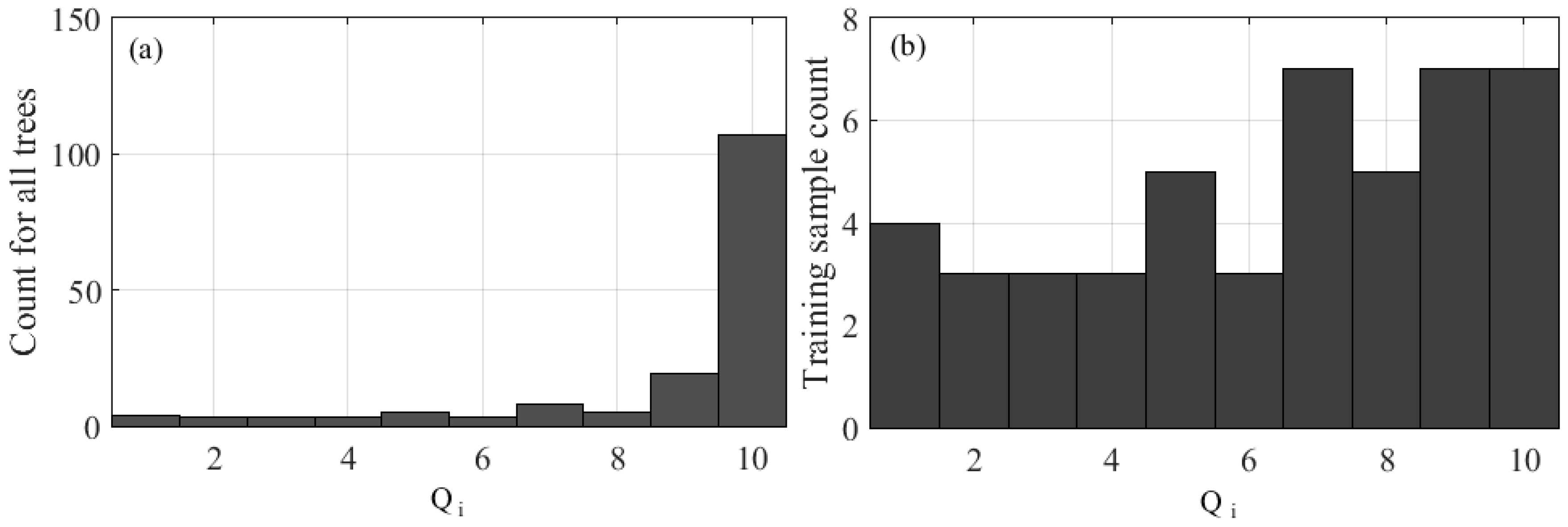
The majority of the data collected for this research have similar properties; by randomly selecting the training data we ensure that the training data will have a similar statistical distribution as does the population. Given that the majority of the training data is similar, any validation data that deviates from the training data will be misclassified. To solve this problem, the quality of collected samples is quantified by computing
Qi, and the frequency distribution examined (
Figure 1a) so that a diversified training sample is obtained (
Figure 1b). When training samples are selected randomly from the distribution as shown in
Figure 1a, there is a higher chance of having empty bins in the training data due to lower frequencies in the lower
Qi bins, resulting in lower diversity in the training data. As a result, when base classifiers are trained based on randomly selected samples (with lower diversity), more emphasis will be placed on the LiDAR trees that have a high
Qi. We propose using a distribution such as in
Figure 1b for training sample selection in order to maximize diversity where training samples contain trees that have both low, and high
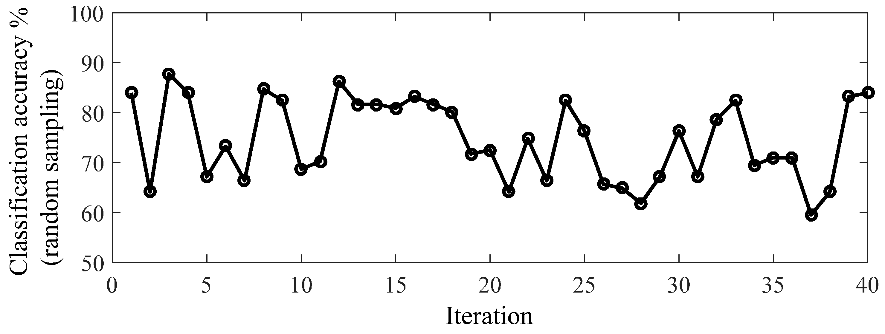
Qi, resulting in improved classification accuracy with such a selection. The classification accuracy assessment is compared through two comparative experiments: in the first experiment the classification results are compared from E-RF random sampling versus E-RF with diversified training samples (
Figure 1b) by comparing results shown in
Table 3 and
Table 4; in the second experiment, the classification results are compared between R-RF and E-RF, both using the diversified training samples by comparing results shown in
Table 4 and
Table 5.
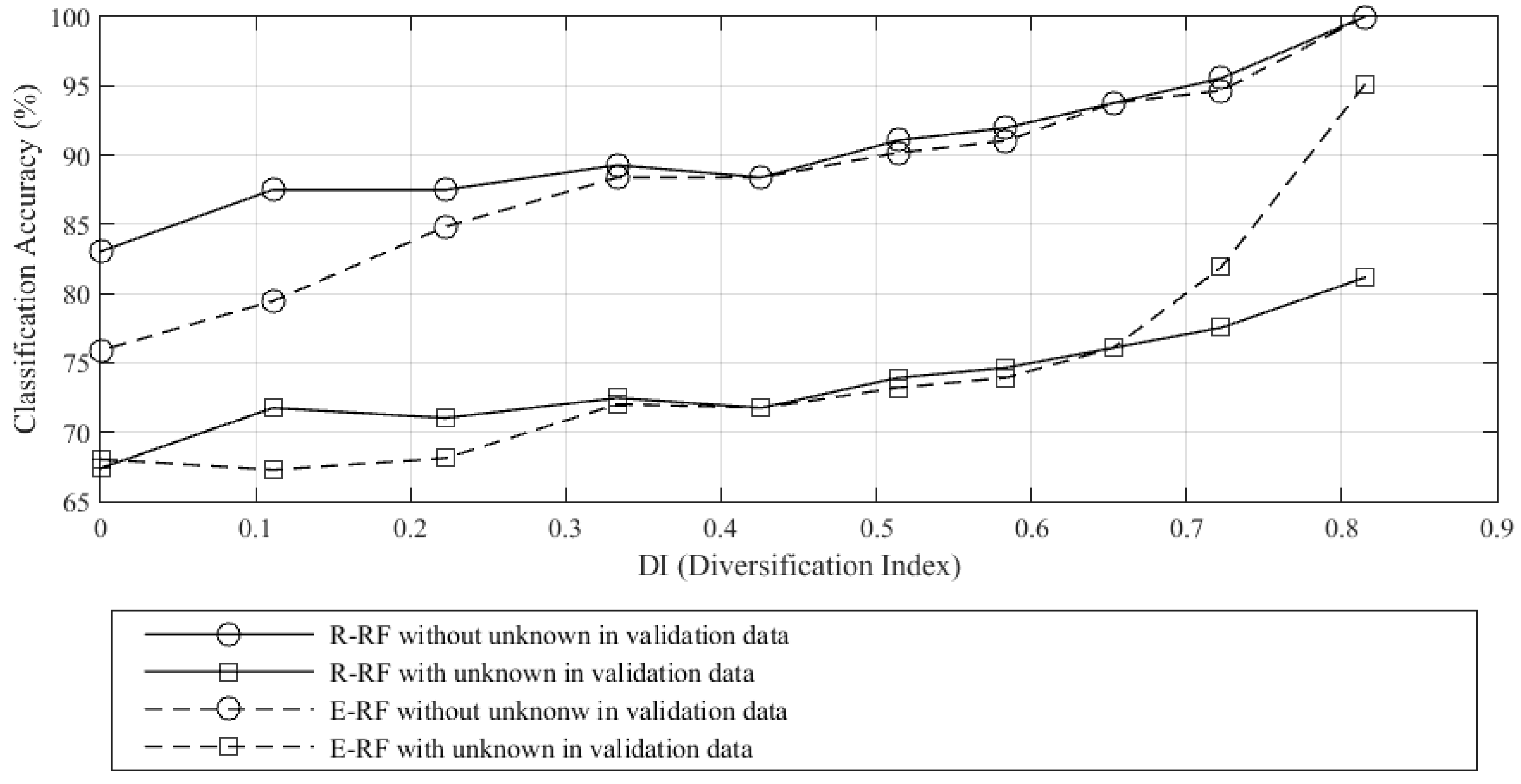
In
Figure 3, the smallest value of
DI is zero when all training samples are drawn from one class; this is the least diversified example. Alternatively, the largest value,
DI = 0.82 is the most diversified training sample attainable (
Figure 1b), where the samples were not able to distribute uniformly across all calculated
Qi bins. In theory,
DI = 1.0 if all the samples are distributed uniformly across all bins. When
DI increases, the classification accuracies also increase (both with and without unknown samples in the validation data). This shows that diversity in the training data improves classification accuracy, regardless of the choice of algorithm or the presence of an “unknown” class in the validation set. This result indicates that taking
DI into consideration during training is advisable. We believe that the variations in classification accuracy observed in
Figure 4 are attributed to differences arising from the selection of training samples. We further observe that when unknown samples are included in the validation data, E-RF is outperformed by R-RF by 4.3% and 13.9% when
DI = 0.72 and 0.82 respectively. This refers to training data which include values of
Qi from 0.0–0.2 and 0.0–0.1, respectively. These results imply the importance of including low
Qi samples in the training data. Given that E-RF outperformed R-RF implies that the higher
DI included in the training data are more effective than the R-RF and in the future, E-RF should be a preferred choice for classification, especially with maximized
DI. Conversely, if
DI is small, R-RF and E-RF exhibit similar performance with the presence of unknown samples in the validation set. Further, R-RF outperformed E-RF in the case where no unknown class is present in the data set and when
DI is small (<0.33). E-RF shows a lower classification accuracy compared to R-RF by 8.0% and 7.1% when
DI = 0 and 0.11, respectively, and when validation data are absent; in these cases E-RF should be avoided. However, this is normally not a real life situation where the validation data contain only classes obtained from the training data. Furthermore, it is hard to guarantee that the field-validated data will contain all tree species in the forest plot given the complexity of the natural environment.
Computed Shannon entropy for the Qi ranges and the plot of classification accuracies over different entropy values present corresponding results. However, since DI values are bounded between 0 and 1, their interpretation is easier and we propose the use of DI over entropy.
By comparing
Table 3 and
Table 4, the commission and omission errors were reduced to 60% and 53% respectively for the “unknown” class when the training sample is diversified. This is because the “unknown” classes are labeled based on the classification accuracies of negative samples from the base classifiers. When the training samples have low diversity, it indicates that most of the training samples appear to be similar and therefore the distributions of the features related to the specific class are narrow. As a result, any validation data that deviate from the training data will be classified as negative (high omission error, 84% in
Table 3, reduced to 31% in
Table 4). Conversely, when the training samples contains high diversity, the distributions of values for the features that train the base classifiers are broader allowing a broader definition of a specific class, reducing the chance of classifying negative samples as positive (commission error of “unknown” class reduced from 60% to 0%).
Since the training sample contains only pine, poplar, and maple, by default, the class labels generated from Random Forests will be the three mentioned classes. However, in order to be able to compare with ensemble methods, an additional condition is included so that “unknown” classes can be identified with Random Forests alone. As mentioned, for each validation sample in Random Forests, the final class label is assigned by the class with the majority vote stated in Equation (8). The additional condition is that if the majority vote calculated for the particular tree is less than 67%, it should be classified as “unknown” instead of one of the three classes. The additional condition ensures that the “unknown” class is assigned when the majority vote calculated for the particular tree is <67%. This threshold represents at least a two-thirds vote among the three classes in order to be valid.
Table 5 shows the confusion matrix obtained from Random Forests using diversified samples, where values are averaged by running the ensemble 20 times. Comparison of
Table 5 with
Table 4 shows that E-RF classification yields an overall accuracy of 93.8% whereas R-RF yields an overall accuracy of 88.4%. The omission error for R-RF is less than E-RF but the commission error for classifying poplar for R-RF is higher. With E-RF, the omission error for pine, poplar, and maple is also lower.
There are several reasons proposed for this improvement over the traditional multi-class classification: (1) E-RF are able to generate an “unknown” class without a pre-defined threshold; (2) the method does not require the presence of an “unknown” class in the training data; (3) the implementation of binary classification is simple, so that in the future, if another class label is being collected in the field, an additional binary classifier can be built but all the previous training results can be re-used without any changes; and (4) the method of combination can be altered and additional rules can be implemented to improve the aggregation of information such as in
Table 3. The methodology and discussion in this paper applies beyond the use of LiDAR for forest applications, as it is natural to obtain 3D data with varying quality. This study aids in making better choices related to the selection of training data, such that classification accuracy can also be boosted. Furthermore, the generation of an “unknown” class is practical for classification problems when there is a presence of classes in the testing data that were not included in the training data.
6. Conclusions
This study has two important conclusions, the first relates to the importance of diversifying the quality of training samples in order to improve classification accuracy. The quality of LiDAR tree samples can vary due to reasons such as shadow or occlusions from scanning angle effects, overlapping of adjacent trees or trees that appear to have multiple tree tops making tree crown isolation difficult. The problem of quality inconsistency, an inherent problem with 3D point cloud data, is an unavoidable problem that naturally occurs with all types of objects, not only trees. Intuitively we assume that a better sample quality should improve classification accuracy; our results show that high diversity in training samples helps with classifying negative instances and is especially useful in determining the “unknown” class.
This paper quantifies data quality, Qi, a term that is normally prone to subjective definition, and shows that by increasing diversity in the training data, classification accuracy can be improved. Diversity is a concept being applied to improve learning capacity in machine learning and we have included additional diversity beyond what the Random Forests algorithm already provides. By computing the DI we also quantify the amount of diversification in the dataset, the diversified Qi range (high DI) in the training data provide an improved accuracy. This paper was guided by the hypothesis that when the classifiers are trained with samples that contain as much variability as possible, there will be a better decision boundary between the positive and negative class labels. With a broader definition of each genus, results show that classification accuracy can be improved from 72.8% to 93.8%, both using E-RF, with the accuracy especially improved for the classification of negative labels. In the future, when we have increased number of samples, it would be possible to partition part of the data for the computation of Qi and select training samples from the computation. While we are unable to do this in this experiment, we have shown that the increased DI would provide improved classification accuracy and provides a basis for future research in this direction.
The second conclusion we can draw from this paper is the effectiveness of E-RF compared to R-RF. In E-RF, we have designed the base classifiers such that
k binary classification models are required for classifying
k classes. By combining these base classifiers instead of using R-RF as a multi-class classifier, a better accuracy result can be obtained (improved from 88.4% to 93.8%). Although the classification accuracy can be improved by implementing E-RF as suggested in comparing
Table 3 and
Table 4, nevertheless, the omission error for the “unknown” class is still the highest in
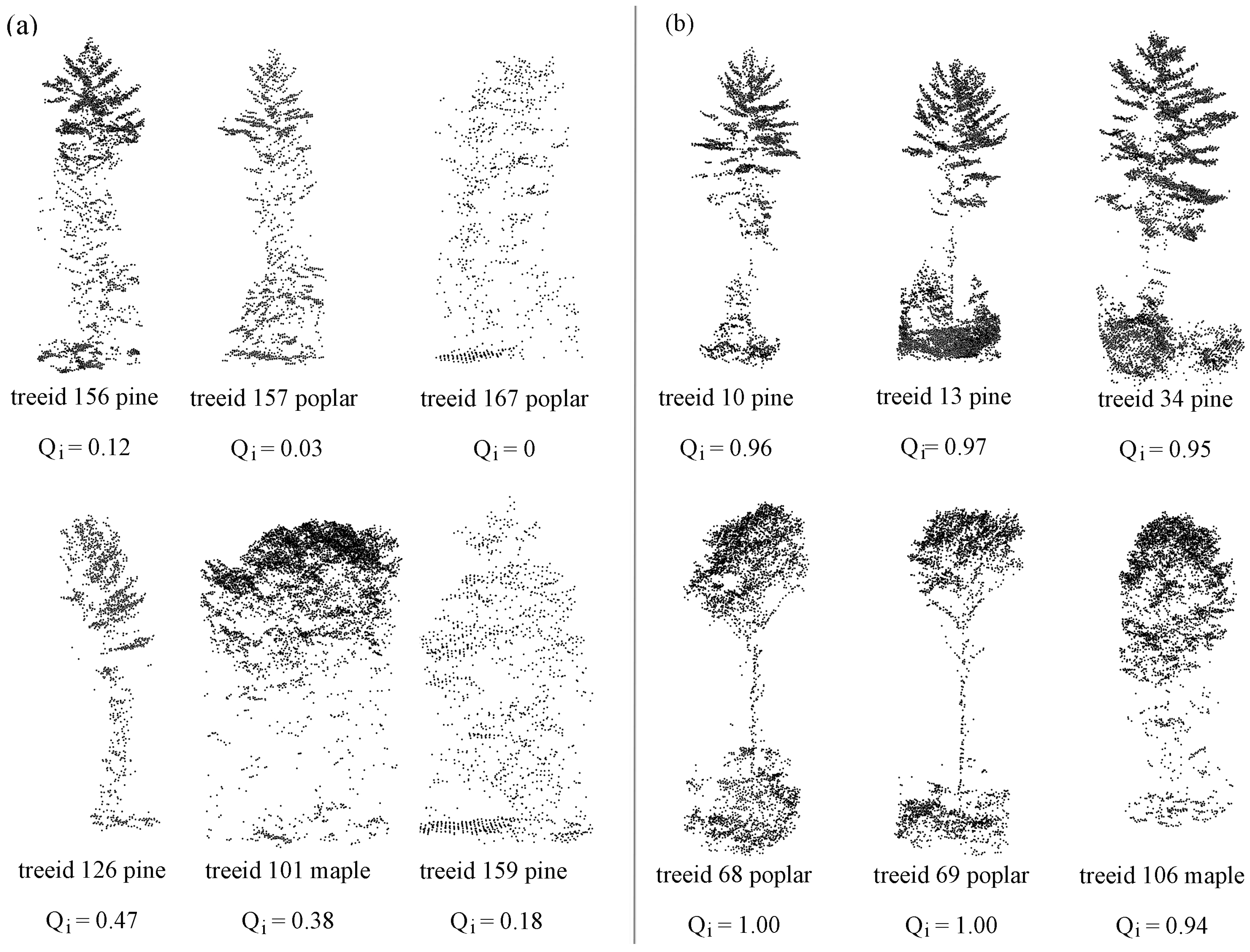
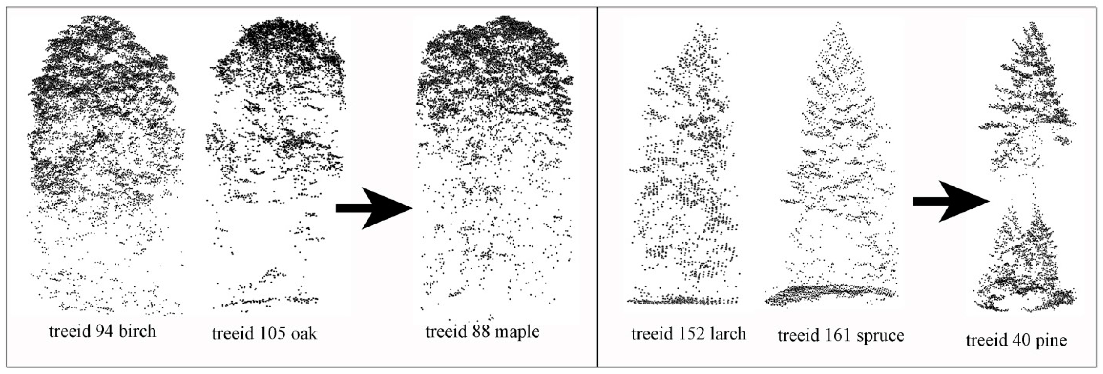
Table 4 when compared to other classes. This is because of the confusion of the similarities shared among genera. Examples are birch and oak trees are normally mistaken as maple trees; spruces and larch trees are normally mistaken as pine trees (
Figure 5). This problem can be resolved if new features for classification can be developed that are independent of geometry. This can increase the diversity in the classification features and enable building base classifiers that are capable of processing different types of information.
In this paper, we have proposed a method to quantify data quality by computing Qi. We have also examined the importance of having a diverse training data set in order to improve classification accuracy. Experimentation has shown that as DI increases, the classification accuracy increases. In our dataset, it is especially important to include the data with the lowest quality in the training data set in order to maximize classification accuracy; results show that classification accuracy improves from 72.8% (random sampling) to 93.8% (diversified sampling). To tackle the problem of having more classes in the validation data than training data, we proposed E-RF for the generation of an “unknown” class without implementing any threshold. Results show that E-RF (93.8%) outperformed R-RF (88.4%) when the DI was maximized.


