Multi-Probe Based Artificial DNA Encoding and Matching Classifier for Hyperspectral Remote Sensing Imagery

Abstract

In recent years, a novel matching classification strategy inspired by the artificial deoxyribonucleic acid (DNA) technology has been proposed for hyperspectral remote sensing imagery. Such a method can describe brightness and shape information of a spectrum by encoding the spectral curve into a DNA strand, providing a more comprehensive way for spectral similarity comparison. However, it suffers from two problems: data volume is amplified when all of the bands participate in the encoding procedure and full-band comparison degrades the importance of bands carrying key information. In this paper, a new multi-probe based artificial DNA encoding and matching (MADEM) method is proposed. In this method, spectral signatures are first transformed into DNA code words with a spectral feature encoding operation. After that, multiple probes for interesting classes are extracted to represent the specific fragments of DNA strands. During the course of spectral matching, the different probes are compared to obtain the similarity of different types of land covers. By computing the absolute vector distance (AVD) between different probes of an unclassified spectrum and the typical DNA code words from the database, the class property of each pixel is set as the minimum distance class. The main benefit of this strategy is that the risk of redundant bands can be deeply reduced and critical spectral discrepancies can be enlarged. Two hyperspectral image datasets were tested. Comparing with the other classification methods, the overall accuracy can be improved from 1.22% to 10.09% and 1.19% to 15.87%, respectively. Furthermore, the kappa coefficient can be improved from 2.05% to 15.29% and 1.35% to 19.59%, respectively. This demonstrated that the proposed algorithm outperformed other traditional classification methods.

1. Introduction

Hyperspectral imagery (HSI) has found many applications in various fields, such as military, agriculture, and mineralogy [1]. As one of the traditional hyperspectral analysis techniques, spectral matching classification is often used for signature discrimination, which concentrates on recognizing absorption band and shape of spectra [2]. Many spectral matching classification techniques have been proposed. They often depend on a scalar metric to estimate how close two spectra are. In general, they fall into two categories [3,4,5,6]. In the first category, traditional algorithms estimate the similarity of two spectra by comparing signature distance. For example, minimum Euclidean distance (MED) classification method divides the classes of land covers by calculating the Euclidean distance of spectral vectors. The smaller the distance value is, the more similar the land covers are. MED provides a similarity scale to estimate spectral brightness with high efficiency. Binary coding (BC) is another method comparing spectral signature brightness [7]. It calculates the mean value of spectral curve, and then the spectral curve is encoded to a sequence of zeroes and ones through mean-value-threshold. It may not provide a precise spectral matching result. Spectral distance based classification methods may lead the misclassification when image sunlight is insufficient or shadow exists [8,9]. In the second category, spectra are regarded as multidimensional vectors. The similarity of two spectra is estimated by comparing shapes. For example, spectral angle mapper (SAM) method calculates the generalized angle of two vectors. The smaller the angle is, the more similar the spectrums are [10,11]. Spectral shape based matching methods can avoid the partial noises, so a high accuracy of spectral matching result can be acquired. However, it is worth noting that some important details may be smoothed in these kinds of methods [12]. In addition, there are some other encoding works with successful performance are proposed for image processing. Spatial pyramid matching (SPM) divides image into blocks in different scales, then the histograms of local features in each block represent the image [13]. This approach achieved impressive performance of image classification. SCSPM incorporates sparse code (SC) into the framework of SPM. This variant of SPM achieves a higher recognition rate than traditional SPM [14]. However, it consumes more time for encoding the local descriptors. Low rank representation (Lrr) based spatial pyramid matching (SPM) method encodes the descriptors under the framework of SPM and calculates the representation in the matrix space directly [15,16]. It improves the robustness of the variants of SPM. LrrSPM achieves a better efficiency than the variants of SPM.

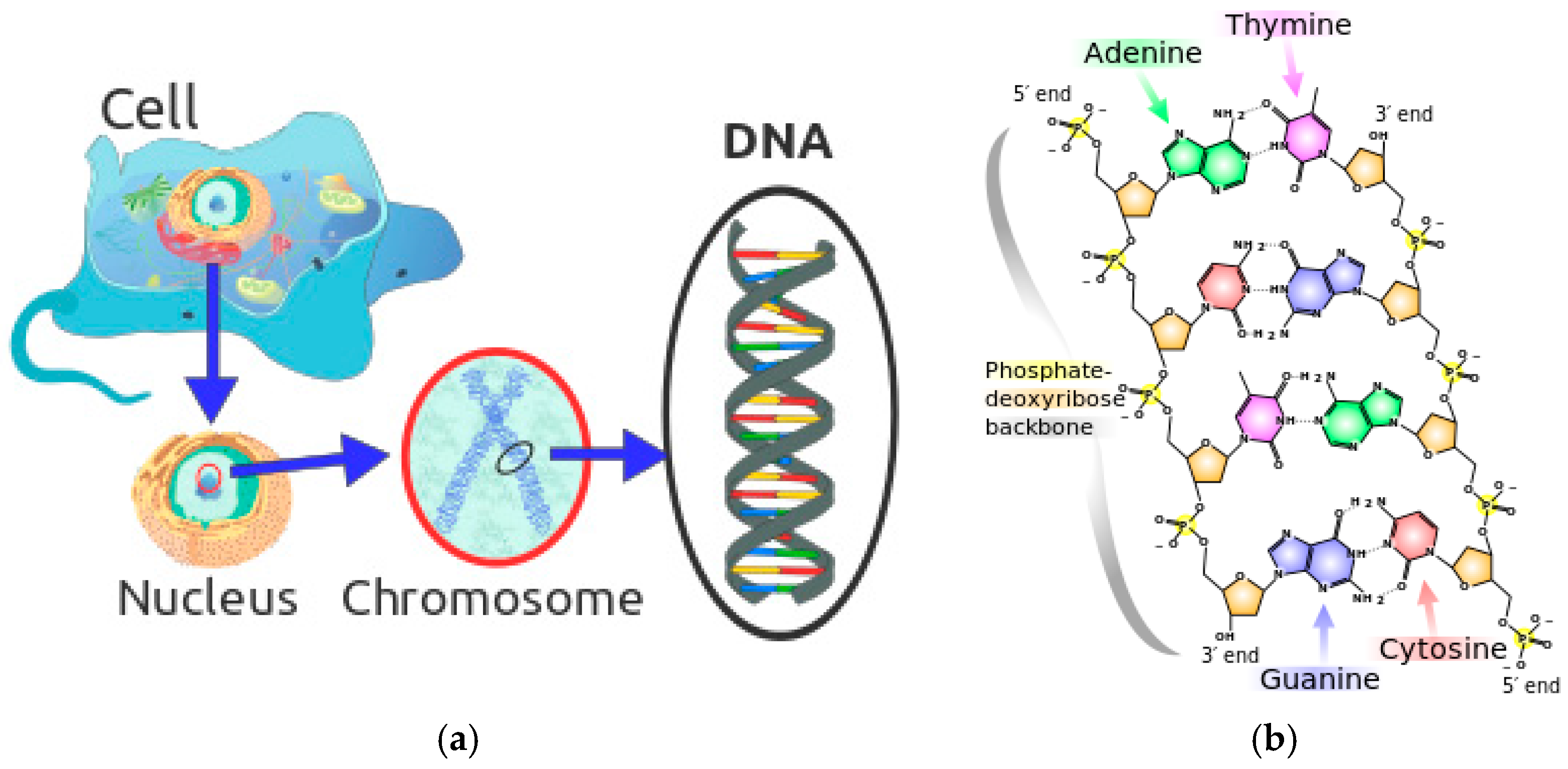
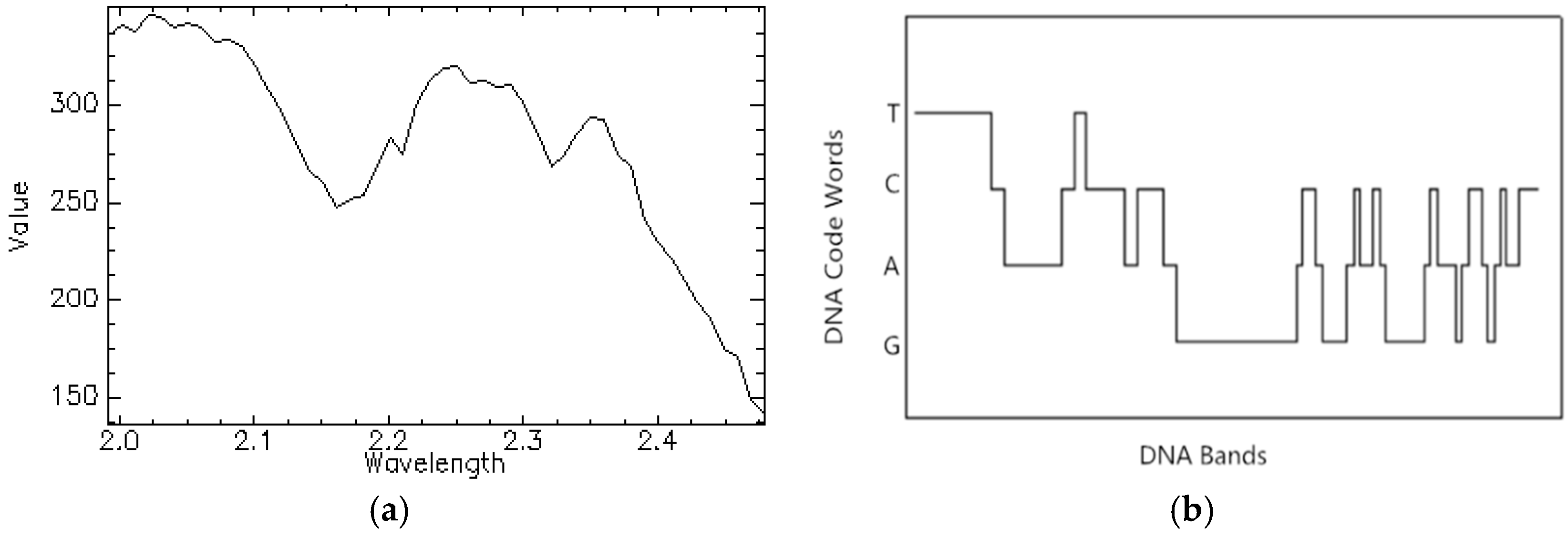
Recently, a novel classification strategy inspired by the artificial deoxyribonucleic acid (DNA) technology has been presented for hyperspectral remote sensing imagery [17,18,19,20]. As a branch of computational intelligence, artificial DNA encoding and matching (ADEM) method has the strong computing and matching capability to discriminate the tiny differences in DNA strands [21]. It can discriminate the tiny differences in DNA strands by DNA encoding and matching in the molecule layer. DNA encoding method in this classifier plays an important role. It not only reduces the influence of the noise caused by sunlight and weather but also takes both brightness and shape information into consideration [7]. In a word, it has been proven that ADEM can comprehensively compare the similarity of two spectra. However, there are some limitations in practice so that the classification result is affected. Because when all of the bands participate in the encoding procedure, data volume is expanded which may amplify redundancy. Moreover, the full-band comparison degrades the importance of key spectral bands carrying critical information in class separation [22].

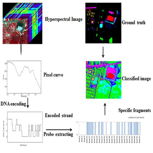
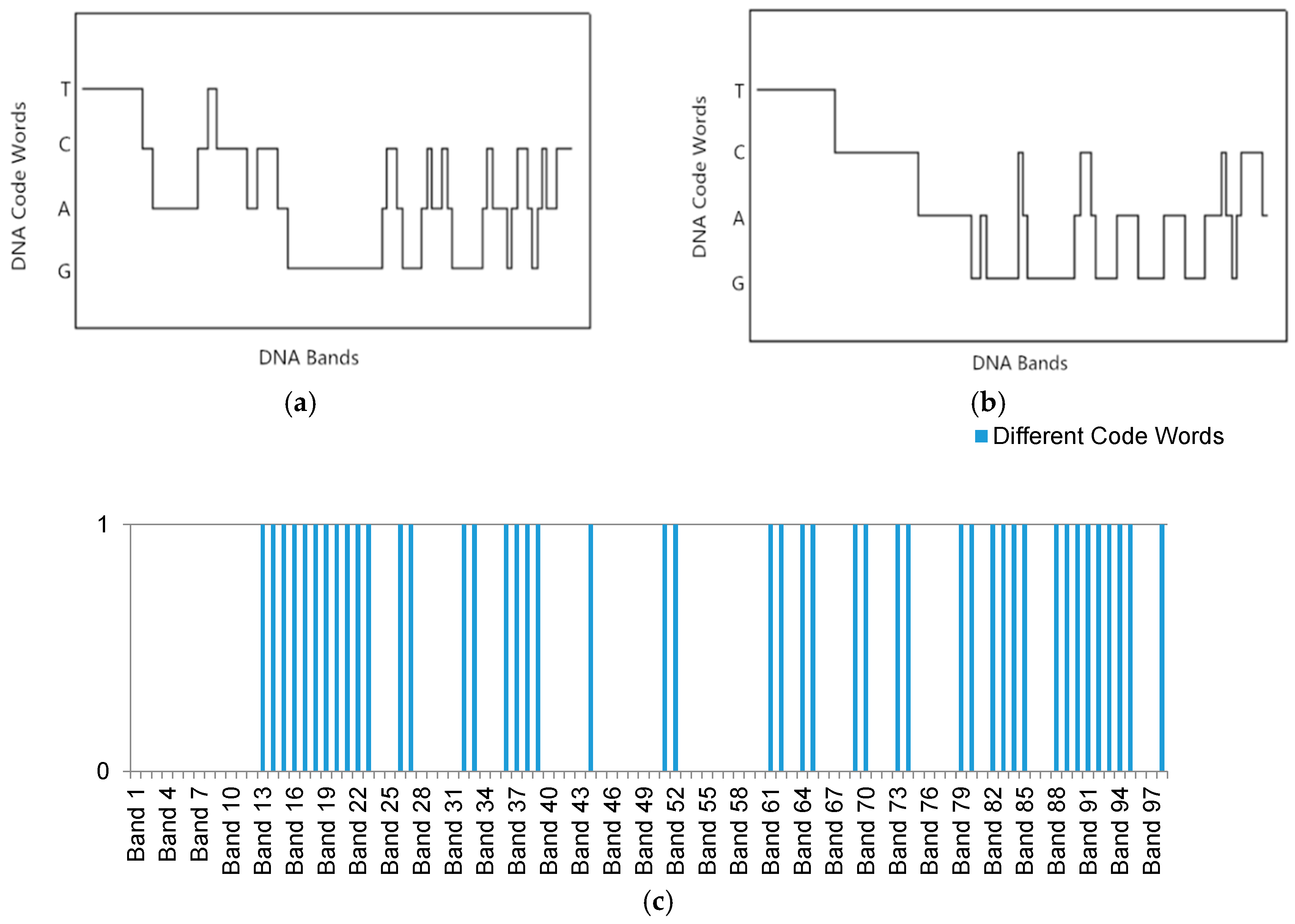
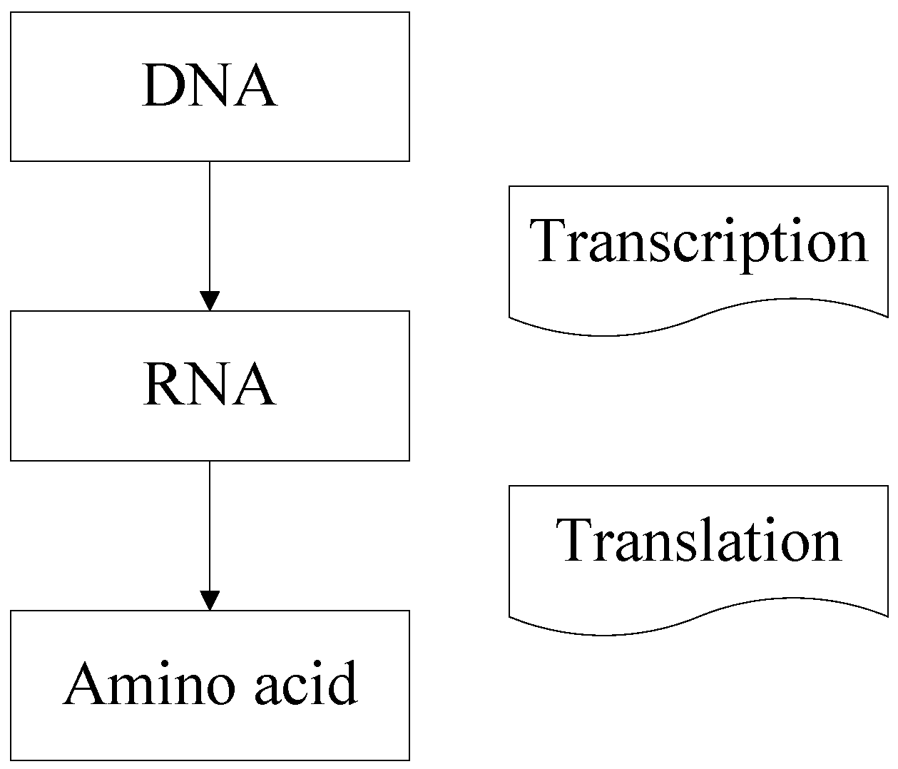
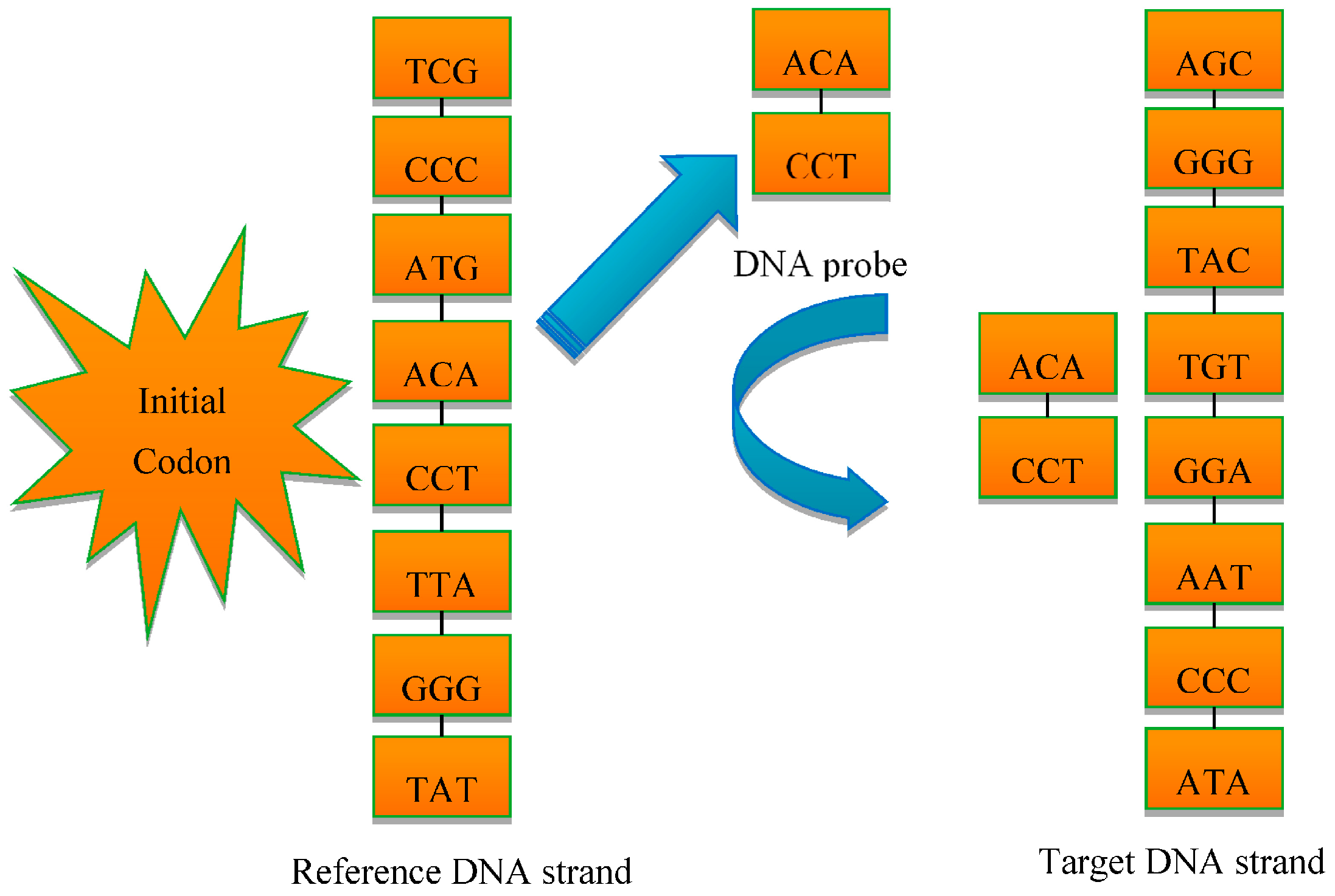
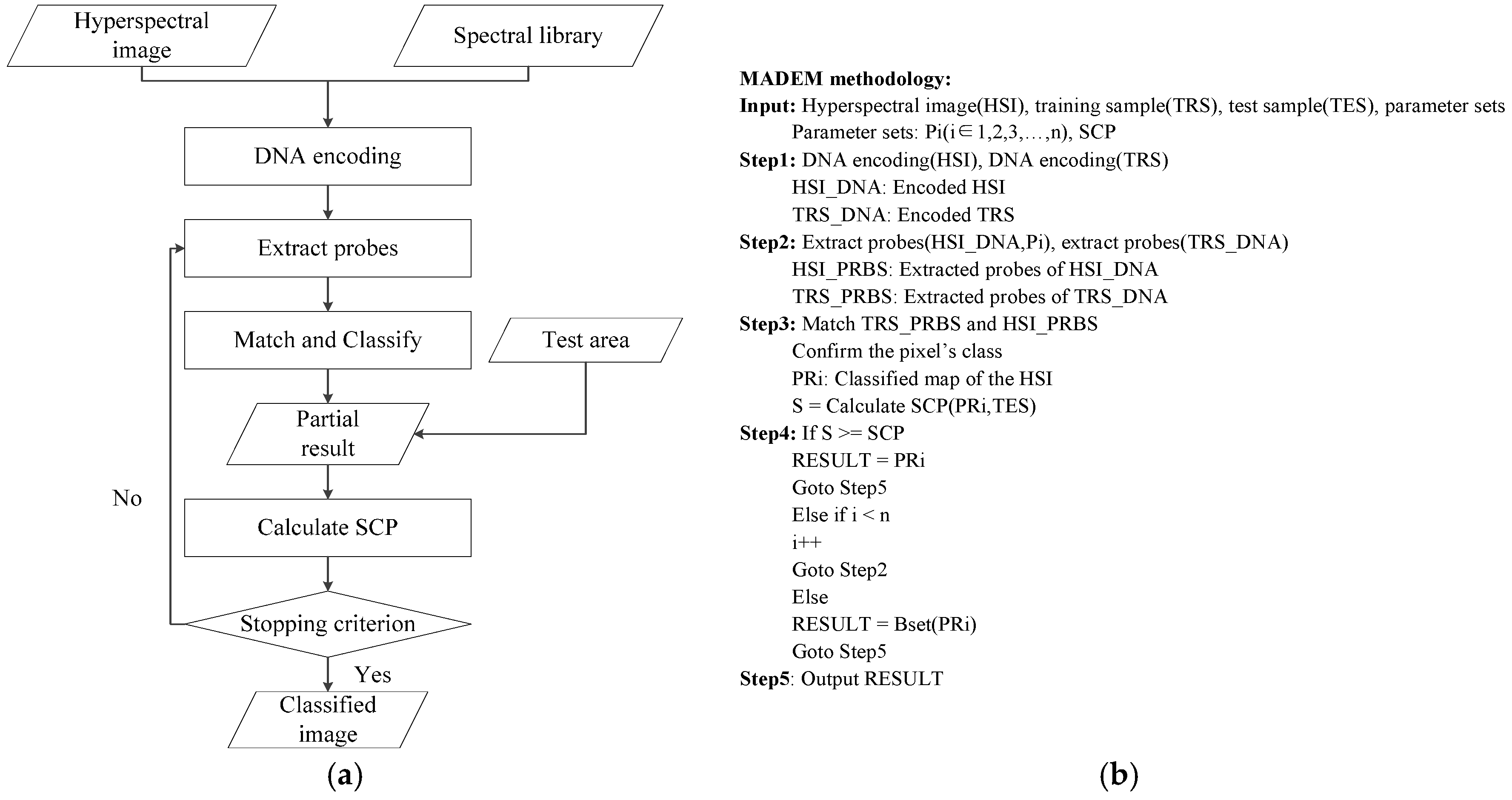
In order to overcome these shortcomings, a new multi-probe based artificial DNA encoding and matching (MADEM) method is proposed in this paper. The biggest difference between ADEM and MADEM is that the latter looks for and extracts the specific information/fragments of the encoded DNA strands, which can replace the full-encoded DNA strands for the matching and classification process in hyperspectral remote sensing imagery. In other words, MADEM aims at seeking out the temporal information of the encoded DNA strands. In this method, multiple probes, defined as the extracted specific fragments of the DNA strand, is put forward for HSI. They are the temporal information of the DNA strands and are used to copy genes and find the most characteristic element of a spectrum. It is well known that only genes can transfer the genetic information of creatures in biological sciences [23]. Differences in genes can lead to various lives. Thus, the probes, which represent unique fragments of encoded strand, can be extracted to distinguish different spectra. This new method can help to improve the district division by discriminating spectra of different land covers. Meanwhile, the impact of redundant bands can be reduced. Generally, the number of probes is varied due to numerous genes on DNA strands. The probes are extracted randomly and do not share cross regions during the process. In order to generate the most effective probes, the algorithm can be iterated many times to achieve the best solution. The extracted probes provide a more precise discrimination of spectrums, which is favorable for matching and classification process.

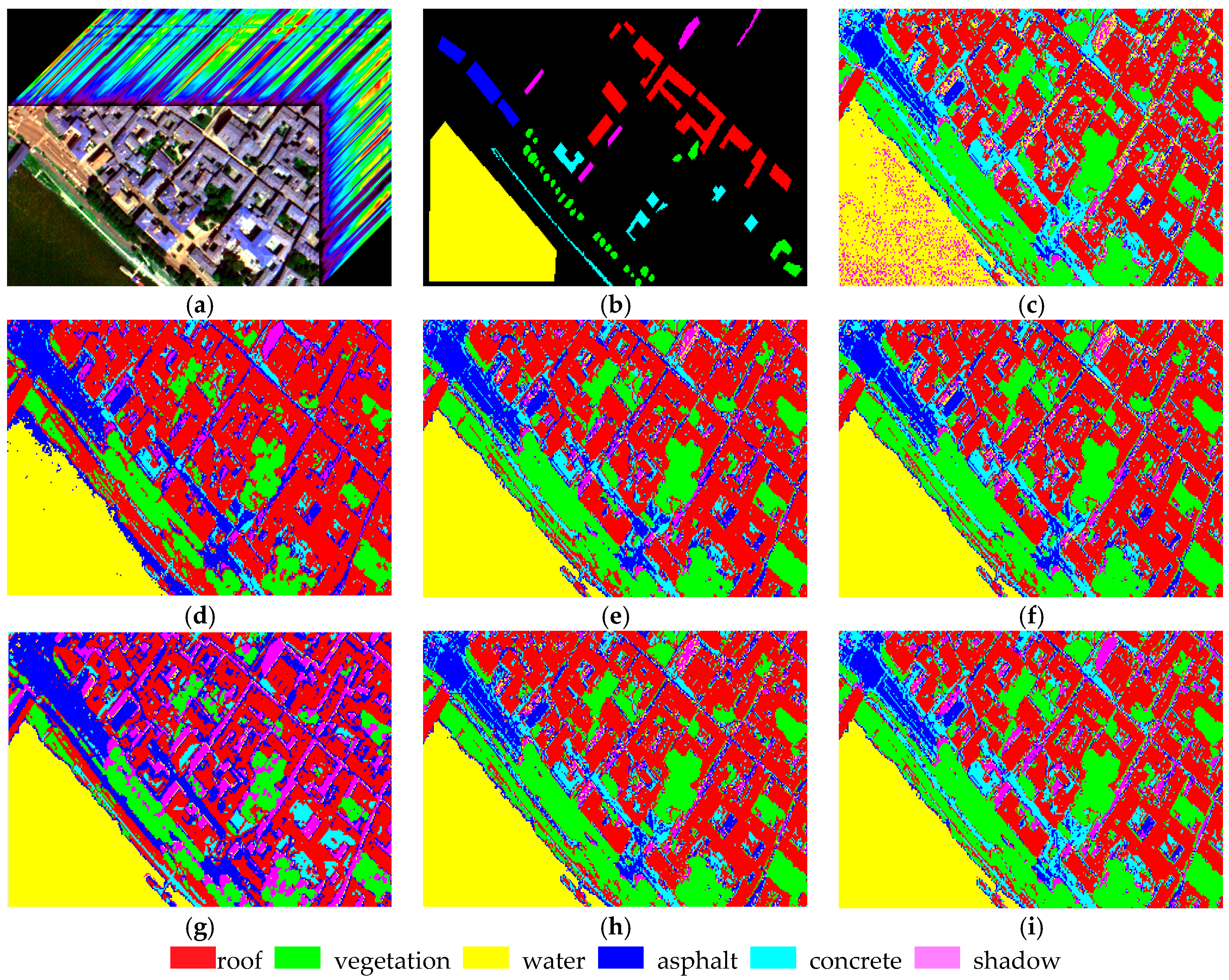
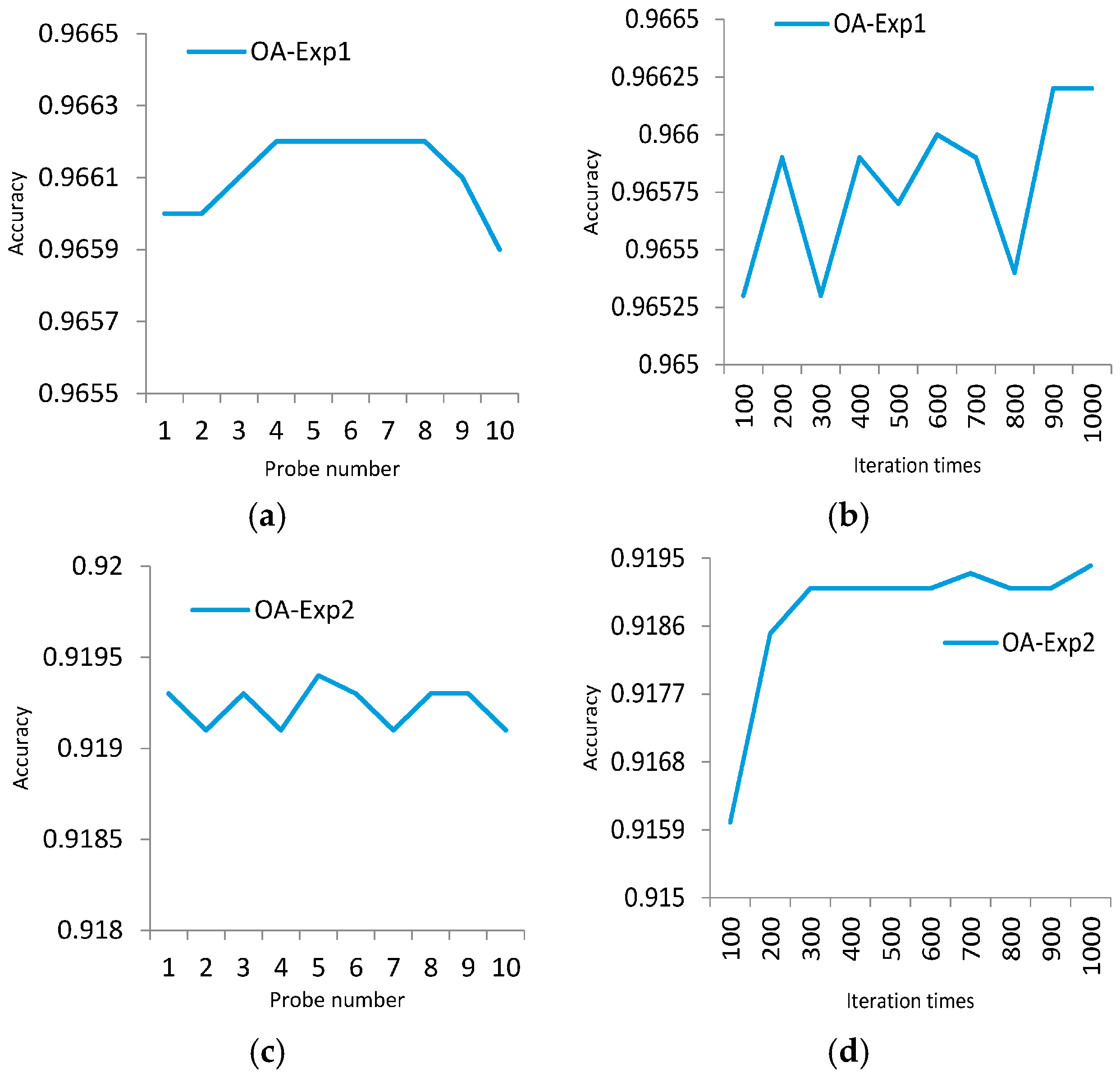
The rest of this paper is organized as follows: Section 2 introduces the background of biological DNA and DNA encoding method for hyperspectral remote sensing data. Section 3 provides the background of DNA probe technology and describes the multi-probe selection strategy in detail. Section 4 shows two experiments using several traditional algorithms compared with MADEM. The computational complexity of these methods is provided in Section 5. Finally, conclusion is drawn in Section 6.

2. DNA Encoding

2.1. The Basic Theory of DNA

As showen in Figure 1a, DNA exists in creature chromosome, and it contains key genetic information of creatures. However, for human beings, 99.99% of human DNA sequences are the same. Some specific fragments in DNA, called genes, enable to distinguish one individual from another [24]. DNA strands consist of four types of bases: thymine (T), adenine (A), cytosine (C), and guanine (G), as shown in Figure 1b. Not all of the bases on the DNA strands have direct influence on lives, which means only a few pieces of DNA strands, i.e., genes, play a critical role in biological difference [25]. Genes consist of four types of original bases. Genes make creatures different from each other by conveying genetic information while non-genomic sequences have structural purposes.

As shown in Figure 2, genetic information stored on the DNA strand is transcribed to ribonucleic acid (RNA) strand. After the RNA has been transcribed, the RNA translates the genetic information to amino acids, which are the composition of proteins [28]. Different combinations of proteins determine different kinds of creature. On the RNA strand, three adjacent bases are called codon, on which the type of amino acid depends. There are 61 kinds of codons including two kinds of initial codons, in which the amino acid starts to be translated. In sum, genes on DNA strand determine the differences of creatures through two steps: transcription and translation.

Although DNA strands of different creatures are overall similar, some key parts are significantly different. It is these key parts that lead to the variety of lives. If these key parts can be located, the most critical information for discrimination can be extracted.

2.2. The DNA Encoding Method

A DNA strand can be likened to an array of four different symbols {T, C, A, G}, meaning DNA strands can be encoded by these four code words, which is enough to describe the information of DNA by different combinations [29]. Considering the similarity of DNA strand and spectrum, i.e., they are both high dimensional data, DNA encoding method was utilized for hyperspectral data. After DNA encoding, spectra, i.e., image pixels, are encoded to DNA strands consisting of {T, C, A, G}. To extract comprehensive information of spectra, encoded DNA strand must include the brightness and shape information of the spectra simultaneously [30]. Spectral DNA encoding is illustrated in Figure 3. Figure 3a shows the original spectral curve of alunite mineral, and Figure 3b shows the DNA encoded alunite mineral. It is clearly shown that DNA encoding method can well describe the brightness and shape information.

2.2.1. DNA Encoding for Spectral Brightness Information

The continuous-valued reflectance must be converted into four types of gradients, and then the spectra can be encoded to an array of DNA code words according to the gradients. For the i-th band of the spectral signature, defined as ${\mathrm{y}}^{\mathrm{i}}$, three thresholds separate the spectral value into four gradients. After the spectral values of the i-th band are compared with the thresholds, it is encoded to the corresponding code words according to the gradients. The thresholds are calculated as follows. First, the middle threshold marked as ${\mathrm{T}}_{\mathrm{middle}}$ can be acquired, and then, the other two thresholds marked as ${\mathrm{T}}_{\mathrm{lower}}$ and ${\mathrm{T}}_{\mathrm{higher}}$ can be calculated based on ${\mathrm{T}}_{\mathrm{middle}}$ [19,20].

$${\mathrm{T}}_{\mathrm{middle}}=\mathsf{\rho }{\displaystyle \sum _{\mathrm{i}=1}^{\mathrm{Nb}}{\mathrm{y}}^{\mathrm{i}}}/\mathrm{Nb}$$

(1)

$${\mathrm{T}}_{\mathrm{higher}}={\displaystyle \sum _{\mathrm{i}=1}^{\mathrm{Nb}}\mathrm{Bigger}({\mathrm{y}}^{\mathrm{i}})}/\mathrm{k}$$

(2)

$${\mathrm{T}}_{\mathrm{lower}}={\displaystyle \sum _{\mathrm{i}=1}^{\mathrm{Nb}}\mathrm{Smaller}({\mathrm{y}}^{\mathrm{i}})}/\mathrm{p}$$

(3)

where $\mathrm{Bigger}({\mathrm{y}}^{\mathrm{i}})=\{\begin{array}{ll}{\mathrm{y}}^{\mathrm{i}}& \mathrm{if}{\mathrm{y}}^{\mathrm{i}}\ge {\mathrm{T}}_{\mathrm{middle}}\\ 0& \text{else}\end{array}$, $\mathrm{Smaller}({\mathrm{y}}^{\mathrm{i}})=\{\begin{array}{ll}{\mathrm{y}}^{\mathrm{i}}& \mathrm{if}{\mathrm{y}}^{\mathrm{i}}<{\mathrm{T}}_{\mathrm{middle}}\\ 0& \text{else}\end{array}$, and Nb is the number of number of the image bands. k is the number of bands whose value are bigger than ${\mathrm{T}}_{\mathrm{middle}}$, p is the number of bands whose value is smaller than ${\mathrm{T}}_{\mathrm{middle}}$ and $\mathsf{\rho }$ is the adaptive coefficient of DNA brightness encoding with domain value (0.5, 1.0). Since different $\mathsf{\rho }$ can lead to different code, the range of $\mathsf{\rho }$ has to be turned. The encoding method is based on the four gradients:

$$\mathrm{DN}{\mathrm{A}}_{\mathrm{i}}^{\mathrm{brightness}}=\{\begin{array}{l}\mathrm{G},\mathrm{if}{\mathrm{y}}^{\mathrm{i}}\in [{\mathrm{y}}_{\min },{\mathrm{T}}_{\mathrm{lower}})\\ \mathrm{A},\mathrm{if}{\mathrm{y}}^{\mathrm{i}}\in [{\mathrm{T}}_{\mathrm{lower}},{\mathrm{T}}_{\mathrm{middle}})\\ \mathrm{C},\mathrm{if}{\mathrm{y}}^{\mathrm{i}}\in [{\mathrm{T}}_{\mathrm{middle}},{\mathrm{T}}_{\mathrm{higher}})\\ \mathrm{T},\mathrm{if}{\mathrm{y}}^{\mathrm{i}}\in [{\mathrm{T}}_{\mathrm{higher}},{\mathrm{y}}_{\max }]\end{array}$$

(4)

where ${\mathrm{y}}_{\min }$ means the minimum value of the spectral curve, and the ${\mathrm{y}}_{\max }$ means the maximum value of it.

2.2.2. DNA Encoding for Spectral Shape Information

Only considering spectral brightness may not well discriminate different land covers. The shape information has to be encoded. There are many approaches to describe spectral shape. For example, the change of spectral curve of two adjacent bands can reflect the shape, but it can only be encoded to three kinds of code words. Three adjacent bands can provide nine kinds of spectral shape change. Nevertheless, more than three adjacent bands provide more kinds of spectral shape change. It is not efficient for encoding process. To describe shape details, three adjacent bands can be appropriate for DNA encoding. Assume that $\mathrm{y}={\{{\mathrm{y}}_1,{\mathrm{y}}_2,{\mathrm{y}}_3,\mathrm{\dots },{\mathrm{y}}_{\mathrm{Nb}}\}}^{\mathrm{T}}$ represents a hyperspectral signature, and Δ represents the spectral value tolerance. Then spectral shape details can be encoded as follows [19,20]:

Type 1: if $\left|{\mathrm{y}}^{\mathrm{i}}-{\mathrm{y}}^{\mathrm{i}-1}\right|\le \mathsf{\Delta }\text{ and }\left|{\mathrm{y}}^{\mathrm{i}+1}-{\mathrm{y}}^{\mathrm{i}}\right|\le \mathsf{\Delta }$

Type 2: if $(\left|{\mathrm{y}}^{\mathrm{i}}-{\mathrm{y}}^{\mathrm{i}-1}\right|\le \mathsf{\Delta }\text{ and }\left|{\mathrm{y}}^{\mathrm{i}+1}-{\mathrm{y}}^{\mathrm{i}}\right|>\mathsf{\Delta })$ or $(\left|{\mathrm{y}}^{\mathrm{i}}-{\mathrm{y}}^{\mathrm{i}-1}\right|>\mathsf{\Delta }\text{ and }\left|{\mathrm{y}}^{\mathrm{i}+1}-{\mathrm{y}}^{\mathrm{i}}\right|\le \mathsf{\Delta })$

Type 3: if $({\mathrm{y}}^{\mathrm{i}}-{\mathrm{y}}^{\mathrm{i}-1}<-\mathsf{\Delta }\text{ and }{\mathrm{y}}^{\mathrm{i}+1}-{\mathrm{y}}^{\mathrm{i}}<-\mathsf{\Delta })$ or $({\mathrm{y}}^{\mathrm{i}}-{\mathrm{y}}^{\mathrm{i}-1}>\mathsf{\Delta }\text{ and }{\mathrm{y}}^{\mathrm{i}+1}-{\mathrm{y}}^{\mathrm{i}}>\mathsf{\Delta })$

Type 4: if $({\mathrm{y}}^{\mathrm{i}}-{\mathrm{y}}^{\mathrm{i}-1}<-\mathsf{\Delta }\text{ and }{\mathrm{y}}^{\mathrm{i}+1}-{\mathrm{y}}^{\mathrm{i}}>\mathsf{\Delta })$ or $({\mathrm{y}}^{\mathrm{i}}-{\mathrm{y}}^{\mathrm{i}-1}>\mathsf{\Delta }\text{ and }{\mathrm{y}}^{\mathrm{i}+1}-{\mathrm{y}}^{\mathrm{i}}<-\mathsf{\Delta })$

The $\mathsf{\Delta }$ can be set as follows:

$$\mathsf{\Delta }=\mathsf{\theta }(\frac{1}{\mathrm{Nb}-1}){\displaystyle \sum _{\mathrm{i}=2}^{\mathrm{Nb}}({\mathrm{y}}^{\mathrm{i}}-{\mathrm{y}}^{\mathrm{i}-1})}$$

(5)

where $\mathsf{\theta }$ is the shape adaptive coefficient. The DNA encoding technique is used to capture spectral texture feature changes in three consecutive adjacent bands. If 1 < i < $\text{Nb}$, we can define the DNA shape details code words ${\text{DNA}}_{\mathrm{i}}^{\text{Shape}}$ as:

$$\mathrm{DN}{\mathrm{A}}_{\mathrm{i}}^{\mathrm{shape}}=\{\begin{array}{ll}\mathrm{T},& \mathrm{i}\mathrm{f}{\mathrm{y}}^{\mathrm{i}}\mathrm{i}\mathrm{s}\mathrm{T}\mathrm{y}\mathrm{p}\mathrm{e}1\\ \mathrm{C},& \mathrm{i}\mathrm{f}{\mathrm{y}}^{\mathrm{i}}\mathrm{i}\mathrm{s}\mathrm{T}\mathrm{y}\mathrm{p}\mathrm{e}2\\ \mathrm{A},& \mathrm{i}\mathrm{f}{\mathrm{y}}^{\mathrm{i}}\mathrm{i}\mathrm{s}\mathrm{T}\mathrm{y}\mathrm{p}\mathrm{e}3\\ \mathrm{G},& \mathrm{i}\mathrm{f}{\mathrm{y}}^{\mathrm{i}}\mathrm{i}\mathrm{s}\mathrm{T}\mathrm{y}\mathrm{p}\mathrm{e}4\end{array}$$

(6)

As the brightness and shape features have been encoded, the whole DNA strands of a spectrum can be represented as follows:

$${\mathrm{DNA}}^{\mathrm{code}}=\{{\mathrm{DNA}}_1^{\mathrm{brightness}},{\mathrm{DNA}}_2^{\mathrm{brightness}},\mathrm{\dots },{\mathrm{DNA}}_{\mathrm{Nb}}^{\mathrm{brightness}},{\mathrm{DNA}}_1^{\mathrm{shape}},\mathrm{\dots },{\mathrm{DNA}}_{\mathrm{Nb}-2}^{\mathrm{shape}}\}$$

(7)

The number of spectral shape code words is Nb-2, because three consecutive adjacent bands determine code words and the last two bands cannot extract the shape information.

3. The Multi-Probe Based Artificial DNA Encoding and Matching Method

The proposed MADEM algorithm is mainly made up of the DNA encoding method and the DNA multi-probe extracting strategy. The former transforms spectral information into DNA information, and the latter optimizes the DNA information through selecting specific fragments of DNA strand. In this section, the DNA probe and multi-probe extracting approaches will be introduced.

3.1. The DNA Probe Technology

In 1975, DNA probe technology was first proposed with in the field of biology by South. Currently, the technology has become the basic technology of modern molecular biology, and it has been improved and developed in many fields [30]. DNA probe technology is also called molecular hybridization technique. It utilizes the DNA molecule characteristics of degeneration, renaturation, and high accuracy of complementary base pairs. These characteristics allow DNA probe to be utilized to search the target DNA strands [30]. In practical applications, DNA probe technology can be used to quickly detect pathogens by using specific artificial single-stranded DNA fragment of the pathogens with radioactivity or biomarkers. The probe is a single-stranded RNA, which can detect the target DNA strand through testing the radiation after base pairing of the probe and the target DNA strand. Compared with the traditional method, DNA probe technology is fast and sensitive. Traditional methods spend several days or even weeks to finish once detection with low precision while DNA probe technology just spends one day with high precision. It is reported that DNA probe approach can detect ten viruses from one ton water [30,31].

Figure 4 shows the mechanism of DNA probe technology in biology. Every letter means a kind of base (thymine (T), adenine (A), cytosine (C), and guanine (G)). Every three bases make up a codon, such as the ACA and CCT in Figure 3, which is the basic unit of fragment of a DNA strand. DNA probe is some continuous sequences of the RNA strand. It must be specific to discriminate the target DNA strand from others. The DNA probe detecting process in biology field is expressed as follows: First, a probe is extracted from the reference DNA strand with specificity being assured. Then, many copies of the probe are synthesized for detection. Although it increases the time of detection, a precise result can be obtained by this contribution. The hybridization environment (such as water, proper temperature, enzyme and so on) of the probes and target DNA strands can help to perform the next step. Proper environment is conducive to detection efficiency. If the probes find the pairing bases, they match with each other, unless they are dissociative. Pairing rules are: (1) T matches G; and (2) C matches G. The dissociative probes are dissolved. Finally, the remaining DNA strands are tested. If there are biomarkers or radiation in the remaining strands, it means the target DNA strands are successfully detected.

3.2. The DNA Multi-Probe Extracting Strategy Based on Hyperspectral Remote Sensed Image

Based on this concept, it is possible for hyperspectral data to be recognized by special band sequences if DNA probes can be extracted. As shown in Figure 5, spectral curves of alunite (Figure 5a) and halloysite (Figure 5b) are both encoded to DNA strands. Furthermore, the difference of the DNA strands of alunite and halloysite can be represented in Figure 5c. The different code words are represented as “1” for blue, and the same code words are represented as “0” for white in the chart. It is clear that the different parts of the encoded DNA strands are some fragments, not all the DNA strands. Only some sequences on the DNA strand provide a distinction for different DNA strands, as does land cover spectrum: different land covers can be distinguished more precisely by specific fragments.

The proposed DNA multi-probe extracting strategy includes four steps: DNA encoding, multi-probe extracting, matching classification and parameter iteration. First, the hyperspectral image and spectral library are both encoded to DNA strands using Equations (1)–(7). The continuous spectra are converted to discrete values. After that, the multi-probe is extracted for matching classification from the DNA strands instead of the RNA strands. It is the core step of the proposed algorithm. For comparison of different matching classification performance, several groups of probe numbers are set by the user. Meanwhile, probes are selected randomly in order to extract specific probes to differentiate land covers, which means the starting positions and lengths of probes are decided randomly. The probe extraction strategy can reach the best selection result by iterating the process. To assure the validity of the probes, three rules are observed:

(1)

The starting positions of the probe, which means the initial codon in Figure 2, should be determined in the range of strands;

(2)

The length of the strands should not be beyond the strand length; and

(3)

Each probe should be selected from the strands, which is the probe selection rule.

In MADEM, the starting positions of the probes cannot be set by the user unless he or she knows the locations of the specific fragments. After the number of probes is set, the starting points are determined randomly. Rule 1 can obtain the starting positions of the probes and decreases the risk of human intervention at the same time. Rule 2 imposes some restrictions on the probe length because the probe extraction result is affected by the length of the probe, and that has a great impact on classification performance. If the probe is longer, more nonspecific fragments are contained in the probe. Furthermore, some probes are overlapped so that the comparison of spectrum is affected, which can decrease the classification accuracy. On the contrary, if the probe is shorter, some code words of the specific fragment may be ignored, which can lead to the typical information of classification is missing. For the above reasons, both the aspects decrease the classification accuracy. Thus, the proper probe length should be chosen based on Rule 2. Rule 3 assures the validity of probes. Random selection of start position and probe length may lead the probe extract beyond the strand rang. These kinds of probes are invalid and illegal, so Rule 3 puts the restriction on the selection process.

After probe extraction, match classification is carried out. Spectral match process aims at comparing the spectral similarity of the reference spectrum and a pixel spectrum. The similarity is defined the total AVD of each probe:

$$\mathrm{AVD}={\displaystyle \sum _{\mathrm{p}=1}^{\mathrm{Np}}{\displaystyle \sum _{\mathrm{i}=1}^{\mathrm{Lp}}\mathrm{f}({\mathrm{p}}_{\mathrm{i}}^1,{\mathrm{p}}_{\mathrm{i}}^2)}}/{\displaystyle \sum _{\mathrm{p}=1}^{\mathrm{Np}}\mathrm{Lp}}$$

(8)

where $\mathrm{Np}$ means the number of probes, $\mathrm{Lp}$ means the length of the pth probe, and $\mathrm{f}({\mathrm{p}}_{\mathrm{i}}^1,{\mathrm{p}}_{\mathrm{i}}^2)=\{\begin{array}{ll}1& \mathrm{if}{\mathrm{p}}_{\mathrm{i}}^1={\mathrm{p}}_{\mathrm{i}}^2\\ 0& \mathrm{else}\end{array}$. The result of calculation will be larger if the two spectra are more similar. The classification process can be carried out according to the match result. When a pixel has the largest similarity with a reference spectrum, the pixel will be classified to that class.

Due to random selection of probes of encoded DNA strands, the performance may not be stable. Iteration strategy contains two aspects: iteration and stopping criterion. The iteration increases the probability of getting the proper probes by increasing the selection times. During the process, there should be a measure evaluating once the classification result will be satisfied. In this paper, it is called stopping criterion parameter (SCP).

$$\mathrm{SCP}={\mathrm{Kappa}}_{\mathrm{i}}$$

(9)

$${\mathrm{Kappa}}_{\mathrm{i}}=\frac{\mathrm{N}{\displaystyle \sum {\mathrm{m}}_{\mathrm{kk}}}-{\displaystyle \sum ({\mathrm{m}}_{\mathrm{k}+}{\mathrm{m}}_{+\mathrm{k}})}}{{\mathrm{N}}^2-{\displaystyle \sum ({\mathrm{m}}_{\mathrm{k}+}{\mathrm{m}}_{+\mathrm{k}})}}$$

(10)

where ${\mathrm{m}}_{\text{kk}}$ is the number of observations in row k and column k of the confusion matrix, which is calculated by test area and the i-th classified map; ${\mathrm{m}}_{\mathrm{k}+}$ and ${\mathrm{m}}_{+\mathrm{k}}$ are the marginal totals for row k and column k of the confusion matrix; and N is the total number of observations. The value of SCP equals the kappa of the i-th iteration calculating result. This measure can well evaluate the classification performance.

The entire algorithm is illustrated in Figure 6a. In Step 1, the image and the spectral library are encoded to DNA strands. In Step 2, DNA probes are extracted from the encoded DNA strands of spectral library and image based on some extraction rules mentioned previously. In Step 3, classification is carried out based on the AVD of reference probes and the pixel probes. In Step 4, the CSP is calculated from the local classification result and test samples. In Step 5, the iteration stopping criterion is tested if the criterion is reached, the algorithm is terminated; otherwise, repeat Steps 2–5. More details are shown in Figure 6b, including the pseudo-code of MADEM. The stopping criterion contains two aspects: if the SCP of the partial result of the iteration reaches the artificially set threshold, the iteration will end; and, if the iteration time reaches the artificially set value, the iteration will end. Furthermore, the result of bet SCP will be output.

4. Experiment

The proposed MADEM algorithm was tested on two hyperspectral images. Comparison with some traditional spectral matching algorithms are given, including binary coding (BC) method [7], spectral correlation match (SCM) method [11], spectral angle mapping (SAM) [10], cross correlation spectral match (CCSM) method [12], support vector machine (SVM) [4], and artificial DNA encoding and matching (ADEM) method [19]. The hardware and software parameters are followed: laptop of Acer, Intel(R) Core(TM) i5-2430M [email protected] MHz, 6 G RAM, Windows 7 OS, Visual Studio 2010 IDE.

4.1. Experiment 1

The image data in this experiment were acquired by the airborne ROSIS sensor at Pavia urban area, north Italy. The size of the whole data set is 1400 × 512 pixels, and the experimental area is a subset of 323 × 187 in the experiment. The data set was provided by the Data Fusion Technical Committee (DFTC) [32]. The original 115 bands over 0.43 to 0.86 μm and the spectral resolution is 4 nm. Thirteen bands were removed due to low signal-to-noise ratio. The spatial resolution is 1.3 m. The ground-truth image and the list of classes and their corresponding numbers of samples are shown in Figure 7 and

Table 1. Training and testing pixels.

Experimental Samples	Roof	Vegetation	Asphalt	Water	Concrete	Shadow	Total
training samples	20	27	13	46	7	6	119
testing samples	2306	791	704	7269	772	400	12,242

, respectively. In order to better test the practicality of MADEM, only 119 training samples of the image are chosen. If the small training size can lead to a satisfactory classification result, the proposed algorithm will be proven more robust and better than the other methods. Figure 7a shows the false-color image with band 10, 20 and 61. Figure 7b shows the ground truth, where the six classes are: roof, vegetation, asphalt, water, concrete, and shadow. Figure 7c–i shows the classification results of the seven classifiers.

Parameters of the algorithm are set as follows. The brightness adaptive coefficient of DNA encoding and the shape adaptive brightness coefficient are both set as 1.0. The SVM applies a radial basis function as the kernel function and a cross-validation approach to determine the optimal values of the parameters [33]. The parameter of probe number is set as 5. The iteration time of the iteration calculating is set as 1000. The artificially SCP is set as 0.99. Table 1 shows the training and testing pixels of the experiment 1. In the aspect of visual comparison, BC produces the worst visual result. It can distinguish the concrete road, but cannot recognize shadows. Moreover, BC method misclassified some water pixels as shadows. SAM can well distinguish most classes except concrete road and asphalt road. The result of SAM has clear eades of different land covers, but it misclassified too many concrete road and vegetation pixels. The performance of SCM is better than SAM. SCM can recognize more concrete pixels than SAM. The result of CCSM is similar to that of SCM. The result of SVM shows clear edges of different land covers and it can discern the shadows well. However, SVM ignored many concrete road and buildings. Compared to the result of MADEM, ADEM gets less shadow pixels right identified. The result of MADEM can discern the vegetation well, and it can get an excellent division of all the land covers.

The confusion matrix is in Figure 8. The kappa coefficient, overall accuracy (OA) and process time are listed in

Table 2. Overall accuracy and kappa coefficient of all classifiers.

Method	BC	SAM	SCM	CCSM	SVM	ADEM	MADEM
overall accuracy (%)	86.53	94.73	94.87	94.97	94.63	95.06	96.62
kappa coefficient (%)	79.06	91.21	91.38	91.53	91.10	91.69	94.35

. From Figure 8, it is noticed that every classifier, except BC and SAM, can 100% recognize the water correctly. As for vegetation, all classifiers can 100% recognize it correctly. From Table 2, it is clear that the performance of BC is the worst. The performance of SAM, SCM, CCSM and SVM are similar in this experiment. MADEM provides the best result with the kappa of 94.35% and OA of 96.62%, with a gain of 3.25% and 1.99% over SVM and with a gain of 2.66% and 1.56% over ADEM.

BC cannot distinguish the water and shadow well because the two spectral curves are close in spectral brightness. BC discriminates land covers through binary codes of spectral brightness without extracting discriminative information in spectral shapes. SAM, SCM, and CCSM are based on spectral shape. They generate better classification than BC because the spectral curves of the land covers in this experiment are more important. The result of CCSM is better than SAM and SCM because the RMS can take the skewness and crest of the spectral curves into account. SVM has the similar performance with the former traditional methods mainly because of the small training samples. This affects the learning process of SVM, while it has little influence to the DNA method. ADEM utilizes the brightness and shape information of the spectral curves to recognize the land covers, so its performance is better than the traditional algorithms. From the experiment, it is clear that MADEM has a gain over SVM and ADEM. That means the proposed algorithm can get a better performance than the traditional ADEM and SVM method in this experiment.

4.2. Experiment 2

Another hyperspectral remote sensing image was also used: the urban data set captured by the HYDICE sensor in October 1995, and 210 bands are included. The objects in this image are more diverse and include different types of roofs and roads, posing a greater challenge for the classifiers than the experiment 1. It is located at Copperas Cove, near Fort Hood, Texas, U.S., with a size of 307 × 307. The spectral resolution is 10 nm and the spatial resolution is 2 m. The main classes in this area include mall roof (roof-1), house roof (roof-2), tree, concrete, grass and asphalt. In addition, due to the low solar altitude, trees and houses cast long shadows on the ground [34]. The ground truth image and the list of classes and their corresponding numbers of samples for this experimental data set are described in Figure 9 and

Table 3. Training and testing pixels.

Experimental samples	Roof-1	Tree	Concrete	Roof-2	Grass	Asphalt	Shadow	Total
training samples	8	8	10	10	8	14	10	68
testing samples	2006	1592	985	698	1326	1985	245	8837

, respectively. Before classification, bands 103–108, 139–152, and 208–210 are removed because they are regarded as noisy or water-absorption bands [35,36]. Similar to the Pavia urban area data set, the same strategy was used to separate the ground truth into the training samples and test samples.

In the MADEM, the parameters of probe number and iteration time are set as 8 and 900, respectively. The artificially SCP is still set as 0.99. The parameters of SVM are set same as the experiment 1. The false-color image is shown in Figure 9a. Figure 9b shows the ground truth of the experimental data. Figure 9c–i shows the classification results of the seven classifiers. The parameters are set as the experiment 1 in the algorithm process. Table 3 shows the training and testing samples of the experiment 2. According to Figure 9, visual comparisons demonstrate that the result of BC contains plenty of misclassifications of the land covers, and many pixels in the grass area are misclassified to tree. SAM cannot well separate the asphalt road and concrete road, and it misclassifies grass and concrete. The results of SCM and CCSM are similar, and both better than the result of SAM. The results of SCM and CCSM contain many pixels of tree and grass that are misclassified to concrete. SVM outperforms the aforementioned classifiers, and it can provide clear edges of different land covers. ADEM can well separate many land covers except grasses. MADEM yields the best classification result. The result of MADEM contains least misclassifications, and the edges of different land covers are sharp-edged.

From the Figure 10 and

Table 4. Overall accuracy and kappa coefficient of all classifiers.

Method	BC	SAM	SCM	CCSM	SVM	ADEM	MADEM
overall accuracy (%)	76.07	79.35	85.24	85.83	89.88	90.03	91.94
kappa coefficient (%)	70.62	75.24	82.14	82.87	87.78	87.86	90.21

, the performance of BC is the worst, again. SAM is better than BC. The results of SCM and CCSM are close and much better than the result of BC and SAM. SVM and ADEM perform better than the former traditional methods, but worse than MADEM. BC is based on spectral brightness, so it cannot distinguish grasses, concrete road and trees. The spectral signatures of asphalt road and roof-2 have similar shapes, so SAM, SCM, CCSM and even SVM misclassify asphalt road and roof-2. The result of ADEM is better mainly because the DNA encoded strands can well extract the brightness and shape information. Simultaneously, MADEM offers the best classification accuracy than the aforementioned algorithms. MADEM improves the kappa from 70.62% to 91.94% from the Table 4.

5. Computational Complexity Analysis

The computational complexity, also called calculation times and space cost of the computer, of the contrastive methods are provided in this section. As shown in

Table 5. Computational complexity of the algorithms.

Method	Calculation Times	Space Cost (Byte)
BC	2LSB + 2NB + NSLB + SLN	LBS + NB + 4NLS + SL
SAM	NSL${\mathrm{B}}^2$ + SLN	4(LBS + NB + 2B + NLS) + SL
SCM	NSL${\mathrm{B}}^2$ + SLN	4(LBS + NB + 2B + NLS) + SL
CCSM	21NSL${\mathrm{B}}^2$ + 2SLN	4(LBS + NB + 2B + 42 + NLS) + SL
SVM	8SLB + 6P + 10N + ${\mathrm{N}}^3+{\mathrm{N}}^2$ + 9SL + I(${\mathrm{N}}^2$ + 2N + 2P)	$\propto$ I, P, B, S, L, N
ADEM	6NB + 6SLB + 2SLNB + SLN	2(LBS + NB + 2NLS) + SL
MADEM	6NB + 6SLB + I(NPB + PBSL + NBSL + 2SLN)	2(LBS + NB + 2NLS) + SL + 4I

, BC has the least calculation times and space cost because of the simple encoding strategy. SAM and SCM have the same calculation times and they both cost more space than BC. CCSM has an iteration of getting spectral correlation 21 times. Thus, it needs more space to store the iteration result. As for SVM, because of its complex calculating process, the cross-validation and classification process contribute the most of the calculation times. The space cost of SVM is related to iteration times, band number, image size and class number. In the two DNA encoding methods, ADEM and MADEM have the same part of calculation time (6NB + 6SLB), mainly including the threshold calculation of T middle, T higher and T lower. The extra iteration process of ADEM and MADEM cost 2SLNB + SLN and I(NPB + PBSL + NBSL + 2SLN) times, respectively. Besides, they have the similar space cost.

Mathematical variables are defined as follows. S, the samples of the HSI; L, the lines of the HSI; B, the bands of the HSI, N, the number of the classes; P, the probe number in MADEM; and I, the iteration times of SVM and MADEM.

Based on the above analysis, the actual time costs of all classifiers in the two experiments are listed in

Table 6. Time costs of all classifiers in the two experiment.

Time (ms)	BC	SAM	SCM	CCSM	SVM	ADEM	MADEM
Experiment 1	2574	3572	3932	42,932	38,392	12,520	17,145
Experiment 2	3962	4961	4821	74,241	44,397	9953	12,543

. It should be noted that SAM, SCM, SVM and CCSM are performed with float-type data of the original image, while the other spectra encoding based classification methods, such as BC, ADEM and MADEM, are performed with the byte-type data transformed. BC is the fastest algorithm in the two experiments because the calculation time and space cost are both the smallest. SAM and SCM both cost more than BC and have the similar time. CCSM is the slowest algorithm because of its long iteration. In addition, the calculation of CCSM is based on float-type data, which will be more complex than byte-type data. SVM also costs much time because it contains a parameter optimization process. After parameter optimization, SVM reconstruct itself to classify the land covers. ADEM and MADEM both cost more time than BC, SAM and SCM since they have the DNA encoding process, but little than SVM and CCSM. When the image size is large, they can release more computational memory stress than other non-encoding algorithms. The probe extraction iteration of MADEM can lead to a little more calculation time than ADEM, but the time cost is still acceptable.

Since the computational complexity of MADEM is affected by the iteration time (I) and probe number (P), it is necessary to analyze the effect of setting these parameters when running the MADEM algorithm. In the two experiments, the parameters of probe number are both set from 1 to 10. Furthermore, the iteration time are both set from 100 to 1000 with the step length of 100. The overall accuracies (OA) of the two experimental images based on above two factors are shown in Figure 11.

As can be seen in Figure 11, the best performance appears when the probe number is 5 and the iteration time is 1000 in experiment 1. Furthermore, the best performance appears when the probe number is 8 and the iteration time is 900 in experiment 2. It has been found that the line chart of OA based on two factors both present vibratory. However, the differences in the accuracies among different parameter setups are very small. For probe number analysis, the difference between overall accuracy of the best and the worst classifications is near 0.03% for both case studies. For iteration time analysis, these differences are almost 0.08% and 0.3% for the two case studies. Thus, the conclusion can be drawn that, although the computational complexity of MADEM is more complex than the others, this kind of complexity can be reduced by decreasing the probe number and iteration times, which means, in this experiment, MADEM can reach an expectable result without more iteration and probe numbers.

6. Conclusions

In this paper, a new algorithm called MADEM is proposed for hyperspectral remote sensing imagery. MADEM can capture the rich information of spectral brightness and shape, which are both important for the spectral matching and discrimination process. It aims at finding separable fragments of encoded DNA strands of the spectral curves to distinguish them. For each pixel spectrum, it is encoded into DNA strands first. After that, DNA probes containing specific fragments are extracted for further matching and classification. The traditional ADEM method always compared the full strand of pixels with that of the reference spectral curves to classify the land covers. Unlike ADEM, the main idea of the MADEM method is that fragmented and dispersive probes contain the most specific fragments and help to improve the performance of classification. Because the strands contain rich spectral information, the probe extracting strategy reduces irrelevant fragments to participate in the matching procedure, which enhances discrepancy of different spectra. It is demonstrated that the proposed algorithm is superior to traditional classifiers, and MADEM is even better than SVM classifiers and DNA encoding-based ADEM method.

References

1. Lillesand, T.; Kiefer, R.W.; Chipman, J. Remote Sensing and Image Interpretation; John Wiley & Sons: Hoboken, NJ, USA, 2014. [Google Scholar]
2. Brown, A.J. Spectral curve fitting for automatic hyperspectral data analysis. IEEE Trans. Geosci. Remote Sens. 2006, 44, 1601–1608. [Google Scholar]
3. Plaza, A.; Benediktsson, J.A.; Boardman, J.W.; Brazile, J.; Bruzzone, L.; Camps-Valls, G.; Chanussot, J.; Fauvel, M.; Gamba, P.; Gualtieri, A.; et al. Recent advances in techniques for hyperspectral image processing. Remote Sens. Environ. 2009, 113, S110–S122. [Google Scholar]
4. Melgani, F.; Bruzzone, L. Classification of hyperspectral remote sensing images with support vector machines. IEEE Trans. Geosci. Remote Sens. 2004, 42, 1778–1790. [Google Scholar]
5. Kriegel, H.P.; Kröger, P.; Zimek, A. Clustering high-dimensional data: A survey on subspace clustering, pattern-based clustering, correlation clustering. ACM Trans. Knowl. Discov. Data (TKDD) 2009, 3. [Google Scholar] [CrossRef]
6. Lark, R.M. A reappraisal of unsupervised classification, I: Correspondence between spectral and conceptual classes. Int. J. Remote Sens. 1995, 16, 1425–1443. [Google Scholar] [CrossRef]
7. Jia, X.; Richards, J.A. Binary coding of imaging spectrometer data for fast spectral matching and classification. Remote Sens. Environ. 1993, 43, 47–53. [Google Scholar] [CrossRef]
8. Sweet, J.; Granahan, J.; Sharp, M. An objective standard for hyperspectral image quality. In Proceedings of the AVIRIS Workshop, Jet Propulsion Laboratory, Pasadena, CA, USA, 23–27 February 2000.
9. Sweet, J.N. The spectral similarity scale and its application to the classification of hyperspectral remote sensing data. In Proceedings of the 2003 IEEE Workshop on Advances in Techniques for Analysis of Remotely Sensed Data, Greenbelt, MD, USA, 27–28 October 2003; pp. 92–99.
10. De Carvalho, O.A.; Menese, P.R. Spectral Correlation Mapper (SCM): An improvement on the Spectral Angle Mapper (SAM). In Proceedings of the Summaries of the 9th JPL Airborne Earth Science Workshop; JPL Publication 00-18; JPL Publication: Pasadena, CA, USA, 2000; Volume 9. [Google Scholar]
11. Granahan, J.C.; Sweet, J.N. An evaluation of atmospheric correction techniques using the spectral similarity scale. In Proceedings of the Geoscience and Remote Sensing Symposium, Sydney, Australia, 9–13 July 2001; pp. 2022–2024.
12. Van der Meero, F.; Bakker, W. Cross correlogram spectral matching application to surface mineralogical mapping by using AVIRIS data from Cuprite. Remote Sens. Environ. 1997, 61, 371–382. [Google Scholar] [CrossRef]
13. Lazebnik, S.; Schmid, C.; Ponce, J. Beyond bags of features: Spatial pyramid matching for recognizing natural scene categories. In Proceedings of the 2006 IEEE Computer Society Conference on Computer Vision and Pattern Recognition, New York, NY, USA, 17–22 June 2006; pp. 2169–2178.
14. Yang, J.; Yu, K.; Gong, Y.; Huang, T. Linear spatial pyramid matching using sparse coding for image classification. In Proceedings of the IEEE Conference on Computer Vision and Pattern Recognition (CVPR 2009), Miami, FL, USA, 20–25 June 2009; pp. 1794–1801.
15. Peng, X.; Yan, R.; Zhao, B.; Tang, H.; Yi, Z. Fast low rank representation based spatial pyramid matching for image classification. Knowl. Based Syst. 2015, 90, 14–22. [Google Scholar] [CrossRef]
16. Peng, X.; Lu, J.; Yan, R.; Zhang, Y.; Rui, Y. Automatic Subspace Learning via Principal Coefficients Embedding. IEEE Trans. Cybern. 2016, 99, 1–14. [Google Scholar] [CrossRef] [PubMed]
17. Lipton, R.J. DNA solution of hard computational problems. Science 1995, 268, 542. [Google Scholar] [CrossRef] [PubMed]
18. Maley, C.C. DNA computation: Theory, practice, and prospects. Evol. Comput. 1998, 6, 201–229. [Google Scholar] [CrossRef] [PubMed]
19. Jiao, H.; Zhong, Y.; Zhang, L. Artificial DNA computing-based spectral encoding and matching algorithm for hyperspectral remote sensing data. IEEE Trans. Geosci. Remote Sens. 2012, 50, 4085–4104. [Google Scholar] [CrossRef]
20. Jiao, H.; Zhong, Y.; Zhang, L. An unsupervised spectral matching classifier based on artificial DNA computing for hyperspectral remote sensing imagery. IEEE Trans. Geosci. Remote Sens. 2014, 52, 4524–4538. [Google Scholar] [CrossRef]
21. Adleman, L.M. Computing with DNA. Sci. Am. 1998, 279, 34–41. [Google Scholar] [CrossRef]
22. Zhang, L.; Zhong, Y.; Huang, B.; Gong, J.; Li, P. Dimensionality reduction based on clonal selection for hyperspectral imagery. IEEE Trans. Geosci. Remote Sens. 2007, 45, 4172–4186. [Google Scholar] [CrossRef]
23. Knight, R.D.; Freeland, S.J.; Landweber, L.F. Selection, history and chemistry: The three faces of the genetic code. Trends Biochem. Sci. 1999, 24, 241–247. [Google Scholar] [CrossRef]
24. Alivisatos, A.P.; Johnsson, K.P.; Peng, X.; Wilson, T.E.; Loweth, C.J.; Bruchez, M.P., Jr.; Schultz, P.G. Organization of ‘nanocrystal molecules’ using DNA. Nature 1996, 382, 609–611. [Google Scholar] [CrossRef] [PubMed]
25. Jonoska, N.; Mahalingam, K. Languages of DNA based code words. In DNA Computing; Springer: Berlin, Germany, 2003; pp. 61–73. [Google Scholar]
26. Sponk, Eukaryote DNA.svg. Available online: https://commons.wikimedia.org/wiki/File:Eukaryote_DNA-en.svg (accessed on 5 August 2014).
27. Madprime, DNA Chemical Structure.svg. Available online: https://commons.wikimedia.org/wiki/File:DNA_chemical_structure.svg (accessed on 5 August 2014).
28. Sobell, H.M. Actinomycin and DNA transcription. Proc. Natl. Acad. Sci. USA 1985, 82, 5328–5331. [Google Scholar] [CrossRef] [PubMed]
29. Garzon, M.H.; Deaton, R.J. Biomolecular computing and programming. IEEE Trans. Evol. Comput. 1999, 3, 236–250. [Google Scholar] [CrossRef]
30. Watada, J. DNA computing and its applications. In Computational Intelligence: A Compendium; Springer: Berlin, Germany, 2008; pp. 1065–1089. [Google Scholar]
31. Cao, Y.W.C.; Mirkin, C.A. Nanoparticles with Raman spectroscopic fingerprints for DNA and RNA detection. Science 2002, 297, 1536–1540. [Google Scholar] [CrossRef] [PubMed]
32. Carpenter, G.A.; Grossberg, S. Adaptive resonance theory. In The Handbook of Brain Theory and Neural Networks; MIT Press: Cambridge, MA, USA, 2003; pp. 87–90. [Google Scholar]
33. Chang, C.C.; Lin, C.J. LIBSVM: A library for support vector machines. ACM Trans. Intell. Syst. Technol. 2011, 2. [Google Scholar] [CrossRef]
34. Hypercube. Available online: http://www.tec.army.mil/hypercube (accessed on 1 September 2014).
35. Fu, Z.; Robles-Kelly, A. Discriminate absorption-feature learning for material classification. IEEE Trans. Geosci. Remote Sens. 2011, 49, 1536–1556. [Google Scholar] [CrossRef]
36. Bue, B.D.; Merényi, E.; Csathó, B. Automated labeling of materials in hyperspectral imagery. IEEE Trans. Geosci. Remote Sens. 2010, 48, 4059–4070. [Google Scholar] [CrossRef]
Figure 1. DNA and DNA structure [26,27]: (a) DNA; and (b) DNA structure.
Remotesensing 08 00645 g001
Figure 2. Mechanism of DNA.
Remotesensing 08 00645 g002
Figure 3. Spectrum DNA result: (a) original alunite spectral curve; and (b) DNA encoded alunite spectral curve.
Remotesensing 08 00645 g003
Figure 4. Mechanism of DNA probe in biology.
Remotesensing 08 00645 g004
Figure 5. DNA encoded spectral curve of two different land covers: (a) DNA encoded spectral curve of alunite; (b) DNA encoded spectral curve of halloysite; and (c) different code words of alunite and halloysite DNA strands.
Remotesensing 08 00645 g005
Figure 6. Process of multi-probe based artificial DNA encoding and matching (MADEM) method: (a) Flow chart of MADEM; and (b) Pseudo-code of MADEM.
Remotesensing 08 00645 g006
Figure 7. Classification results of the 7 classifiers in experiment 1: (a) False-color 3-D cube with R: 10, G: 30, B: 61; (b) ground truth for experimental data; (c) Binary coding (BC); (d) Spectral angle mapper (SAM); (e) Spectral correlation match (SCM) method; (f) Cross correlation spectral match (CCSM) method; (g) Support vector machine (SVM); (h) Artificial DNA encoding match (ADEM) method; and (i) Multi-probe based artificial DNA encoding and matching (MADEM).
Remotesensing 08 00645 g007
Figure 8. Confusion matrix of all classifiers.
Remotesensing 08 00645 g008
Figure 9. Classification results of the 7 classifiers in experiment 2: (a) False-color 3-D cube with R: 63, G: 52, B: 36; (b) Ground truth for experimental data; (c) BC; (d) SAM; (e) SCM; (f) CCSM; (g) SVM; (h) ADEM; and (i) MADEM.
Remotesensing 08 00645 g009
Figure 10. Confusion matrix of all classifiers.
Remotesensing 08 00645 g010
Figure 11. Overall Accuracy (OA) of two factors, probe number and iteration times: (a) in experiment 1 (Exp1), the line chart of OA influenced by probe number; (b) in Exp1, the line chart of OA influenced by iteration times; (c) in experiment 2 (Exp2), the line chart of OA influenced by probe number; and (d) in Exp2, the line chart of OA influenced by iteration times.
Remotesensing 08 00645 g011