Tensor Block-Sparsity Based Representation for Spectral-Spatial Hyperspectral Image Classification

Abstract

Recently, sparse representation has yielded successful results in hyperspectral image (HSI) classification. In the sparse representation-based classifiers (SRCs), a more discriminative representation that preserves the spectral-spatial information can be exploited by treating the HSI as a whole entity. Based on this observation, a tensor block-sparsity based representation method is proposed for spectral-spatial classification of HSI in this paper. Unlike traditional vector/matrix-based SRCs, the proposed method consists of tensor block-sparsity based dictionary learning and class-dependent block sparse representation. By naturally regarding the HSI cube as a third-order tensor, small local patches centered at the training samples are extracted from the HSI to maintain the structural information. All the patches are then partitioned into a number of groups, on which a dictionary learning model is constructed with a tensor block-sparsity constraint. A test sample is also expressed as a small local patch and the block sparse representation is then performed in a class-wise manner to take advantage of the class label information. Finally, the category of the test sample is determined by using the minimal residual. Experimental results of two real-world HSIs show that our proposed method greatly improves the classification performance of SRC.

1. Introduction

Hyperspectral image (HSI) recorded by sensors simultaneously contains hundreds of continuous narrow spectral bands from the visible to infrared electromagnetic spectrum, providing detailed spectral information about the physical nature of distinct materials. Due to the abundance of information contained in HSI, hyperspectral imaging has opened new avenues in remote sensing [1,2,3,4,5]. One of the most important tasks in HSI is pixel-oriented classification [6,7,8,9], where each pixel is labeled by one of the classes based on the training samples given for each class.

Much work has been performed to construct suitable classifiers for HSI. Among available methods, support vector machine (SVM) [10,11,12] and sparse representation-based classifier (SRC) [13,14,15,16,17] are two state-of-the-art ones that have yielded impressive results. The SVM, which is insensitive to the curse of dimensionality (i.e., Hughes phenomenon), has achieved great success in supervised classification over the past few decades. Moreover, sparked by the emergence of compressed sensing, SRC has attracted extensive attention in various applications and has become mainstream in HSI classification.

Incorporating the spatial information into pixel-wise classifiers has also demonstrated potential improvement recently due to its noticeable advantages in exploiting additional relevant information from the spatial domain [18]. On the one hand, several refined versions of SVM have been proposed. In [19], a family of composite kernels is proposed to improve the classification performance by identifying the spatial correlation of neighboring samples or pixels. A weighted combination of basic kernels is involved in multiple kernel learning (MKL) [20,21,22,23], which enables encoding local neighboring details of a scene. Moreover, Markov random field (MRF)-based regularization is presented in [24,25]. This method integrates spatial and edge information into the SVM. On the other hand, significant efforts have been dedicated to improving the SRC. For instance, the joint sparsity model (JSM) simultaneously represents neighboring pixels using a linear combination of a few atoms from the dictionary and exploits the spatial correlation between neighboring pixels via the discriminative graphical model [26] or nonlocal weighting scheme [27]. Many structured priors, including the Laplacian sparsity prior [28], group sparsity prior [29], low-rank group prior [30] and total variation (TV) prior [31], are introduced into the SRC for detecting the spatial dependences of neighboring pixels. Spatial Bayesian network is employed to enhance the spatial homogeneity of SRC in [32]. Moreover, the collaborative representation based classification (CRC) [33], which represents the test sample in a least squares sense, can achieve comparable performance with SRC.

Notably, the dictionary constructed by all of the training samples in SRC-based methods is unable to detect the crucial class-discriminative information, one needs to learn a proper dictionary that can effectively represent the given samples. In general, the dictionaries can roughly emerge from two sources: (1) Building a dictionary via mathematical model-based methods. Several traditional dictionaries [34] proposed by earlier works, including Fourier, wavelet, and discrete cosine transform (DCT) based ones, belong to this category. Although this type of method is characterized by analytic formulation and fast implementation, the dictionaries are fixed and cannot adaptively represent the HSI. (2) Learning a dictionary to has optimal performance on training samples. It is noteworthy that learning compact and discriminative dictionaries has attracted much interest recently. This type of dictionary is flexible to adapt to specific data and has exhibited promising results in recent years. In [32], an online dictionary is specifically designed for patch-based SRC by learning vector quantization (LVQ), while spatial-aware dictionary learning (SADL) [29] is proposed by partitioning the pixels of HSI into a number of square patches called contextual groups. Another limitation of SRC is that the class labels of training samples are only utilized to calculate the residuals for each class but are ignored in the process of determining the sparse codes. To make full use of the class label information, a class-dependent SRC (cdSRC) is proposed in [35] and dictionary learning is performed in a class-oriented manner in [31].

Note that the aforementioned techniques treat HSI as first-order/second-order data. However, in reality, a HSI data set is modeled as three-dimensional (3-D) cube that contains one spectral dimension and two spatial dimensions. In this regard, many researchers have taken the HSI as a third-order tensor and attempted to develop spectral-spatial methods under the umbrella of tensor theory. For instance, 3-D wavelet based feature extraction methods are proposed in [36,37,38] to generate joint spectral-spatial texture features. A tensor discriminative locality alignment (TDLA) method [39] is developed to remove redundant information of HSI. 3-D gray-level co-occurrence [40] is presented to extract discriminant co-occurrence features for better classification accuracy. A compressive hyperspectral imaging method based on sparse tensors and nonlinear compressed sensing is proposed in [41]. Moreover, a local tensor discriminative analysis technique (LTDA) [42] is presented to integrate spectral-spatial features and tensor discriminant analysis for HSI classification. Some studies also focus on the tensor extension of SRC/dictionary learning. Tensor-based dictionary learning methods are proposed in [43,44,45], while the compressed sensing is extended to multidimensional scenario in [46,47,48]. However, to the best of our knowledge, no research has been found regarding the tensor-based SRC and dictionary learning for HSI classification.

In this paper, we propose a tensor block-sparsity based representation method [43,47,48] for spectral-spatial classification of HSI. This method consists of two important steps, tensor block-sparsity based dictionary learning and class-dependent block sparse representation. In the first step, we extract several small local patches consisting of a training sample and its spatial neighborhoods from the HSI by naturally regarding the HSI cube as a third-order tensor. All of the patches are then partitioned into a number of groups according to the class labels of training samples. A dictionary learning model is constructed on those groups with the tensor block-sparsity constraint. In the second step, a test sample is also expressed as a small local patch with several neighboring pixels. We then perform block sparse representation in a class-wise manner to incorporate the class label information of training samples. The class label of the test sample can finally be determined by the minimal residual between the test sample and its approximations.

Compared to the hyperspectral classification literature, the advantages of this paper are as follows:

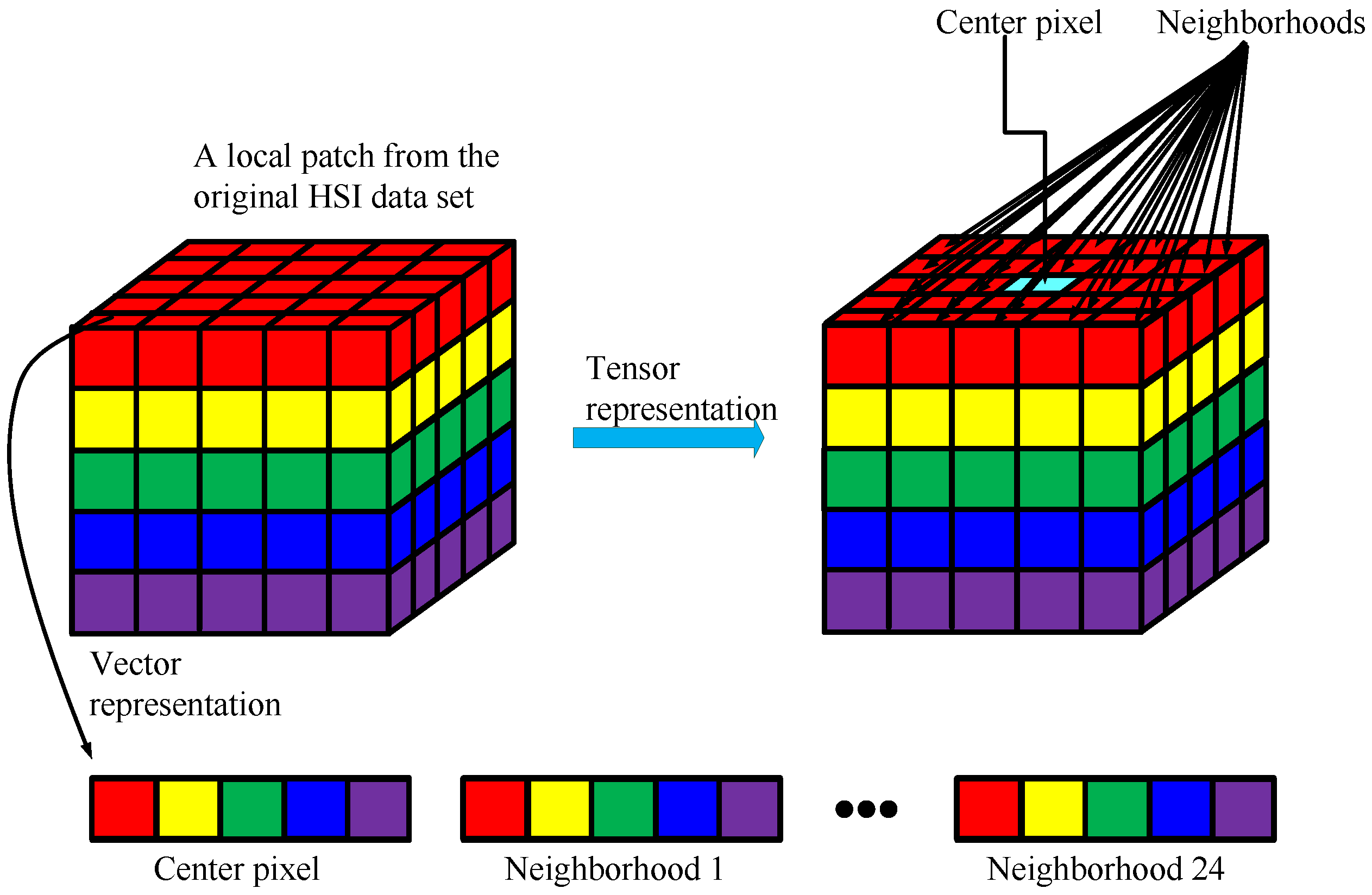
• Spectral-spatial information of pixels is preserved by treating the HSI cube as a third-order tensor. Compared to the vector-based methods, the proposed tensor-based method is capable of maintaining the structural information.
• Proper dictionaries are provided by tensor block-sparsity based learning. Instead of using all of the training samples to construct the dictionaries, the proposed method detects class-discriminative information for classification.
• Class label information is fully exploited by class-dependent block sparse representation. The proposed method learns the sparse coefficients by taking advantage of the class labels, while in general SRC methods, the label information is only used to calculate the residuals.

The layout of this paper is as follows. Section 2 briefly describes the tensor notations and preliminaries. Section 3 illustrates the basic principles of SRC. Section 4 presents the proposed tensor block-sparsity based representation method in detail. Experimental results of two benchmark HSIs are reported in Section 5. Finally, conclusions are drawn in Section 6.

2. Tensor Notations and Preliminaries

A tensor of order N (i.e., a N-dimensional data array) can be expressed by an underlined boldface capital letter, e.g., $\underline{\mathit{A}}\in {\mathbb{R}}^{I_1\times I_2\times \dots \times I_N}$. A matrix (i.e., two-dimensional (2-D) array) is denoted by a boldface uppercase letter and a vector by a boldface lowercase letter, e.g., $\mathit{A}\in {\mathbb{R}}^{I_1\times I_2}$ and $\mathit{a}\in {\mathbb{R}}^I$ represent a matrix and a vector, respectively. The element $(i_1,i_2,\dots ,i_N)$ of a tensor $\underline{\mathit{A}}$ is expressed as $a_{i_1,i_2,\dots ,i_N}$, where $1\le i_n\le I_n$. The Frobenius norm of a tensor $\underline{\mathit{A}}$ is defined as $\parallel \underline{\mathit{A}}{\parallel }_F=\sqrt{{\sum }_{i_1,i_2,\dots ,i_N}{\left|a_{i_1\dots i_N}\right|}^2}$.

A sub-tensor can be formed by restricting the indices to a certain subset of values. This means that given a tensor $\underline{\mathit{A}}\in {\mathbb{R}}^{I_1\times I_2\times \dots \times I_N}$, its mode-n fiber is a vector defined by fixing all indices except $i_n$. Mode-n unfolding (i.e., mode-n matricization) of a tensor $\underline{\mathit{A}}$ yields a matrix ${\mathit{A}}_{\left(n\right)}\in {\mathbb{R}}^{I_n\times {\overline{I}}_n}({\overline{I}}_n={\prod }_{m\ne n}{I}_m)$, whose columns are composed of the mode-n fibers of $\underline{\mathit{A}}$, i.e., ${\mathit{A}}_{\left(1\right)}\in {\mathbb{R}}^{I_1\times I_2{I}_3\dots I_N}$, ${\mathit{A}}_{\left(2\right)}\in {\mathbb{R}}^{I_2\times I_1{I}_3\dots I_N}$, etc. The n-rank of $\underline{\mathit{A}}$, referred to as $r_n$, is defined by the rank of the mode-n unfolding matrix, i.e., $r_n=\mathrm{rank}\left({\mathit{A}}_{\left(n\right)}\right)$.

The product between two matrices can be extended to the product of a tensor and a matrix. Given a tensor $\underline{\mathit{A}}\in {\mathbb{R}}^{I_1\times I_2\times \dots \times I_N}$ and a matrix $\mathit{B}\in {\mathbb{R}}^{J\times I_n}$, the mode-n tensor by matrix product yields $\underline{\mathit{C}}=\underline{\mathit{A}}{\times }_n\mathit{B}\in {\mathbb{R}}^{I_1\times I_2\dots I_{n-1}\times J\times I_{n+1}\dots I_N}$, whose entries are modeled by

$${\displaystyle c_{i_1{i}_2\dots i_{n-1}j{i}_{n+1}\dots i_N}=\sum _{i_n=1}^{I_n}{a}_{i_1{i}_2\dots i_{n-1}{i}_n{i}_{n+1}\dots i_N}{b}_{j{i}_n}}$$

(1)

with $i_k=1,2,\dots ,I_k,(k\ne n)$ and $j=1,2,\dots ,J$. It is worth stressing that the mode-n product $\underline{\mathit{C}}$ corresponds to the product of matrix $\mathit{B}$ by each of the mode-n fibers of $\underline{\mathit{A}}$ because ${\mathit{C}}_{\left(n\right)}=\mathit{B}{\mathit{A}}_{\left(n\right)}$.

The Kronecker product of two matrices, denoted by “⊗”, is an important mathematical operation utilized in this paper. Given two matrices $\tilde{\mathit{A}}\in {\mathbb{R}}^{I_1\times I_2}$ and $\tilde{\mathit{B}}\in {\mathbb{R}}^{I_3\times I_4}$, the Kronecker product $\tilde{\mathit{A}}\otimes \tilde{\mathit{B}}$ is defined as

$$\tilde{\mathit{A}}\otimes \tilde{\mathit{B}}=\left[\begin{array}{cccc}{\tilde{a}}_{11}\tilde{\mathit{B}}& {\tilde{a}}_{12}\tilde{\mathit{B}}& \cdots & {\tilde{a}}_{1I_2}\tilde{\mathit{B}}\\ {\tilde{a}}_{21}\tilde{\mathit{B}}& {\tilde{a}}_{22}\tilde{\mathit{B}}& \cdots & {\tilde{a}}_{2I_2}\tilde{\mathit{B}}\\ ⋮& ⋮& \ddots & ⋮\\ {\tilde{a}}_{I_{1}1}\tilde{\mathit{B}}& {\tilde{a}}_{I_{1}2}\tilde{\mathit{B}}& \cdots & {\tilde{a}}_{I_1{I}_2}\tilde{\mathit{B}}\end{array}\right]\in {\mathbb{R}}^{I_1{I}_3\times I_2{I}_4}$$

(2)

With respect to HSI, it can be regarded as a 3-D data array $\underline{\mathit{A}}\in {\mathbb{R}}^{L_w\times L_h\times l_s}$, where $L_w,L_h$ and $l_s$ indicate the number of rows, columns and spectral bands, respectively. In merit of the tensor algebra, one can perform spectral-spatial classification by treating the HSI as a whole entity. Interested readers can consult [39,41,49,50,51] for more details. Moreover, as shown in Figure 1, the original spatial structure is preserved by tensor, while the spatially connected constraint among local neighborhoods is lost in the vector representation. That means, rather than neglecting the 3-D structure of HSI, information from the spatial domain is implicitly exploited by tensors in the proposed method.

3. Sparse Representation Classifier

SRC is a compressed sensing-inspired technique that has recently been developed as a powerful tool in HSI classification. Relying on the assumption that hyperspectral pixels of the same class generally belong to the same low-dimensional subspace, an unknown test sample $\mathit{x}\in {\mathbb{R}}^{l_s}$ can be represented as a sparse linear combination of all of the training samples

$$\mathit{x}=\mathit{Dz}$$

(3)

where $\mathit{D}=\left[\begin{array}{cccc}{\mathit{d}}_1& {\mathit{d}}_2& \dots & {\mathit{d}}_N\end{array}\right]\in {\mathbb{R}}^{l_s\times N}$ is a structured dictionary formed from the N training samples ${\left\{{\mathit{d}}_i\right\}}_{i=1,2,\dots ,N}$ of all classes, N is the number of training samples from c classes, $l_s$ denotes the number of spectral bands, and $\mathit{z}\in {\mathbb{R}}^N$ indicates an unknown sparse coefficient vector, which can be determined by solving the following optimization problem

$$\widehat{\mathit{z}}=\arg \min {∥\mathit{z}∥}_0\mathrm{s}.\mathrm{t}.\mathit{x}=\mathit{D}\mathit{z}$$

(4)

where the $l_0$-norm ${\parallel ·\parallel }_0$ refers to the number of non-zero entries in $\mathit{z}$. Problem (4) is nondeterministic polynomial-time hard (NP-hard), which cannot be solved in polynomial time. Fortunately, it can be approximately solved by greedy algorithm, such as orthogonal matching pursuit (OMP) [52]. Moreover, the $l_0$-norm problem can also be replaced with an $l_1$-norm problem and be approximately solved by basis pursuit (BP) [53].

Having evaluated $\widehat{\mathit{z}}$, the class label of the test sample $\mathit{x}$ is determined by the minimal error between $\mathit{x}$ and its sub-dictionary estimations

$$\mathrm{class}\mathit{x}=\arg \underset{k=1,2,\dots ,c}{\min }{∥\mathit{x}-{\mathit{D}}_k{\widehat{\mathit{z}}}_k∥}_2$$

(5)

where ${\mathit{D}}_k$ indicates the sub-dictionary from $\mathit{D}$ belonging to the kth class and ${\widehat{\mathit{z}}}_k$ denotes the collection of coefficients in $\widehat{\mathit{z}}$ belonging to the kth class.

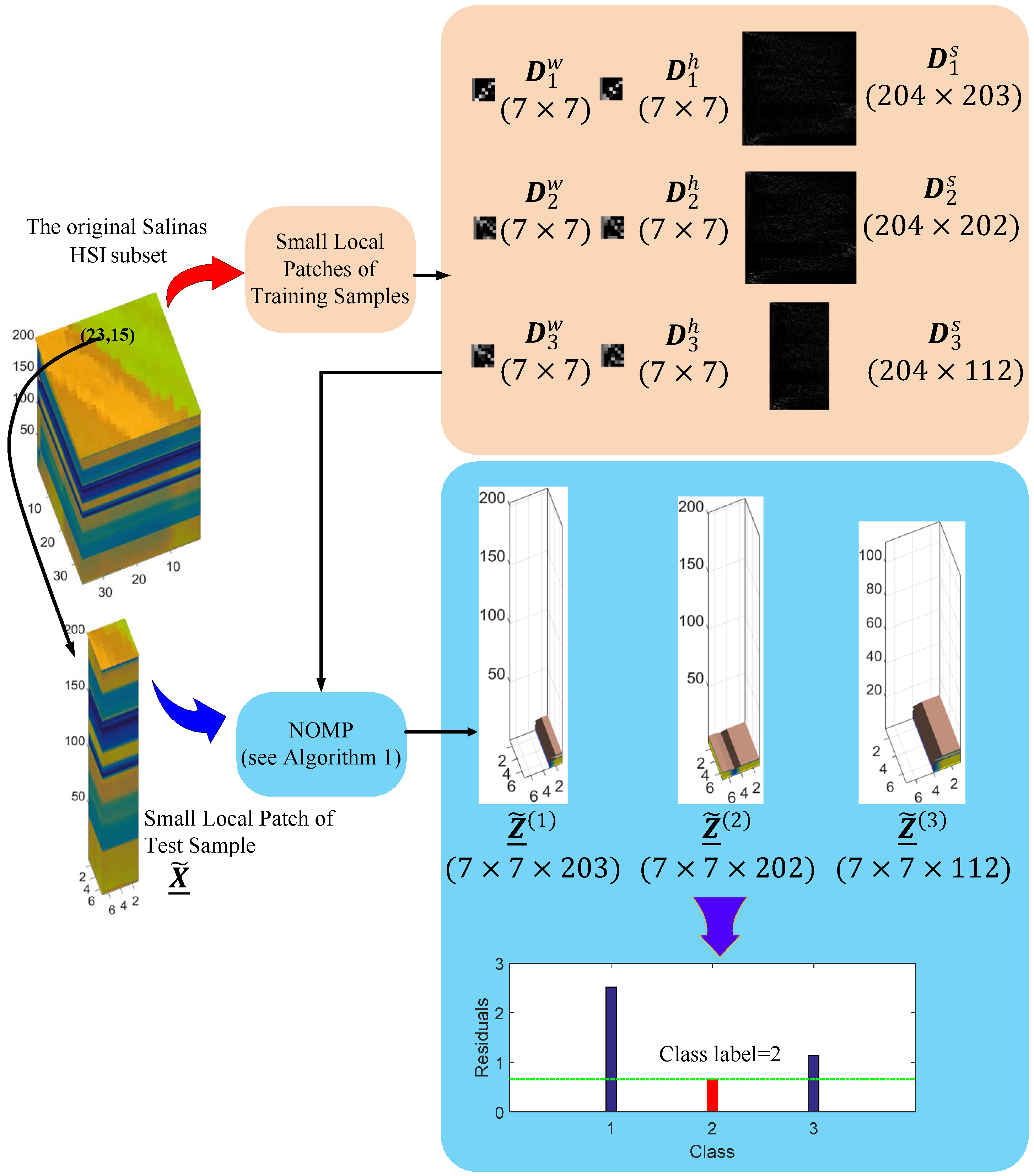
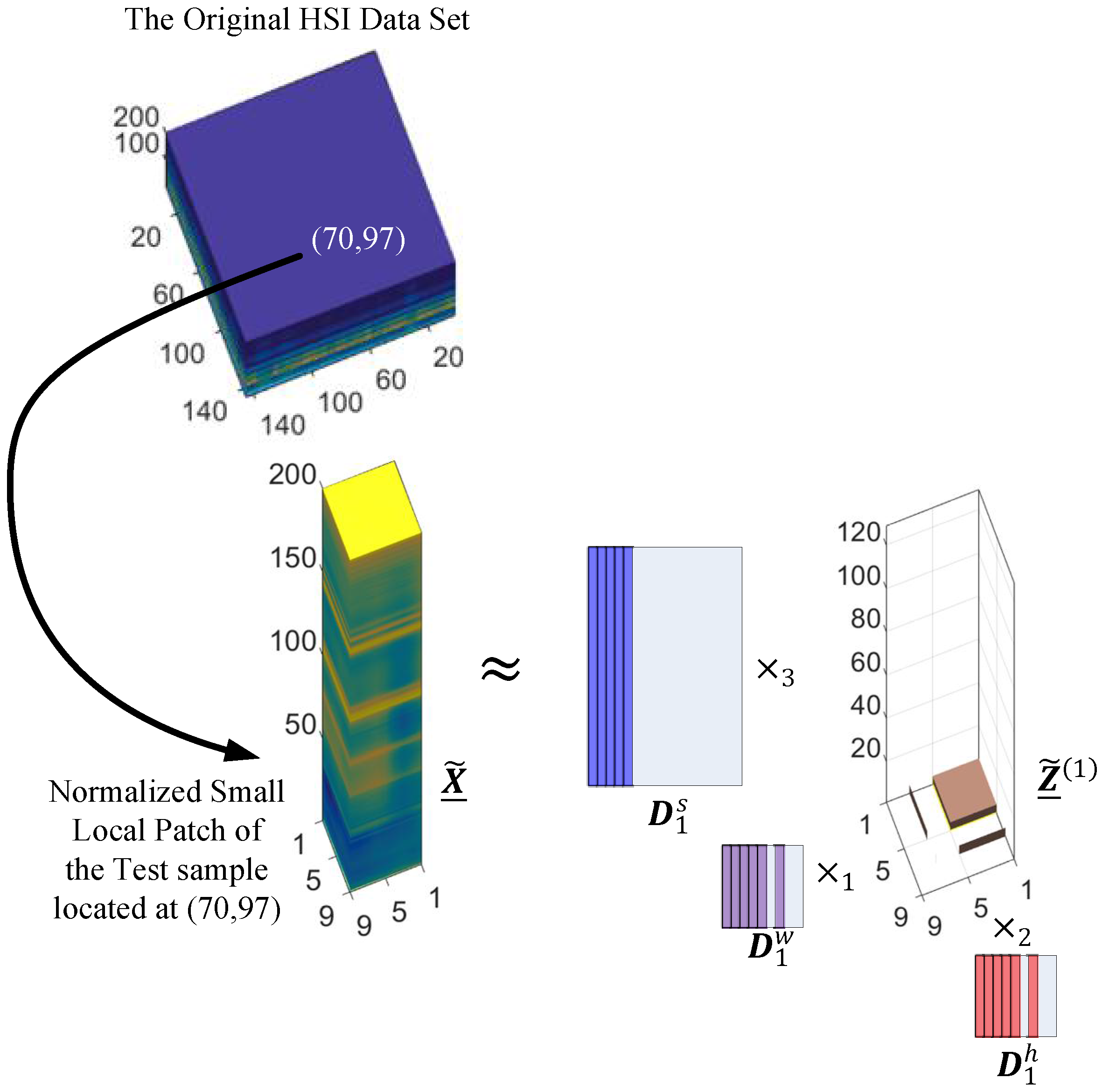
4. Tensor Block-Sparsity based Representation for HSI

Figure 2 depicts the schematic diagram of the proposed tensor block-sparsity based representation method, which consists of two main components. The first one is the tensor block-sparsity based dictionary learning. In this step, a number of small patches are extracted from the original HSI. Each patch is a third-order tensor consisting of a training sample located at the center of the patch and several spatial neighborhoods of the training sample. The patches are then partitioned into c groups. As shown in Figure 2, we categorize the patches into the same group in case the training samples in those patches belong to the same class. Accordingly, the dictionaries can be learned on the c groups with a tensor block-sparsity constraint. The second step is class-dependent block sparse representation. Similar to the training samples, a test sample is expressed as a small local patch with several neighboring pixels surrounding it. The sparse coding of the test sample is then obtained by performing block sparse representation in a class-wise manner. The class label is finally determined by the minimal residual between the test sample and its approximation.

The two above-mentioned steps in the proposed method naturally treat the 3-D HSI data as a third-order tensor to perform the tensor-based dictionary learning and sparse representation. In this regard, the spectral and spatial information can be simultaneously preserved. Moreover, the class-dependent dictionaries generated in the first step help to implement the block sparse representation in a class-wise manner. Note that the traditional SRC ignores the class label information in sparse coding, the classification performance of the proposed method can be improved by taking full advantage of the class labels.

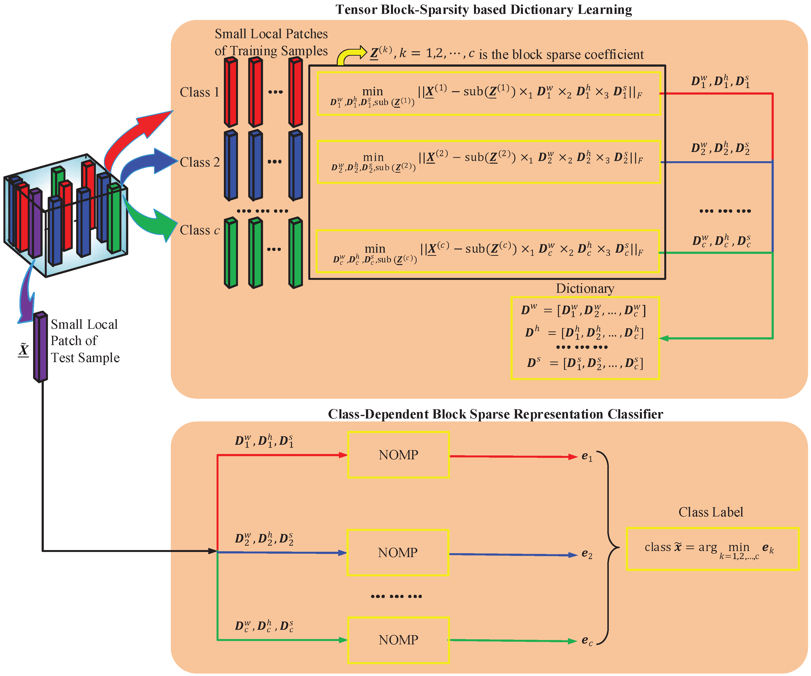
4.1. Tensor Block-Sparsity Based Dictionary Learning

In this paper, the HSI cube is modeled as a third-order tensor $\underline{\mathit{H}}\in {\mathbb{R}}^{L_w\times L_h\times l_s}$, and a small patch is composed of a training sample and its corresponding $l_w\times l_h$ spatial neighborhoods. Suppose ${\underline{\mathit{X}}}_{k,j}\in {\mathbb{R}}^{l_w\times l_h\times l_s}$ denotes the jth patch in the kth group, where $l_w$ and $l_h$ refer to the width and height of the patch, respectively, $l_s$ represents the number of spectral bands, j denotes the index of patch, and $k=1,2,\dots ,c$ corresponds to the index of a group. We then express ${\left\{{\underline{\mathit{X}}}_{k,j}\right\}}_{j=1}^{n_k}$ as the kth group connected to the patches belonging to the kth class, where $n_k$ represents the number of patches in the kth group. For notational convenience, patches of the kth group ${\left\{{\underline{\mathit{X}}}_{k,j}\right\}}_{j=1}^{n_k}$ are combined together to generate a fourth-order tensor ${\underline{\mathit{X}}}^{\left(k\right)}\in {\mathbb{R}}^{l_w\times l_h\times l_s\times n_k}$, whose fourth order mode demonstrates the patches of the kth class.

With ${\underline{\mathit{X}}}^{\left(k\right)},k=1,2,\dots ,c$, the optimization problem for dictionary learning can be modeled as

$$\begin{array}{ccc}\hfill \underset{{\mathit{D}}^w,{\mathit{D}}^h,{\mathit{D}}^s,{\underline{\mathit{Z}}}^{\left(k\right)}}{\min }& & {\displaystyle \sum _{k=1}^c{\parallel {\underline{\mathit{X}}}^{\left(k\right)}-{\underline{\mathit{Z}}}^{\left(k\right)}{\times }_1{\mathit{D}}^w{\times }_2{\mathit{D}}^h{\times }_3{\mathit{D}}^s\parallel }_F}\hfill \\ \hfill \mathrm{s}.\mathrm{t}.& & \parallel {\underline{\mathit{Z}}}^{\left(k\right)}{\parallel }_B⪯(r_k^w,r_k^h,r_k^s),k=1,2,\dots ,c\hfill \end{array}$$

(6)

where ${\mathit{D}}^w\in {\mathbb{R}}^{l_w\times m_w}$, ${\mathit{D}}^h\in {\mathbb{R}}^{l_h\times m_h}$, ${\mathit{D}}^s\in {\mathbb{R}}^{l_s\times m_s}$ are the dictionaries to be learned, $m_w={\sum }_{k=1}^c{r}_k^w$, $m_h={\sum }_{k=1}^c{r}_k^h$, $m_s={\sum }_{k=1}^c{r}_k^s$, $r_k^w$, $r_k^h$ and $r_k^s$ are the tensor block-sparsity parameters, the “tensor block-sparsity” of ${\underline{\mathit{Z}}}^{\left(k\right)}$ is equal to ($r_k^w,r_k^h,r_k^s$) if and only if the indices ${\mathit{I}}^w,{\mathit{I}}^h,{\mathit{I}}^s$ which satisfy $z_{i_1{i}_2{i}_3{i}_4}^{\left(k\right)}=0$ for all $(i_1,i_2,i_3)\notin {\mathit{I}}^w\times {\mathit{I}}^h\times {\mathit{I}}^s$ contain at least $r_k^w,r_k^h,r_k^s$ elements, ${\mathit{a}}_1⪯{\mathit{a}}_2$ implies that each entry of ${\mathit{a}}_1$ is not greater than the corresponding entry of ${\mathit{a}}_2$, ${\parallel ·\parallel }_F$ denotes Frobenius norm, i.e., the square root of the sum of the absolute squares of the elements, ${\underline{\mathit{Z}}}^{\left(k\right)}\in {\mathbb{R}}^{m_w\times m_h\times m_s\times n_k}$, and $\parallel {\underline{\mathit{Z}}}^{\left(k\right)}{\parallel }_B$ represents the “tensor block-sparsity” of ${\underline{\mathit{Z}}}^{\left(k\right)}$.

Note that the dictionary learning problem in Equation (6) can be decoupled into c sub-problems. As such, the dictionary learning can be performed independently for each class to yield class-dependent dictionaries, which helps to achieve class-dependent block sparse representation. Specifically, the kth element in the objective function of Equation (6) can be formulated as

$$\begin{array}{cc}& \parallel {\underline{\mathit{X}}}^{\left(k\right)}-{\underline{\mathit{Z}}}^{\left(k\right)}{\times }_1{\mathit{D}}^w{\times }_2{\mathit{D}}^h{\times }_3{\mathit{D}}^s{\parallel }_F\hfill \\ =& \parallel {\underline{\mathit{X}}}^{\left(k\right)}-\mathrm{sub}\left({\underline{\mathit{Z}}}^{\left(k\right)}\right){\times }_1{\mathit{D}}_k^w{\times }_2{\mathit{D}}_k^h{\times }_3{\mathit{D}}_k^s{\parallel }_F\hfill \end{array}$$

(7)

where $\mathrm{sub}\left({\underline{\mathit{Z}}}^{\left(k\right)}\right)\in {\mathbb{R}}^{r_k^w\times r_k^h\times r_k^s\times n_k}$ represents the support set of ${\underline{\mathit{Z}}}^{\left(k\right)}$, ${\mathit{D}}^w=[{\mathit{D}}_1^w,{\mathit{D}}_2^w,\dots ,{\mathit{D}}_c^w]$, ${\mathit{D}}^h=[{\mathit{D}}_1^h,{\mathit{D}}_2^h,\dots ,{\mathit{D}}_c^h]$ and ${\mathit{D}}^s=[{\mathit{D}}_1^s,{\mathit{D}}_2^s,\dots ,{\mathit{D}}_c^s]$.

Let $\underline{\mathit{Y}}=\mathrm{sub}\left({\underline{\mathit{Z}}}^{\left(k\right)}\right)$, the tensor block-sparsity constraints of Equation (6) are implicitly satisfied by setting $\underline{\mathit{Y}}\in {\mathbb{R}}^{r_k^w\times r_k^h\times r_k^s\times n_k}$. In this regard, the original dictionary learning model in Equation (6) can be divided into a number of unconstrained problems imposed on the c groups

$$\begin{array}{cc}\hfill \underset{{\mathit{D}}_k^w,{\mathit{D}}_k^h,{\mathit{D}}_k^s,\underline{\mathit{Y}}}{\min }& \parallel {\underline{\mathit{X}}}^{\left(k\right)}-\underline{\mathit{Y}}{\times }_1{\mathit{D}}_k^w{\times }_2{\mathit{D}}_k^h{\times }_3{\mathit{D}}_k^s{\parallel }_F\end{array}$$

(8)

Moreover, Equation (8) can be equivalently represented as

$$\begin{array}{cc}\hfill \underset{{\mathit{U}}_1,{\mathit{U}}_2,{\mathit{U}}_3,{\mathit{U}}_4,\underline{\mathit{G}}}{\min }& \parallel {\underline{\mathit{X}}}^{\left(k\right)}-\underline{\mathit{G}}{\times }_1{\mathit{U}}_1{\times }_2{\mathit{U}}_2{\times }_3{\mathit{U}}_3{\times }_4{\mathit{U}}_4{\parallel }_F\end{array}$$

(9)

where $\underline{\mathit{G}}\in {\mathbb{R}}^{r_k^w\times r_k^h\times r_k^s\times r_k^n}$ denotes the core tensor and ${\mathit{U}}_1\in {\mathbb{R}}^{l_k^w\times r_k^w}$, ${\mathit{U}}_2\in {\mathbb{R}}^{l_k^h\times r_k^h}$, ${\mathit{U}}_3\in {\mathbb{R}}^{l_k^s\times r_k^s}$, ${\mathit{U}}_4\in {\mathbb{R}}^{n_k\times r_k^n}$ contain the basis vectors in the four modes of $\underline{\mathit{X}}$.

The tensor block-sparsity parameters $r_k^w,r_k^h,r_k^s$ and $r_k^n$ can be obtained via the minimum description length (MDL) method [54]. Comparing Equations (8) and (9), we observe that ${\mathit{D}}_k^w={\mathit{U}}_1$, ${\mathit{D}}_k^h={\mathit{U}}_2$, ${\mathit{D}}_k^s={\mathit{U}}_3$ and $\underline{\mathit{Y}}=\underline{\mathit{G}}{\times }_4{\mathit{U}}_4$. Since the problem of Equation (9) can be effectively solved by the Tucker decomposition (http://www.sandia.gov/∼tgkolda/TensorToolbox/index-2.6.html) [55], the solution of Equation (8) is also determined accordingly.

4.2. Class-Dependent Block Sparse Representation Classifier

Analogous to the training samples, a test sample $\tilde{\mathit{x}}\in {\mathbb{R}}^{l_s}$ can also be extended to a third-order tensor $\widetilde{\underline{\mathit{X}}}\in {\mathbb{R}}^{l_w\times l_h\times l_s}$ by utilizing the $l_w\times l_h$ spatial neighboring pixels of $\tilde{\mathit{x}}$. Notice that the traditional SRC only incorporates the class label information when identifying the reconstruction errors (see Equation (5)), which is generally not included in the learning stage (see Equation (4)). To fully exploit the class label information in the learning process, we propose a class-dependent block sparse representation classifier. The idea is to successively represent $\widetilde{\underline{\mathit{X}}}$ by the kth $(k=1,2,\dots ,c)$ group dictionaries $({\mathit{D}}_k^w,{\mathit{D}}_k^h,{\mathit{D}}_k^s)$ and constrain block-structured sparsity on the core tensor ${\widetilde{\underline{\mathit{Z}}}}^{\left(k\right)}$. This means that the sparse coding is obtained by solving

$$\begin{array}{ccc}\hfill \underset{{\widetilde{\underline{\mathit{Z}}}}^{\left(k\right)}}{\min }& & \parallel \widetilde{\underline{\mathit{X}}}-{\widetilde{\underline{\mathit{Z}}}}^{\left(k\right)}{\times }_1{\mathit{D}}_k^w{\times }_2{\mathit{D}}_k^h{\times }_3{\mathit{D}}_k^s{\parallel }_F\hfill \\ \hfill \mathrm{s}.\mathrm{t}.& & \parallel {\widetilde{\underline{\mathit{Z}}}}^{\left(k\right)}{\parallel }_B⪯({\tilde{r}}_k^w,{\tilde{r}}_k^h,{\tilde{r}}_k^s)\hfill \end{array}$$

(10)

The constraint of Equation (10) restricts the non-zero entries of the core tensor ${\widetilde{\underline{\mathit{Z}}}}^{\left(k\right)}$ to be located in a sub-tensor with size ${\tilde{r}}_k^w\times {\tilde{r}}_k^h\times {\tilde{r}}_k^s$. The main advantage of sparse coding is that it can improve the discrimination of the classifier. That is because, suppose the test sample $\tilde{\mathit{x}}$ belong to class i, it is more probable to represent $\widetilde{\underline{\mathit{X}}}$ by a few atoms from $({\mathit{D}}_i^w,{\mathit{D}}_i^h,{\mathit{D}}_i^s)$ with a satisfactory accuracy, while more atoms from other classes (e.g., $({\mathit{D}}_j^w,{\mathit{D}}_j^h,{\mathit{D}}_j^s)$) are needed to represent $\widetilde{\underline{\mathit{X}}}$ with the same accuracy. Therefore, the representation error of $\widetilde{\underline{\mathit{X}}}$ by $({\mathit{D}}_i^w,{\mathit{D}}_i^h,{\mathit{D}}_i^s)$ will be smaller than other classes under a certain sparsity constraint. Moreover, we visually illustrate the unstructured and block sparsity of ${\widetilde{\underline{\mathit{Z}}}}^{\left(k\right)}$ in Figure 3, from which one can observe that the structured information is effectively incorporated into the block-sparsity-based method whereas no such information is contained in the unstructured-based method. It is notable that the additional assumption about the location of nonzero sparse coefficients (i.e., “structured sparsity”) facilitates the reduction of complexity in solving Equation (10).

In this paper, we adopt the N-way block OMP (NOMP) to solve Equation (10). The NOMP is a greedy algorithm proposed by Caiafa et al. [47,48]. As a tensor extension of the traditional one-dimensional (1-D) OMP, NOMP iteratively selects the dictionary element correlated with the current residuals and is computationally efficient due to the full use of the sparsity structure under the tensor block-sparsity assumption. A detailed classification process is illustrated in Algorithm 1, in which steps 3–10 aim at identifying the core tensor ${\widetilde{\underline{\mathit{Z}}}}^{\left(k\right)}$ and the residual ${\mathit{e}}_k$. Analogous to SRC, the class label of $\tilde{\mathit{x}}$ is determined by the minimal residual

$$\mathrm{class}\tilde{\mathit{x}}=\arg \underset{k=1,2,\dots ,c}{\min }{\mathit{e}}_k$$

(11)

where

$${\mathit{e}}_k={∥vec\left(\widetilde{\underline{\mathit{X}}}-{\widetilde{\underline{\mathit{Z}}}}^{\left(k\right)}({\mathcal{I}}_1^{\left(k\right)},{\mathcal{I}}_2^{\left(k\right)},{\mathcal{I}}_3^{\left(k\right)}){\times }_1{\mathit{D}}_k^w(:,{\mathcal{I}}_1^{\left(k\right)}){\times }_2{\mathit{D}}_k^h(:,{\mathcal{I}}_2^{\left(k\right)}){\times }_3{\mathit{D}}_k^s(:,{\mathcal{I}}_3^{\left(k\right)})\right)∥}_2$$

(12)

$vec(·)$ denotes the vectorization operator and ${\mathcal{I}}_1^{\left(k\right)},{\mathcal{I}}_2^{\left(k\right)}$ and ${\mathcal{I}}_3^{\left(k\right)}$ are the support sets of ${\widetilde{\underline{\mathit{Z}}}}^{\left(k\right)}$.

Algorithm 1: Class-Dependent Block Sparse Representation Classifier
Require: Dictionaries $({\mathit{D}}_k^w,{\mathit{D}}_k^h,{\mathit{D}}_k^s)$, $k=1,2,\dots ,c$, sparsity level S, test sample $\tilde{\mathit{x}}$ and its corresponding third-order tensor $\widetilde{\underline{\mathit{X}}}$ composed of the neighboring pixels
Ensure: The class label of test sample $\tilde{\mathit{x}}$
1:	for all $k=1,2,\dots ,c$ do
2:	Set $m=1$, ${\mathcal{I}}_1^{\left(k\right)},{\mathcal{I}}_2^{\left(k\right)},{\mathcal{I}}_3^{\left(k\right)}=⌀$, ${\widetilde{\underline{\mathit{Z}}}}^{\left(k\right)}=\underline{\mathbf{0}}$ and ${\underline{\mathit{R}}}_k^m=\widetilde{\underline{\mathit{X}}}$
3:	while $m\le S$ do
4:	$(i_1^{\left(m\right)},i_2^{\left(m\right)},i_3^{\left(m\right)})=\arg \underset{i_1,i_2,i_3}{\max }\left|\underline{\mathit{R}}{\times }_1{\mathit{D}}_k^w{(:,i_1)}^{\mathrm{T}}{\times }_2{\mathit{D}}_k^h{(:,i_2)}^{\mathrm{T}}{\times }_3{\mathit{D}}_k^s{(:,i_3)}^{\mathrm{T}}\right|$
5:	Update the support set ${\mathcal{I}}_1^{\left(k\right)}={\mathcal{I}}_1^{\left(k\right)}\cup i_1^{\left(m\right)}$, ${\mathcal{I}}_2^{\left(k\right)}={\mathcal{I}}_2^{\left(k\right)}\cup i_2^{\left(m\right)}$, ${\mathcal{I}}_3^{\left(k\right)}={\mathcal{I}}_3^{\left(k\right)}\cup i_3^{\left(m\right)}$
6:	Identify the vectorized version of ${\widetilde{\underline{\mathit{Z}}}}^{\left(k\right)}$ by
	${\tilde{\mathit{z}}}^{\left(k\right)}=\arg \underset{\tilde{\mathit{z}}}{\min }{∥\left({\mathit{D}}_k^s(:,{\mathcal{I}}_3^{\left(k\right)})\otimes {\mathit{D}}_k^h(:,{\mathcal{I}}_2^{\left(k\right)})\otimes {\mathit{D}}_k^w(:,{\mathcal{I}}_1^{\left(k\right)})\right)\tilde{\mathit{z}}-\tilde{\mathit{x}}∥}_2$
7:	Compute the residual ${\underline{\mathit{E}}}_k^m=\widetilde{\underline{\mathit{X}}}-{\widetilde{\underline{\mathit{Z}}}}^{\left(k\right)}({\mathcal{I}}_1^{\left(k\right)},{\mathcal{I}}_2^{\left(k\right)},{\mathcal{I}}_3^{\left(k\right)}){\times }_1{\mathit{D}}_k^w(:,{\mathcal{I}}_1^{\left(k\right)}){\times }_2{\mathit{D}}_k^h(:,{\mathcal{I}}_2^{\left(k\right)}){\times }_3{\mathit{D}}_k^s(:,{\mathcal{I}}_3^{\left(k\right)})$
8:	$m=m+1$
9:	end while
10:	Calculate the norm of the kth residual ${\mathit{e}}_k={∥{\mathit{e}}_k^{m-1}∥}_2$, where ${\mathit{e}}_k^{m-1}$ is the vectorization of ${\underline{\mathit{E}}}_k^{m-1}$
11:	end for
12:	Determine the class label of $\tilde{\mathit{x}}$ by $\mathrm{class}\tilde{\mathit{x}}=\arg \underset{k=1,2,\dots ,c}{\min }{\mathit{e}}_k$

4.3. A Synthetic Example

Having displayed the tensor block-sparsity based representation method, a synthetic example is provided in this subsection to demonstrate the parameterization, learning and utilization of the spatial information. The HSI data set used in this example is cropped from the whole Salinas-A scene (http://www.ehu.eus/ccwintco/index.php?title=Hyperspectral_Remote_Sensing_Scenes), i.e., columns [1,2,3,4,5,6,7,8,9,10,11,12,13,14,15,16,17,18,19,20,21,22,23,24,25,26,27,28,29,30,31,32,33,34,35,36] and rows [1,2,3,4,5,6,7,8,9,10,11,12,13,14,15,16,17,18,19,20,21,22,23,24,25,26,27,28,29,30,31,32,33,34,35,36] having the size of 36 × 36 × 204 containing 3 classes of interest ($c=3$). 5% of the samples from each class are chosen for training while the rest ones are taken as test samples. Without loss of generality, we demonstrate how to identify the class label of a test sample located at (23, 15) (belong to class 2). As shown in Figure 4, tensor block-sparsity based dictionary learning is first performed on the small local patches (neighborhood size = 7 × 7) of training samples. In this step, spatial information are incorporated in each small 3-D patches. Results of the learned dictionaries $({\mathit{D}}_k^w,{\mathit{D}}_k^h,{\mathit{D}}_k^s)$, $k=1,2,3$ are shown in the top right corner of Figure 4. The size of each dictionary is also displayed. Subsequently, class-dependent block sparse representation is performed on the small local patch of test sample $\widetilde{\underline{\mathit{X}}}\in {\mathbb{R}}^{7\times 7\times 204}$. The core tensors ${\widetilde{\underline{\mathit{Z}}}}^{\left(k\right)},k=1,2,3$ which have obvious structured sparsity is plotted in the lower left corner of Figure 4. Based on the minimal residuals, the class label of the test sample is finally set as 2.

As above analysis, both training and test samples are represented as third-order tensors, which consisted of the training (or test) sample located at the center and several spatial neighborhood. Therefore, rather than neglecting the 3-D structure of HSI, the proposed method maintains spectral-spatial information simultaneously by taking a pixel and its neighborhood as a whole entity.

5. Experimental Section

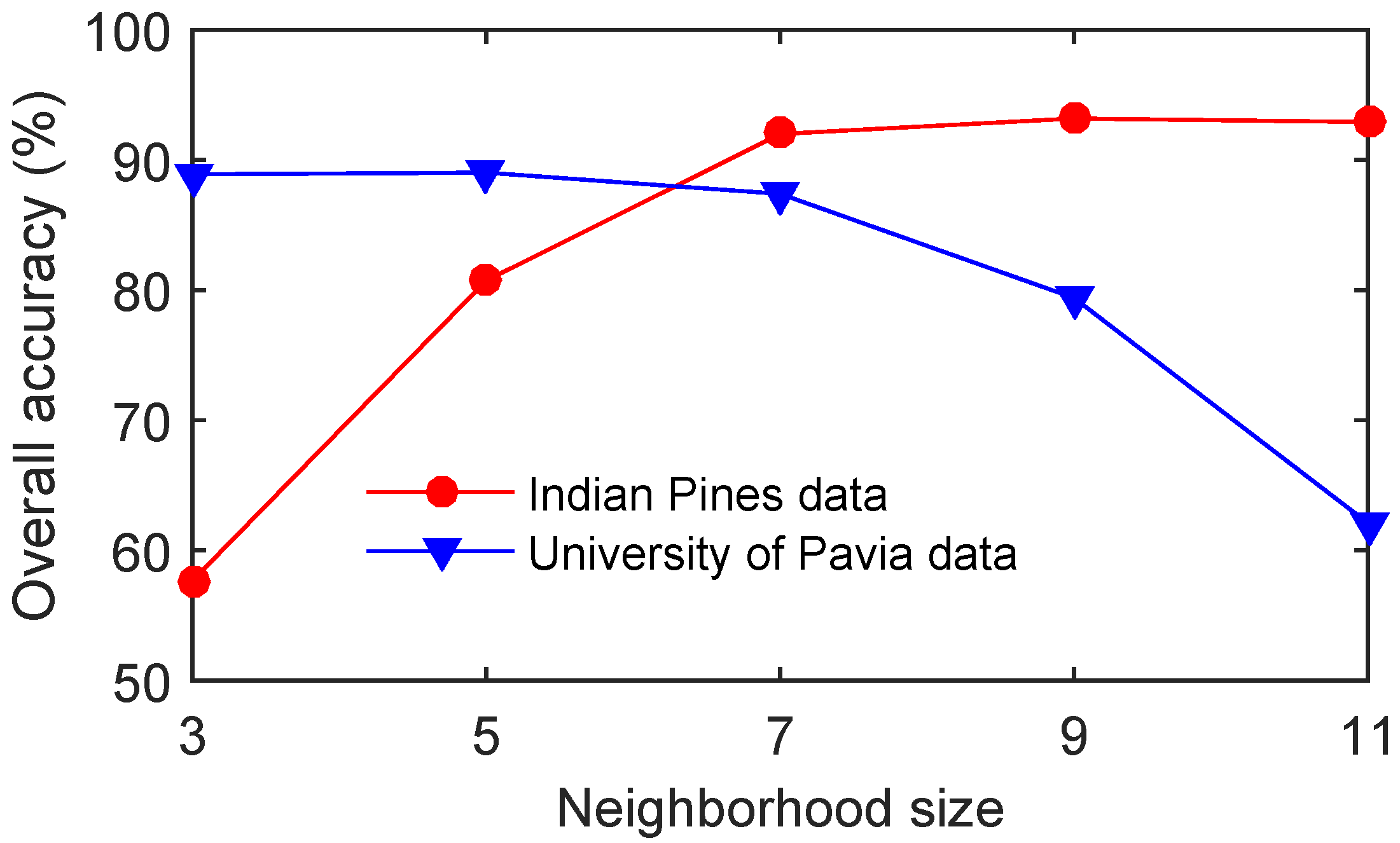
In this section, we perform experiments on two real-world data cubes to assess the effectiveness of the proposed method. The experimental results are compared visually and quantitatively with those gained from several state-of-the-art methods, including the classical SVM [10], the SVM with composite kernel (SVMCK) [19], CRC [33], the JSM solved by simultaneous versions of OMP (denoted by SOMP) [13], SADL [29], 3-D discrete wavelet transform (3D-DWT) [36], LTDA [42], cdSRC [35], and patch-based learning SRC with spatial smooth (pLSRC-S) [32]. Moreover, we abbreviate the proposed tensor block-sparsity based representation classifier as tbSRC for simplicity.

5.1. Data Sets

Two real-world HSI data sets, namely Indian Pines data and University of Pavia data, with various spectral and spatial resolutions reflecting different environments of remote sensing are utilized in the experiments.

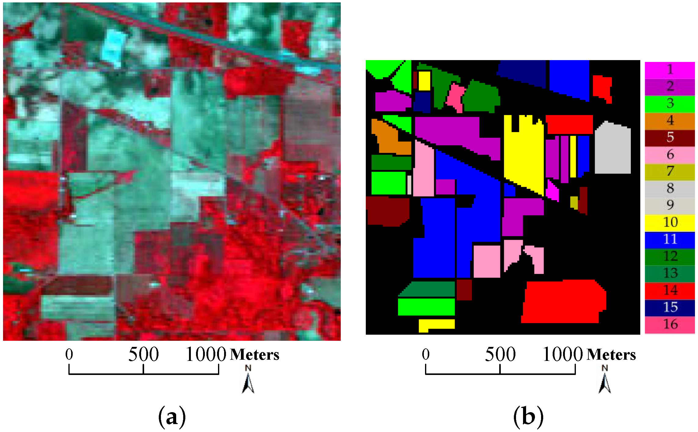
• Indian Pines data: this data set was acquired by the Airborne Visible/Infrared Imaging Spectrometer (AVIRIS) over a mixed forest/agricultural region from Northwestern Indiana in June 1992. The image size is 145 × 145 × 220 ($L_w=145$, $L_h=145$, $l_s=220$) with 145 × 145 pixels and 220 spectral bands. The spatial resolution is 20 m per pixel and the 220 spectral bands cover 0.4–2.5 $\mathsf{\mu }$m range, of which 20 noisy and water-vapor absorption bands (bands 104–108, 150–163, and 220) are removed so that 200 bands are reserved for experiments. Figure 5 displays the three-band false color composite image along with the corresponding ground truth. This data set contains 16 classes of interest and 10366 labeled pixels ranging unbalanced from 20 to 2468, which poses a big challenge for the classification problem. The number of samples for each class is listed in

  Table 1. Number of Samples (No.S) and available training samples (No. ATS) used in the experiments.

  Indian Pines Data				University of Pavia Data
  Class	Name	No.S		Class	Name	No.S	No. ATS
  1	alfalfa	54		1	asphalt	6631	548
  2	corn-no till	1434		2	meadows	18,649	540
  3	corn-min till	834		3	gravel	2099	392
  4	corn	234		4	trees	3064	524
  5	grass/pasture	497		5	metal sheets	1345	265
  6	grass/trees	747		6	bare soil	5029	532
  7	grass/pasture-mowed	26		7	bitumen	1330	375
  8	hay-windrowed	489		8	bricks	3682	514
  9	oats	20		9	shadows	947	231
  10	soybean-no till	968
  11	soybean-min till	2468
  12	soybean-clean till	614
  13	wheat	212
  14	woods	1294
  15	bldg-grass-tree-drives	380
  16	stone-steel towers	95
  Total		10,366		Total		42,776	3921

  , whose background color corresponds to different classes of land covers.
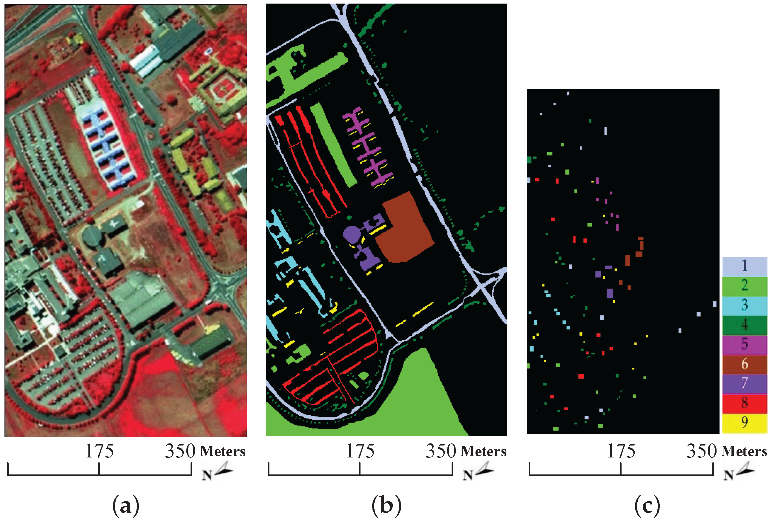
• University of Pavia data: this data set was acquired by the Reflective Optics System Imaging Spectrometer (ROSIS) over the urban site of the University of Pavia, northern Italy, in July 2002. The original size is 610 × 340 × 115 ($L_w=610$, $L_h=340$, $l_s=115$) with 610 × 340 pixels and 115 spectral bands. The spatial resolution is 1.3 m per pixel and the 115 spectral bands cover 0.43–0.86 $\mathsf{\mu }$m, of which the 12 noisiest channels are removed and 103 spectral bands remain for experiments. Figure 6 shows the false color composite image, the ground truth data and the available training samples. Table 1 lists the number of samples for each class together with the available training samples. Analogous to the Indian Pines data, the background color also corresponds to different classes of land covers. As shown in Table 1, this image consists of 9 classes of land covers and each class contains more than 900 pixels. However, the available training samples of each class are less than 600.

5.2. Experimental Design

To demonstrate the performance of the proposed tbSRC, nine widespread methods are considered for comparison:

• SVM: the classical SVM [10] with a single radial basis function (RBF) kernel;
• SVMCK: the SVM [19] with a composite of spectral kernel and spatial kernel, and the spatial feature is extracted by extended morphological profile (EMP) [56];
• CRC: the test sample is approximated by the linear combination of the training samples in a least squares sense [33].
• SOMP: the spectral-spatial SRC incorporating spatial information by JSM and solved by SOMP [13];
• SADL: the spatial-aware classification technique [29] whose dictionary is obtained by structured dictionary learning and sparse coefficients are classified by linear SVM (Different from the SVM, SVMCK, 3D-DWT and LTDA, SADL applies the linear SVM for two reasons: (1) the SADL of this paper is consistent with [29], which employs linear SVM; (2) the sparse codes of SADL are discriminative enough to be well classified by the linear SVM.);
• 3D-DWT: the texture features are obtained by 3D-DWT and the classification results are given by RBF-based SVM [36];
• LTDA: the features are extracted by EMP [56] and LTDA [42] and classified by SVM;
• cdSRC: the SRC for each class is solved by OMP and the class label is jointly determined by the residual and Euclidean distance [35];
• pLSRC-S: the spectral-spatial SRC [32] with spatial smooth and the dictionary is learned by a modified patch-based learning SRC.

Note that: (1) the above-mentioned SVM, CRC and cdSRC are classification methods that use spectral information, while the other ones are spectral-spatial methods; (2) the CRC, SOMP, cdSRC, pLSRC-S and tbSRC are based on collaborative/sparse representation, while the other ones apply SVM for classification; (3) the 3D-DWT, LTDA and tbSRC are tensor-based methods, while the remaining methods ignore the 3-D structure of HSI.

Two experiments are designed in this paper: (1) we perform detailed comparisons on the two data sets with fixed ratios of labeled samples; (2) we also conduct additional comparisons to validate the tbSRC using various small numbers of labeled samples. In experiment 1, approximately 5% of the samples from each class in the Indian Pines data (see the 3rd column of Table 1) are randomly chosen as training samples and the remaining ones as test samples. Since the available training samples are separate from the whole samples in the other two data sets, only 5% of the available training samples (see the last column of Table 1) are randomly selected for training in the University of Pavia data. In experiment 2, we choose 0.5%, 1%, 2%, 3%, 4% and 5% of samples from each class in the Indian Pines data and 0.5%, 1%, 2%, 3%, 4% and 5% of the available training samples in the University of Pavia data as training samples, while the rest are treated as test ones. The aforementioned methods are compared numerically (overall accuracy (OA) and average accuracy (AA)) and statistically (kappa coefficient (κ)). All the experiments demonstrated in this section are implemented with MATLAB on a platform with Intel(R) Xeon(R) CPU (3.3 GHz), 8 GB RAM and a Windows 7 operating system and the results are averaged over 10 independent trials to alleviate possible bias.

Moreover, several parameters should be tuned in the experiments. For the SVM-based methods (i.e., SVM, SVMCK, SADL, 3D-DWT and LTDA), the RBF kernel is used in SVM, SVMCK, 3D-DWT and LTDA, while the linear kernel is adopted in SADL. The RBF parameter γ is tuned in the range $\gamma \in \{2^{-8},2^{-7},\dots ,2^8\}$, the composite weight η in SVMCK is varied in steps of 0.1 in the range 0 to 1, and the penalty term C is set to 60. Figure 7 plots the effect of C ($C\in \{1,2,\dots ,100\}$ with $\gamma =1$) on OA of SVM for the Indian Pines data. As shown in Figure 7, we can find that the parameter C does not seriously affect the classification accuracy of SVM when C is larger than 10. Therefore, we set $C=60$ in the experiments. For the sparse representation-based methods (i.e., SOMP, cdSRC and tbSRC), the sparsity level S ranges from 10 to 100, and the neighborhood of both SOMP and tbSRC ranges from $3\times 3$ to $11\times 11$. Figure 8 shows the optimal OA of various neighborhood sizes in the two HSI data sets. It can be observed that the $9\times 9$ neighborhood yields high accuracy for the Indian Pines data, while smaller sizes are more suitable for the University of Pavia data which lacks large spatial homogeneity. According to [29], the patch size of SADL is taken as $8\times 8$ for the Indian Pines data and $16\times 16$ for the University of Pavia data. The neighborhood size of pLSRC-S [32] is set as $7\times 7$ for the Indian Pines data and $21\times 21$ for the remaining two data sets. Although different methods take different patch sizes, it still makes sense to compare those methods. On the one hand, although a larger patch size is somewhat similar to using more samples, the number of training and test samples used in different methods are the same as each other. On the other hand, the patch size of each patch-based method is set to have the best (or at least comparable) performance, and it is reasonable to compare all of the patch-based methods under their best (or at least comparable) situations. Moreover, the HSI is decomposed into 2 levels in the 3D-DWT, and the dimension is reduced to 30 in the local Fisher discriminant analysis (LFDA) step of cdSRC. In LTDA, 5 and 2 principle components are reserved to obtain the EMP features in the two data sets, respectively.

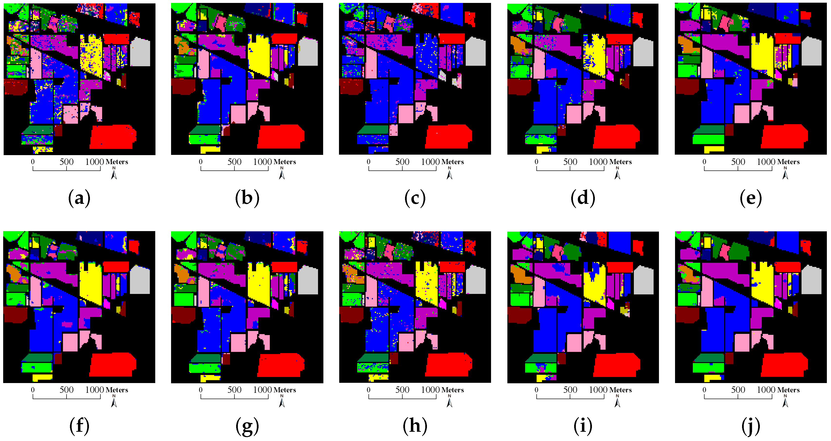
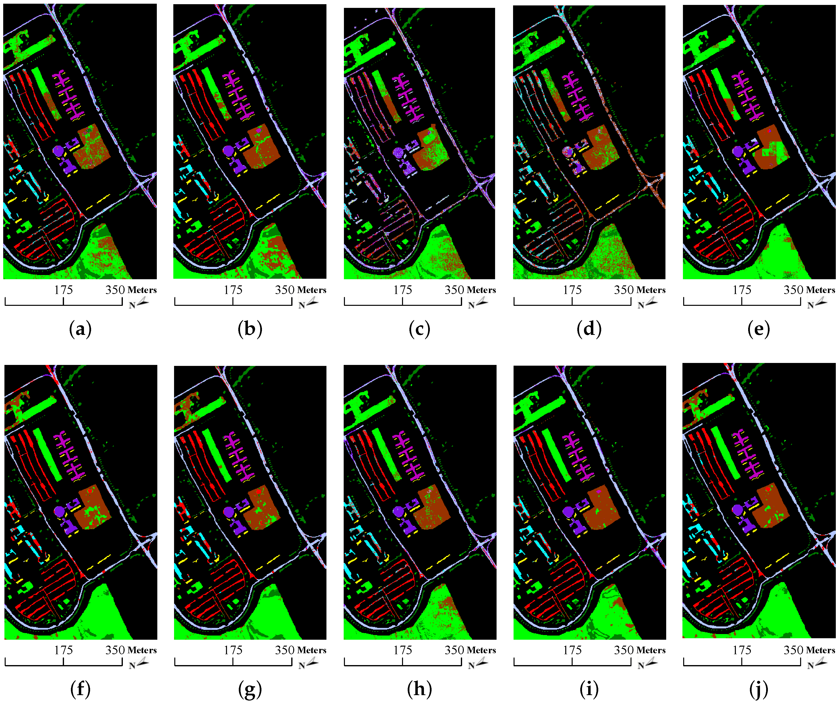
5.3. Classification Results and Discussions of Experiment 1

We first illustrate the block-structured sparsity derived from the real-world Indian Pines data set. Without loss of generality, we choose the test sample (belonging to class 1 alfalfa) from the spatial coordinate $(70,97)$ and let the neighborhood size be $9\times 9$ and $k=1$. As plotted in Figure 9, the normalized small local patch $\widetilde{\underline{\mathit{X}}}\in {\mathbb{R}}^{9\times 9\times 200}$, which comprises the test sample and its $9\times 9$ neighboring pixels, can be approximated by the 1st group dictionaries $({\mathit{D}}_1^w,{\mathit{D}}_1^h,{\mathit{D}}_1^s)$ and the core tensor ${\widetilde{\underline{\mathit{Z}}}}^{\left(1\right)}$ with ${\mathit{D}}_1^w,{\mathit{D}}_1^h\in {\mathbb{R}}^{9\times 9}$, ${\mathit{D}}_1^s\in {\mathbb{R}}^{200\times 129}$, and ${\widetilde{\underline{\mathit{Z}}}}^{\left(1\right)}\in {\mathbb{R}}^{9\times 9\times 129}$. It is observed from Figure 9 that the non-zero elements of ${\widetilde{\underline{\mathit{Z}}}}^{\left(1\right)}$ are concentrated in a few locations and exhibit block structure, which is consistent with the ideal situation shown in Figure 3b.

In the first experiment, different approaches are compared in

Table 2. Classification accuracy (%) and standard deviation (in bracket) of different methods for the Indian Pines data.

Class	SVM	SVMCK	CRC	SOMP	SADL	3D-DWT	LTDA	cdSRC	pLSRC	tbSRC
1	41.18	64.71	0	77.12	76.47	80.39	81.05	88.24	89.41	98.04
2	72.98	83.70	67.11	91.09	90.49	88.03	84.90	86.12	91.42	88.91
3	55.43	85.98	9.57	80.72	92.05	89.90	91.58	81.31	80.12	88.13
4	40.99	59.46	0	81.68	73.20	62.16	82.88	77.03	85.77	77.03
5	87.29	90.25	61.12	86.86	98.62	91.10	91.17	97.46	85.25	90.89
6	89.28	99.15	96.64	98.68	96.76	97.18	97.09	98.45	98.11	95.63
7	79.17	95.83	0	52.78	100	91.67	97.22	91.67	79.17	83.33
8	98.49	98.92	99.93	100	100	97.84	98.92	98.92	100	97.84
9	27.78	44.44	0	5.56	97.22	77.78	98.15	83.33	12.22	88.89
10	69.31	86.07	2.50	74.79	88.90	89.99	89.52	90.53	78.17	87.38
11	80.03	92.36	94.47	94.45	90.03	92.11	90.63	91.72	94.64	97.31
12	60.03	77.36	17.93	85.65	86.62	84.39	79.41	83.02	85.01	89.88
13	94.53	99.50	99.25	98.34	98.51	95.52	98.18	99.50	99.30	93.53
14	95.69	98.13	99.43	99.08	97.60	98.54	98.35	97.56	99.54	98.94
15	32.41	88.64	20.36	93.91	80.61	86.43	86.70	70.36	73.46	96.40
16	50.00	84.44	90.19	78.89	87.78	54.44	65.19	94.44	90.89	93.33
OA	75.83	89.56	64.48	90.58	91.66	90.85	90.57	90.35	90.45	93.19
	(0.74)	(0.68)	(0.91)	(0.59)	(0.62)	(0.58)	(0.64)	(0.67)	(0.65)	(0.52)
AA	67.16	84.31	47.41	81.23	90.93	86.09	89.43	89.35	83.91	91.59
	(2.20)	(2.12)	(2.31)	(1.89)	(1.85)	(1.88)	(1.91)	(2.10)	(2.31)	(1.63)
κ	72.28	88.09	57.57	89.20	90.50	89.52	89.25	88.98	89.06	92.22
	(0.86)	(0.75)	(1.05)	(0.61)	(0.64)	(0.60)	(0.69)	(0.73)	(0.72)	(0.54)
Time(s)	5.07	13.56	6.58	188.04	30.76	32.54	15.51	231.93	32.56	261.25

and

Table 3. Classification accuracy (%) and standard deviation (in bracket) of different methods for the University of Pavia Data.

Class	SVM	SVMCK	CRC	SOMP	SADL	3D-DWT	LTDA	cdSRC	pLSRC	tbSRC
1	70.49	76.36	53.89	37.66	87.18	83.93	87.80	75.22	80.35	89.12
2	66.26	73.87	75.26	57.10	88.00	88.31	82.82	85.59	86.56	86.99
3	58.07	71.67	27.00	48.32	68.26	52.67	58.40	73.00	71.79	77.08
4	95.02	93.82	88.02	95.98	97.99	95.67	99.45	94.27	86.23	94.16
5	97.66	99.19	99.91	99.55	99.77	99.01	98.83	99.28	99.82	99.10
6	74.50	81.22	60.65	78.17	70.30	82.20	84.32	91.27	96.22	89.85
7	87.77	85.12	71.46	19.37	86.44	88.99	91.85	93.37	90.93	91.85
8	83.53	92.90	21.94	27.29	88.91	96.94	95.51	88.76	94.03	94.08
9	99.87	99.03	9.69	71.82	99.94	97.99	99.62	99.62	55.60	99.62
OA	73.11	79.53	63.76	56.92	86.28	87.07	85.95	85.78	86.48	89.03
	(0.95)	(0.88)	(1.32)	(1.38)	(0.71)	(0.68)	(0.78)	(0.80)	(0.70)	(0.65)
AA	81.46	85.91	56.42	59.47	87.42	87.30	88.73	88.93	84.61	91.32
	(0.82)	(0.79)	(1.21)	(1.24)	(0.65)	(0.59)	(0.75)	(0.72)	(0.68)	(0.55)
κ	65.92	73.71	52.43	46.23	81.69	82.82	81.61	81.34	82.22	85.51
	(1.12)	(0.92)	(1.42)	(1.47)	(0.80)	(0.72)	(0.88)	(0.91)	(0.76)	(0.68)
Time(s)	6.42	25.61	46.58	303.42	77.66	51.61	25.14	501.73	80.54	541.23

, where the classification accuracy of each class, OA, AA, κ, standard deviation and computational time are displayed. The classification maps of a trail are depicted in Figure 10 and Figure 11. Based on the classification results shown in Table 2 and Table 3, and Figure 10 and Figure 11, we make the following discussions:

• SVM, CRC and cdSRC provide a more salt-and-pepper-like appearance than other methods. As shown in Figure 10 and Figure 11, there are many scattered salt-and-pepper-like errors in SVM, CRC and cdSRC, while the classification errors of SVMCK, SOMP, SADL, 3D-DWT, LTDA, pLSRC-S and tbSRC are spatially concentrated. This is because SVM, CRC and cdSRC only use the spectral information of the HSI, while the others integrate additional relevant information (i.e., spatial information) and develop it into spectral-spatial methods. As displayed in Table 2 and Table 3, the OAs of SVM are almost 10% to 20% lower than those of the other ones. More specifically, SVMCK provides much better results than SVM. This validates the advantage of spatial information for HSI classification;
• Although cdSRC is based only on spectral characteristics, it still yields impressive classification results. As shown in Table 2, the OA, AA and κ of cdSRC achieve 90.35%, 89.35%, and 88.98%, respectively, which are comparable to those of the SADL and 3D-DWT. Similar properties can also be found in Table 3. Such phenomena imply that incorporating the class label information in the process of calculating the sparse coefficients helps to improve the classification performance;
• For the Indian Pines data, SOMP achieves comparable classification accuracies to those of SVMCK, which indicates that the training samples inside a window surrounding a central pixel are taken as part of the best atoms. As shown in Table 2, the OA and κ of SOMP are respectively 1.02% and 1.11% higher than those of SVMCK, but the AA of SOMP is 3.08% lower than that of SVMCK. Because the 9th class (i.e., oats) of the Indian Pines data covers a narrow area (see Figure 5b), SOMP offers poor results for this class. For the University of Pavia data, SOMP falls far behind the other methods. As displayed in Table 3, the OA, AA and κ of SOMP are as low as 56.92%, 59.47% and 46.23%, respectively. The reason why SOMP cannot perform well may be because the available training samples (see Figure 6c) are composed of small patches and thus the window around a pixel may contain no training samples. More particularly, the 1st, 7th and 8th classes (i.e., asphalt, bitumen and bricks) of the University of Pavia data cover very narrow regions (see Figure 6b). As a consequence, the classification results of those classes are specifically poor (see Table 3);
• Among the collaborative/sparse representation-based methods (i.e., CRC, SOMP, cdSRC, pLSRC-S and tbSRC), pLSRC-S and tbSRC yield better classification performance than CRC, SOMP and cdSRC. This is partly because the dictionary learned by pLSRC-S and tbSRC can effectively represent the test samples, while the dictionary in CRC, SOMP and cdSRC is conventionally formed by all of the training samples and thus is not proper for capturing crucial class-discriminative information. As shown in Table 3, the OA of tbSRC is 25.27%, 32.11% and 3.25% higher than that of CRC, SOMP and cdSRC, respectively. Moreover, we can also observe that the SADL attains significant classification accuracies because a structured dictionary is effectively learned. For instance, the OA of SADL achieves 91.66% in Table 2. Those phenomena highlight the importance of dictionary learning;
• The tensor or 3-D based methods (i.e., 3D-DWT, LTDA and tbSRC) generally lead to better or comparable performance to that of SADL. As shown in Table 3, the OA of 3D-DWT and tbSRC are 0.79% and 2.75% higher than that of SADL, respectively, whereas the OA of LTDA is 0.33% lower than that of SADL. Similar results can also be found in Table 2. Therefore, the classification results demonstrated in Table 2 and Table 3 validate the excellent ability of 3D-DWT, LTDA and tbSRC in identifying spectral-spatial structures of HSI cubes. Moreover, tbSRC provides the best performance among all the above-mentioned methods. As depicted in Figure 10 and Figure 11, the classification maps of tbSRC are closer to the ground truth (see Figure 5b and Figure 6b) than those of other methods. Without 3-D tensors for spatial treatment, the proposed tbSRC will roughly reduce to a special case of the cdSRC. Based on the experimental results (see Table 2 and Table 3) on the two real-world HSIs, the OA of the spatial treatment will improve about 3% beyond the spectral information;
• As displayed in Table 2 and Table 3, the standard deviation of OA in the tbSRC is slightly lower than those of the other methods, which indicates that the tbSRC is stable. Regarding the computational efforts, the tensor block-sparsity based dictionary learning can be effectively implemented by Tucker decomposition, and tbSRC takes most of its computational cost in class-dependent block sparse representation, which requires no more than $\mathcal{O}\left(3cn{l}_s\tilde{R}{R}^3\right)$ operations with n denoting the number of test samples, $\tilde{R}=\underset{k=1,2,\dots ,c}{\max }\{{\tilde{r}}_k^w,{\tilde{r}}_k^h,{\tilde{r}}_k^s\}$ and $R=\underset{k=1,2,\dots ,c}{\max }\{r_k^w,r_k^h,r_k^s\}$, respectively. In the experiments, the computation time of tbSRC is comparable with that of other methods. As shown in Table 2, although the tbSRC takes a little more time than other methods, it can complete the classification task in no longer than 5 min.

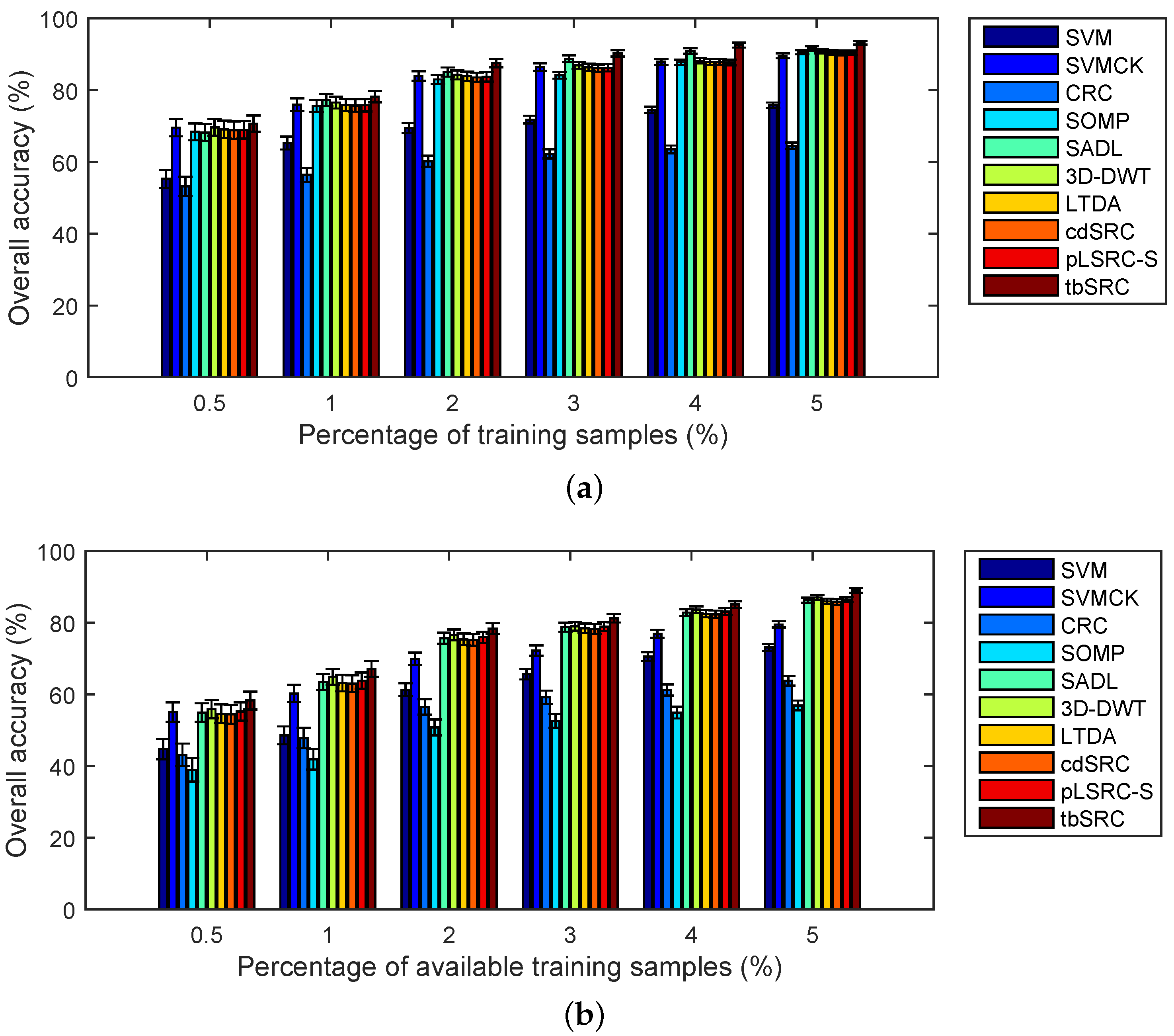
5.4. Classification Results and Discussions of Experiment 2

In experiment 2, we compare the aforementioned methods with various small numbers of labeled samples. The OA of different methods are depicted in Figure 12, from which we can discuss that:

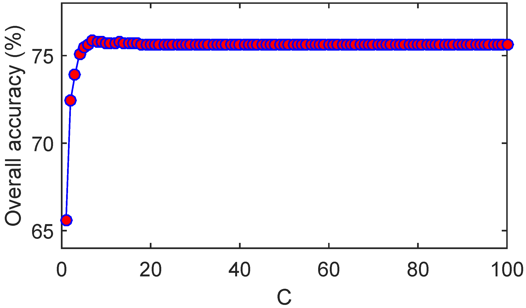
• As expected, the classification accuracy increases when the number of training samples increases. As depicted in Figure 12a, the OA of tbSRC is much lower than 90% when only 0.5% of labeled samples of the Indian Pines data are selected as training samples, while the OA is more than 90% with 5% of labeled samples as training samples;
• tbSRC is demonstrated to be superior to other methods with a small number of labeled samples, while SADL, 3D-DWT, LTDA, cdSRC and pLSRC-S trail marginally behind tbSRC. As observed from Figure 12a, although only 1% of labeled samples of the Indian Pines data are chosen selected as training samples, the OA of tbSRC almost reaches 80%, while the OAs of SADL, 3D-DWT, LTDA, cdSRC and pLSRC-S are slightly lower than that of tbSRC. Moreover, it is interesting to note that SADL, 3D-DWT, LTDA, cdSRC and pLSRC-S can achieve comparable performance. As shown in Figure 12a, the variations among OAs of those five methods are quite small. Similar results can also be discerned from Figure 12b;
• For the Indian Pines data, SOMP exhibits comparable classification accuracies to those of SVMCK. As illustrated in Figure 12a, the gap between SOMP and SVMCK is narrow, regardless what ratios of samples are chosen as training samples. However, SOMP delivers the worst results compared with the other seven methods for the other two data sets. Figure 12b reveals that the OA of SOMP is lower than 60% even when 5% of the available training samples is selected, whereas the OAs of the other methods (except CRC) are higher than 60% when using as low as 2% of the available training samples.

In a nutshell, the classification results of experiments 1 and 2 for two benchmark HSI data sets demonstrate the effectiveness of our proposed tbSRC in improving the classification performance.

6. Conclusions

In this paper, we have proposed a tensor block-sparsity based representation method (i.e., tbSRC) for spectral-spatial classification of HSI. The proposed tbSRC aims at taking the entire HSI cube as a third-order tensor and linearly representing a hyperspectral sample by a few atoms learned from the data. To that end, we perform tensor block-sparsity based dictionary learning and class-dependent block sparse representation on the HSI. Compared against techniques in the literature, our proposed tbSRC provides significant improvements and demonstrates promising results. On the one hand, tbSRC can effectively learn the optimal dictionary with the tensor block-sparsity constraint for a number of groups, which consist of several local patches centered at the training samples and are grouped by the class labels of training samples. The learned dictionary can effectively characterize the subspace structure of different classes and is much better than a dictionary directly constructed using training samples. On the other hand, block sparse representation is performed on the small local patch centered at the test sample in a class-wise manner to make full use of the class label information. Experiments conducted on two benchmark data sets have consistently confirmed the effectiveness of tbSRC, even in scenarios with a small number of training samples. Quantitatively, the OA of tbSRC improves about 2% to 30% compared to other state-of-the-art methods. In the future, a further improvement will be achieved by investigating the kernel variant of tbSRC.

References

1. Bioucas-Dias, J.M.; Plaza, A.; Camps-Valls, G.; Scheunders, P.; Nasrabadi, N.M.; Chanussot, J. Hyperspectral remote sensing data analysis and future challenges. IEEE Geosci. Remote Sens. Mag. 2013, 1, 6–36. [Google Scholar] [CrossRef]
2. Song, H.; Wang, Y. A spectral-spatial classification of hyperspectral images based on the algebraic multigrid method and hierarchical segmentation algorithm. Remote Sens. 2016, 8. [Google Scholar] [CrossRef]
3. Sun, X.; Yang, L.; Zhang, B.; Gao, L.; Gao, J. An endmember extraction method based on artificial bee colony algorithms for hyperspectral remote sensing images. Remote Sens. 2015, 7, 16363–16383. [Google Scholar] [CrossRef]
4. Sun, W.; Jiang, M.; Li, W.; Liu, Y. A symmetric sparse representation based band selection method for hyperspectral imagery classification. Remote Sens. 2016, 8. [Google Scholar] [CrossRef]
5. Sun, W.; Zhang, L.; Zhang, L.; Lai, Y.M. A dissimilarity-weighted sparse self-representation method for band selection in hyperspectral imagery classification. IEEE J. Sel. Top. Appl. Earth Obs. Remote Sens. 2016. [Google Scholar] [CrossRef]
6. Jia, X.; Kuo, B.C.; Crawford, M.M. Feature mining for hyperspectral image classification. Proc. IEEE 2013, 101, 676–697. [Google Scholar] [CrossRef]
7. Chen, Y.; Zhao, X.; Jia, X. Spectral-spatial classification of hyperspectral data based on deep belief network. IEEE J. Sel. Top. Appl. Earth Obs. Remote Sens. 2015, 8, 2381–2392. [Google Scholar] [CrossRef]
8. Wu, Z.; Wang, Q.; Plaza, A.; Li, J.; Liu, J.; Wei, Z. Parallel implementation of sparse representation classifiers for hyperspectral imagery on GPUs. IEEE J. Sel. Top. Appl. Earth Obs. Remote Sens. 2015, 8, 2912–2925. [Google Scholar] [CrossRef]
9. Liang, H.; Li, Q. Hyperspectral imagery classification using sparse representations of convolutional neural network features. Remote Sens. 2016, 8, 99. [Google Scholar] [CrossRef]
10. Vapnik, V.N. The Nature of Statistical Learning Theory; Springer-Verlag: New York, NY, USA, 1995. [Google Scholar]
11. Ramzi, P.; Samadzadegan, F.; Reinartz, P. Classification of hyperspectral data using an AdaBoostSVM technique applied on band clusters. IEEE J. Sel. Top. Appl. Earth Obs. Remote Sens. 2014, 7, 2066–2079. [Google Scholar] [CrossRef]
12. Baldeck, C.; Asner, G.P. Single-species detection with airborne imaging spectroscopy data: A comparison of support vector techniques. IEEE J. Sel. Top. Appl. Earth Obs. Remote Sens. 2015, 8, 2501–2512. [Google Scholar] [CrossRef]
13. Chen, Y.; Nasrabadi, N.M.; Tran, T.D. Hyperspectral image classification via kernel sparse representation. IEEE Trans. Geosci. Remote Sens. 2013, 51, 217–231. [Google Scholar] [CrossRef]
14. Fang, L.; Li, S.; Kang, X.; Benediktsson, J.A. Spectral-spatial hyperspectral image classification via multiscale adaptive sparse representation. IEEE Trans. Geosci. Remote Sens. 2014, 52, 7738–7749. [Google Scholar] [CrossRef]
15. Sun, X.; Nasrabadi, N.M.; Tran, T.D. Task-driven dictionary learning for hyperspectral image classification with structured sparsity constraints. IEEE Trans. Geosci. Remote Sens. 2015, 53, 4457–4471. [Google Scholar] [CrossRef]
16. Ly, N.H.; Du, Q.; Fowler, J.E. Collaborative graph-based discriminant analysis for hyperspectral imagery. IEEE J. Sel. Top. Appl. Earth Obs. Remote Sens. 2014, 7, 2688–2696. [Google Scholar] [CrossRef]
17. Ly, N.H.; Du, Q.; Fowler, J.E. Sparse graph-based discriminant analysis for hyperspectral imagery. IEEE Trans. Geosci. Remote Sens. 2014, 52, 3872–3884. [Google Scholar]
18. Li, J.; Huang, X.; Gamba, P.; Bioucas, J.; Zhang, L.; Benediksson, J.; Plaza, A. Multiple feature learning for hyperspectral image classification. IEEE Trans. Geosci. Remote Sens. 2015, 53, 1592–1606. [Google Scholar] [CrossRef]
19. Camps-Valls, G.; Gomez-Chova, L.; Muñoz-Marí, J.; Vila-Francés, J.; Calpe-Maravilla, J. Composite kernels for hyperspectral image classification. IEEE Geosci. Remote Sens. Lett. 2006, 3, 93–97. [Google Scholar] [CrossRef]
20. Tuia, D.; Camps-Valls, G.; Matasci, G.; Kanevski, M. Learning relevant image features with multiple-kernel classification. IEEE Trans. Geosci. Remote Sens. 2010, 48, 3780–3791. [Google Scholar] [CrossRef]
21. He, Z.; Wang, Q.; Shen, Y.; Sun, M. Kernel sparse multitask learning for hyperspectral image classification with empirical mode decomposition and morphological wavelet-based features. IEEE Trans. Geosci. Remote Sens. 2014, 52, 5150–5163. [Google Scholar]
22. Li, J.; Marpu, P.R.; Plaza, A.; Bioucas-Dias, J.M.; Benediktsson, J.A. Generalized composite kernel framework for hyperspectral image classification. IEEE Trans. Geosci. Remote Sens. 2013, 51, 4816–4829. [Google Scholar] [CrossRef]
23. He, Z.; Li, J. Multiple data-dependent kernel for classification of hyperspectral images. Expert Syst. Appl. 2015, 42, 1118–1135. [Google Scholar] [CrossRef]
24. Tarabalka, Y.; Fauvel, M.; Chanussot, J.; Benediktsson, J.A. SVM-and MRF-based method for accurate classification of hyperspectral images. IEEE Geosci. Remote Sens. Lett. 2010, 7, 736–740. [Google Scholar] [CrossRef]
25. Li, J.; Bioucas-Dias, J.; Plaza, A. Spectral-spatial hyperspectral image segmentation using subspace multinomial logistic regression and Markov random fields. IEEE Trans. Geosci. Remote Sens. 2012, 50, 809–823. [Google Scholar] [CrossRef]
26. Srinivas, U.; Chen, Y.; Monga, V.; Nasrabadi, N.M.; Tran, T.D. Exploiting sparsity in hyperspectral image classification via graphical models. IEEE Geosci. Remote Sens. Lett. 2013, 10, 505–509. [Google Scholar] [CrossRef]
27. Zhang, H.; Li, J.; Huang, Y.; Zhang, L. A nonlocal weighted joint sparse representation classification method for hyperspectral imagery. IEEE J. Sel. Top. Appl. Earth Obs. Remote Sens. 2014, 7, 2056–2065. [Google Scholar] [CrossRef]
28. Chen, Y.; Nasrabadi, N.M.; Tran, T.D. Hyperspectral image classification using dictionary-based sparse representation. IEEE Trans. Geosci. Remote Sens. 2010, 49, 3973–3985. [Google Scholar] [CrossRef]
29. Soltani-Farani, A.; Rabiee, H.R.; Hosseini, S.A. Spatial-aware dictionary learning for hyperspectral image classification. IEEE Trans. Geosci. Remote Sens. 2015, 53, 527–541. [Google Scholar] [CrossRef]
30. Sun, X.; Qu, Q.; Nasrabadi, N.M.; Tran, T.D. Structured priors for sparse-representation-based hyperspectral image classification. IEEE Geosci. Remote Sens. Lett. 2014, 11, 1235–1239. [Google Scholar]
31. Du, P.; Xue, Z.; Li, J.; Plaza, A. Learning discriminative sparse representations for hyperspectral image classification. IEEE J. Sel. Top. Appl. Earth Obs. Remote Sens. 2015, 9, 1089–1104. [Google Scholar] [CrossRef]
32. Wang, Z.; Nasrabadi, N.M.; Huang, T.S. Spatial-spectral classification of hyperspectral images using discriminative dictionary designed by learning vector quantization. IEEE Trans. Geosci. Remote Sens. 2014, 52, 4808–4822. [Google Scholar] [CrossRef]
33. Zhang, L.; Yang, M.; Feng, X. Sparse representation or collaborative representation: Which helps face recognition? In Proceedings of the 2011 International Conference on Computer Vision, Barcelona, Spain, 6–13 November 2011; pp. 471–478.
34. Rubinstein, R.; Bruckstein, A.M.; Elad, M. Dictionaries for sparse representation modeling. Proc. IEEE. 2010, 98, 1045–1057. [Google Scholar] [CrossRef]
35. Cui, M.; Prasad, S. Class-dependent sparse representation classifier for robust hyperspectral image classification. IEEE Trans. Geosci. Remote Sens. 2015, 53, 2683–2695. [Google Scholar] [CrossRef]
36. Qian, Y.; Ye, M.; Zhou, J. Hyperspectral image classification based on structured sparse logistic regression and three-dimensional wavelet texture features. IEEE Trans. Geosci. Remote Sens. 2012, 51, 2276–2291. [Google Scholar] [CrossRef]
37. Lin, T.; Bourennane, S. Hyperspectral image processing by jointly filtering wavelet component tensor. IEEE Trans. Geosci. Remote Sens. 2013, 51, 3529–3541. [Google Scholar] [CrossRef]
38. Jia, S.; Zhu, Z.; Shen, L.; Li, Q. A two-stage feature selection framework for hyperspectral image classification using few labeled samples. IEEE J. Sel. Top. Appl. Earth Obs. Remote Sens. 2014, 7, 1023–1035. [Google Scholar] [CrossRef]
39. Zhang, L.; Zhang, L.; Tao, D.; Huang, X. Tensor discriminative locality alignment for hyperspectral image spectral–spatial feature extraction. IEEE Trans. Geosci. Remote Sens. 2013, 51, 242–256. [Google Scholar] [CrossRef]
40. Tsai, F.; Lai, J.S. Feature extraction of hyperspectral image cubes using three-dimensional gray-level cooccurrence. IEEE Trans. Geosci. Remote Sens. 2013, 51, 3504–3513. [Google Scholar] [CrossRef]
41. Yang, S.; Wang, M.; Li, P.; Jin, L.; Wu, B.; Jiao, L. Compressive hyperspectral imaging via sparse tensor and nonlinear compressed sensing. IEEE Trans. Geosci. Remote Sens. 2015, 53, 5943–5957. [Google Scholar] [CrossRef]
42. Zhong, Z.; Fan, B.; Duan, J.; Wang, L.; Ding, K.; Xiang, S.; Pan, C. Discriminant tensor spectral-spatial feature extraction for hyperspectral image classification. IEEE Geosci. Remote Sens. Lett. 2015, 12, 1028–1032. [Google Scholar] [CrossRef]
43. Peng, Y.; Meng, D.; Xu, Z.; Gao, C.; Yang, Y.; Zhang, B. Decomposable nonlocal tensor dictionary learning for multispectral image denoising. In Proceedings of the 2014 IEEE Conference on Computer Vision and Pattern Recognition (CVPR), Columbus, OH, USA, 23–28 June 2014; pp. 2949–2956.
44. Sivalingam, R.; Boley, D.; Morellas, V.; Papanikolopoulos, N. Tensor dictionary learning for positive definite matrices. IEEE Trans. Image Process. 2015, 24, 4592–4601. [Google Scholar] [CrossRef] [PubMed]
45. Tan, S.; Zhang, Y.; Wang, G.; Mou, X.; Cao, G.; Wu, Z.; Yu, H. Tensor-based dictionary learning for dynamic tomographic reconstruction. Phys. Med. Biol. 2015, 60, 2803–2818. [Google Scholar] [CrossRef] [PubMed]
46. Duarte, M.F.; Baraniuk, R.G. Kronecker compressive sensing. IEEE Trans. Image Process. 2012, 21, 494–504. [Google Scholar] [CrossRef] [PubMed]
47. Caiafa, C.F.; Cichocki, A. Computing sparse representations of multidimensional signals using kronecker bases. Neural Comput. 2013, 25, 186–220. [Google Scholar] [CrossRef] [PubMed]
48. Caiafa, C.F.; Cichocki, A. Multidimensional compressed sensing and their applications. Wiley Interdiscip. Rev. Data Min. Knowl. Discov. 2013, 3, 355–380. [Google Scholar] [CrossRef]
49. Kolda, T.G.; Bader, B.W. Tensor decompositions and applications. SIAM Rev. 2009, 51, 455–500. [Google Scholar] [CrossRef]
50. Guo, X.; Huang, X.; Zhang, L.; Zhang, L. Hyperspectral image noise reduction based on rank-1 tensor decomposition. ISPRS J. Photogramm. Remote Sens. 2013, 83, 50–63. [Google Scholar] [CrossRef]
51. Velasco-Forero, S.; Angulo, J. Classification of hyperspectral images by tensor modeling and additive morphological decomposition. Pattern Recognit. 2013, 46, 566–577. [Google Scholar] [CrossRef] [Green Version]
52. Tropp, J.A.; Gilbert, A.C. Signal recovery from random measurements via orthogonal matching pursuit. IEEE Trans. Inf. Theory 2007, 53, 4655–4666. [Google Scholar] [CrossRef]
53. Chen, S.S.; Donoho, D.L.; Saunders, M.A. Atomic decomposition by basis pursuit. SIAM J. Sci. Comput. 1998, 20, 33–61. [Google Scholar] [CrossRef]
54. Schwarz, G. Estimating the dimension of a model. Ann. Stat. 1978, 6, 461–464. [Google Scholar] [CrossRef]
55. Tucker, L.R. Some mathematical notes on three-mode factor analysis. Psychometrika 1966, 31, 279–311. [Google Scholar] [CrossRef] [PubMed]
56. Fauvel, M.; Tarabalka, Y.; Benediktsson, J.A.; Chanussot, J.; Tilton, J.C. Advances in spectral-spatial classification of hyperspectral images. Proc. IEEE 2013, 101, 652–675. [Google Scholar] [CrossRef]
Figure 1. Vector and tensor representations of a 5 × 5 local patch from the original HSI data set.
Remotesensing 08 00636 g001
Figure 2. Flowchart of the proposed algorithm. In each class, Z ̲ ( k ) share the same atoms of dictionaries ( D k w , D k h , D k s ) , thus making the dictionary learning process tensor block-sparse.
Remotesensing 08 00636 g002
Figure 3. Illustration of different types of sparsity: (a) Unstructured sparse core tensor; (b) Block- structured sparse core tensor.
Remotesensing 08 00636 g003
Figure 4. A synthetic example conducted on a subset of the Salinas-A scene.
Remotesensing 08 00636 g004
Figure 5. Indian Pines image: (a) Three-band false color composite; (b) Ground truth data with 16 classes.
Remotesensing 08 00636 g005
Figure 6. University of Pavia image: (a) Three-band false color composite; (b) Ground truth data with 9 classes; (c) Available training samples.
Remotesensing 08 00636 g006
Figure 7. The effect of C ( C { 1 , 2 , , 100 } with γ = 1 ) on OA of SVM for the Indian Pines data.
Remotesensing 08 00636 g007
Figure 8. The effect of neighborhood size on OA of tbSRC for the two HSI data sets.
Remotesensing 08 00636 g008
Figure 9. Illustration of the block-structured sparsity derived from the real-world Indian Pines data set. Without loss of generality, the test sample (belonging to class 1 alfalfa) is chosen from the spatial coordinate ( 70 , 97 ) and let the neighborhood size be 9 × 9 and k = 1 , the normalized small local patch of the test sample X ̲ ˜ R 9 × 9 × 200 can be approximately represented by the 1st group dictionaries ( D 1 w , D 1 h , D 1 s ) and the core tensor Z ̲ ˜ ( 1 ) with D 1 w , D 1 h R 9 × 9 , D 1 s R 200 × 129 , and Z ̲ ˜ ( 1 ) R 9 × 9 × 129 . It is notable that the non-zero elements of Z ̲ ˜ ( 1 ) have block structure, which is consistent with the ideal situation shown in Figure 3b.
Remotesensing 08 00636 g009
Figure 10. Classification maps of the Indian Pines data obtained by (a) SVM; (b) SVMCK; (c) CRC; (d) SOMP; (e) SADL; (f) 3D-DWT; (g) LTDA; (h) cdSRC; (i) pLSRC; and (j) tbSRC.
Remotesensing 08 00636 g010
Figure 11. Classification maps of the University of Pavia data obtained by (a) SVM; (b) SVMCK; (c) CRC; (d) SOMP; (e) SADL; (f) 3D-DWT; (g) LTDA; (h) cdSRC; (i) pLSRC; and (j) tbSRC.
Remotesensing 08 00636 g011
Figure 12. Overall accuracy (%) of different methods with various numbers of labeled samples for (a) Indian Pines data and (b) University of Pavia data.
Remotesensing 08 00636 g012