
Superpixel-Based Classification Using K Distribution and Spatial Context for Polarimetric SAR Images


Abstract
:
1. Introduction
1.1. Background
1.2. Related Works
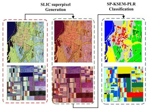
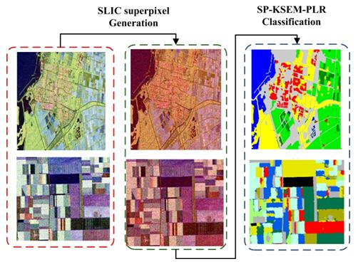
1.3. The Proposed Approach
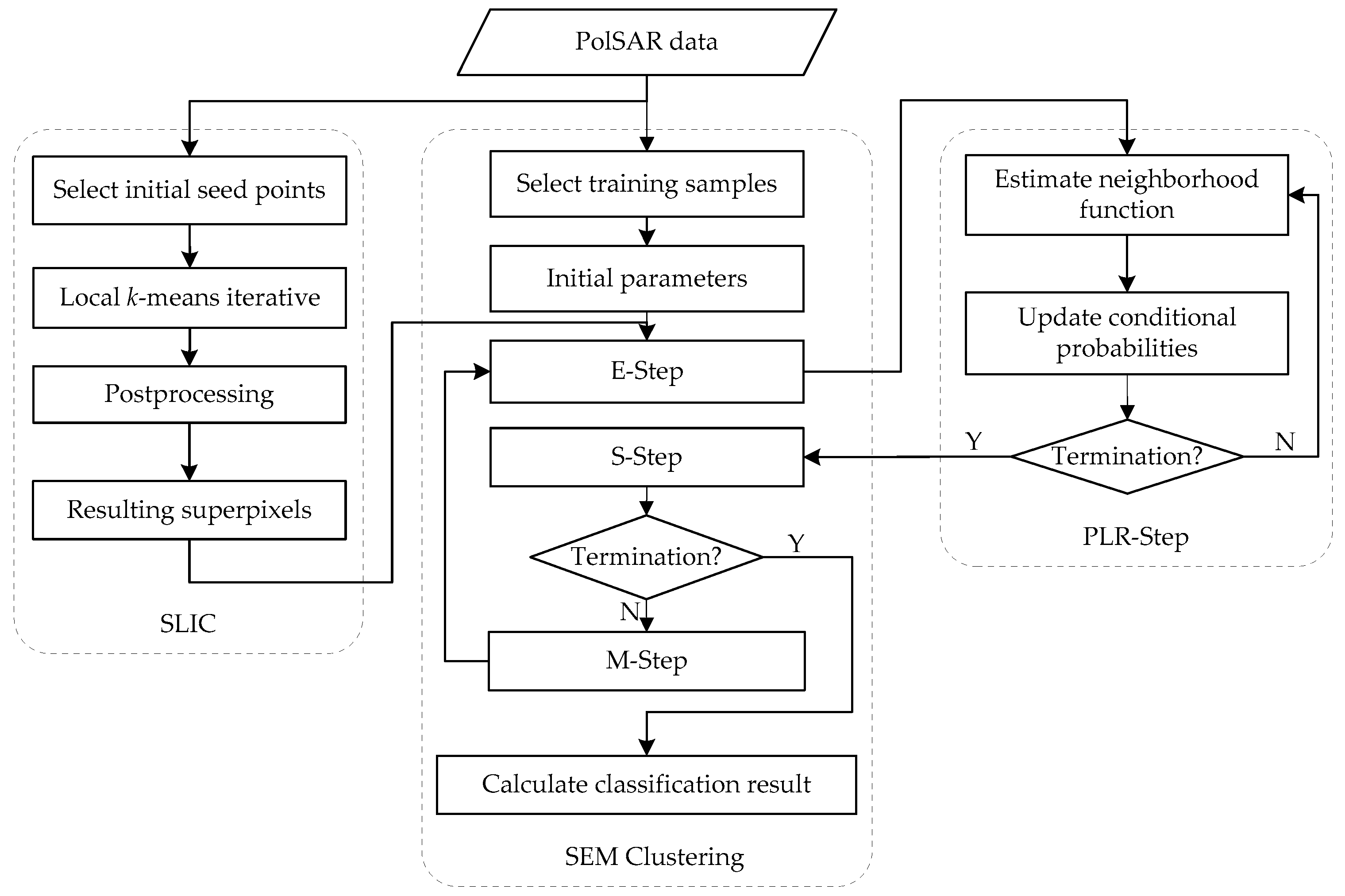
2. Methodology
2.1. Superpixel Generation in PolSAR Images
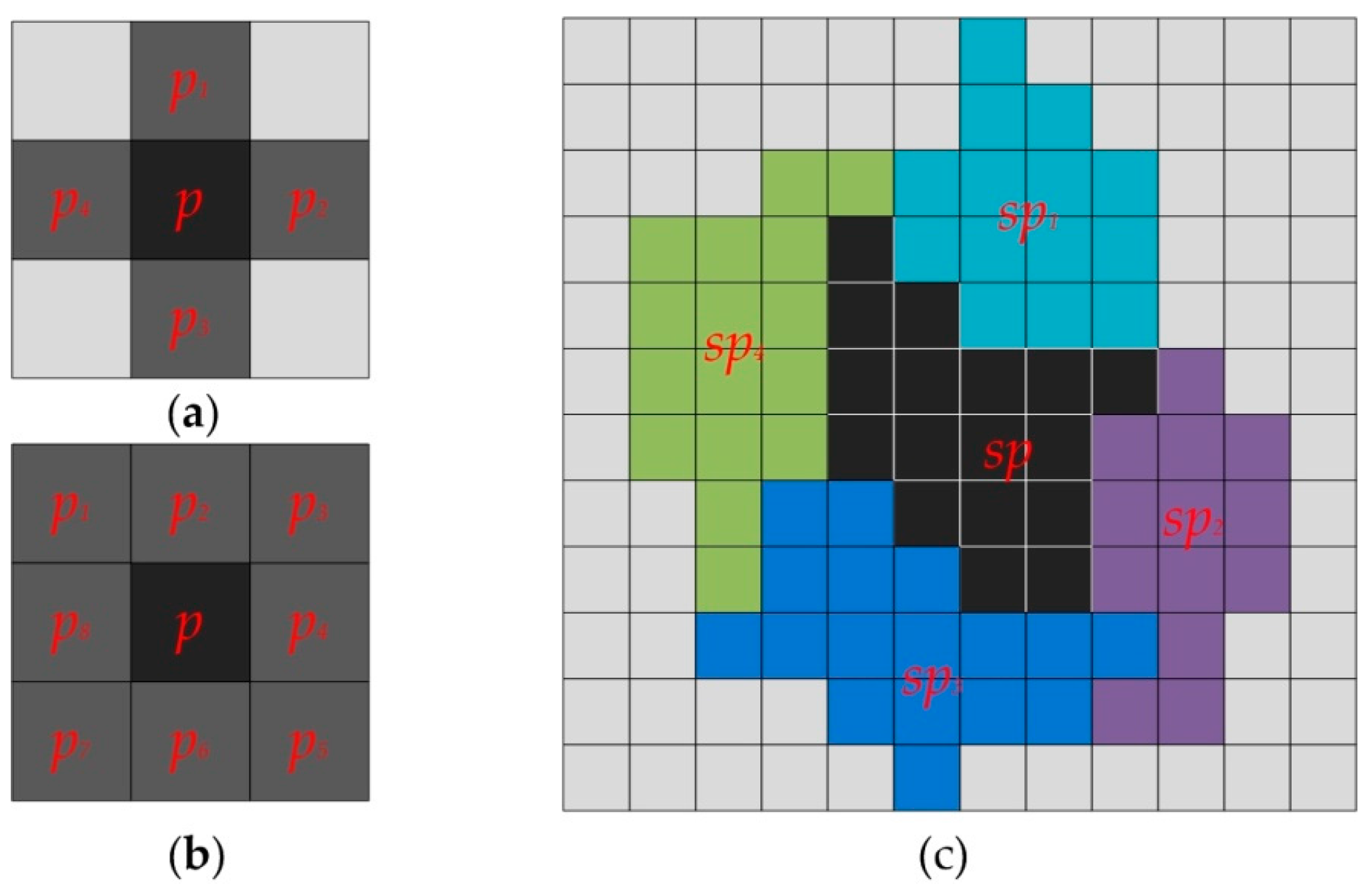
2.2. Superpixel-Based PLR Model
2.3. SEM Clustering Utilizing the K Distribution
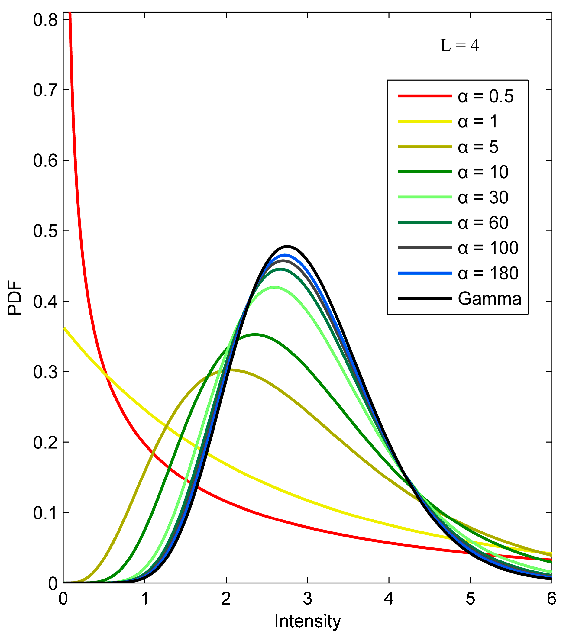
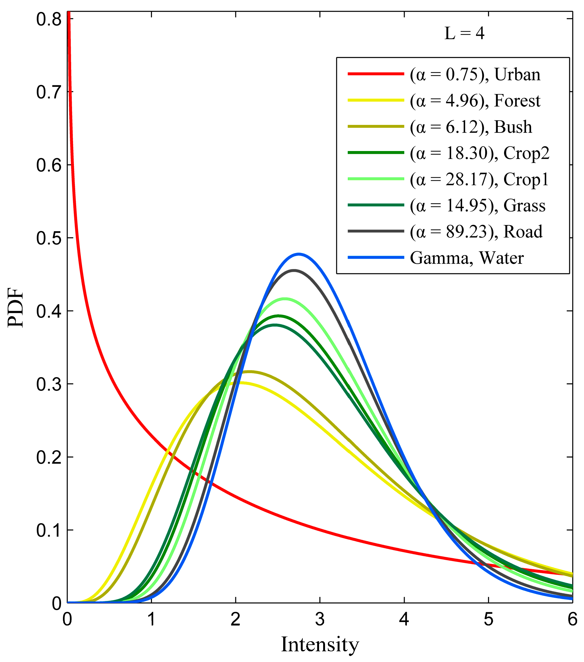
2.3.1. PolSAR K Distribution
2.3.2. SEM Clustering Processing
| Algorithm 1: Superpixel-based SEM clustering utilizing the K distribution. |
| 1: INPUT: PolSAR image, training samples, maximum iterations of SEM MAX. |
| 2: OUTPUT: classification image . |
| 3: Generate superpixels of PolSAR image by SLIC method by Equations (1) and (2). |
| 4: Compute initial K distribution parameters by the MoMLC method by Equation (15) with training samples. |
| 5: Do |
| 6: |
| 7: for each superpixel do |
| 8: Compute posterior probabilities of each class by Equations (13) and (18). |
| 9: end for |
| 10: for each superpixel do |
| 11: Update following Equations (4)–(6) |
| 12: end for |
| 13: for each superpixel do |
| 14: Compute by randomly labeling according to . |
| 15: end for |
| 16: if () do compute termination criterion following Equation (19). |
| 17: if () goto Step 19, and compute final classification results. |
| 18: While ( MAX) |
| 19: for each superpixel do |
| 20: Compute classification result by the MAP decision rule according to . |
| 21: end for |
3. Experiment and Results
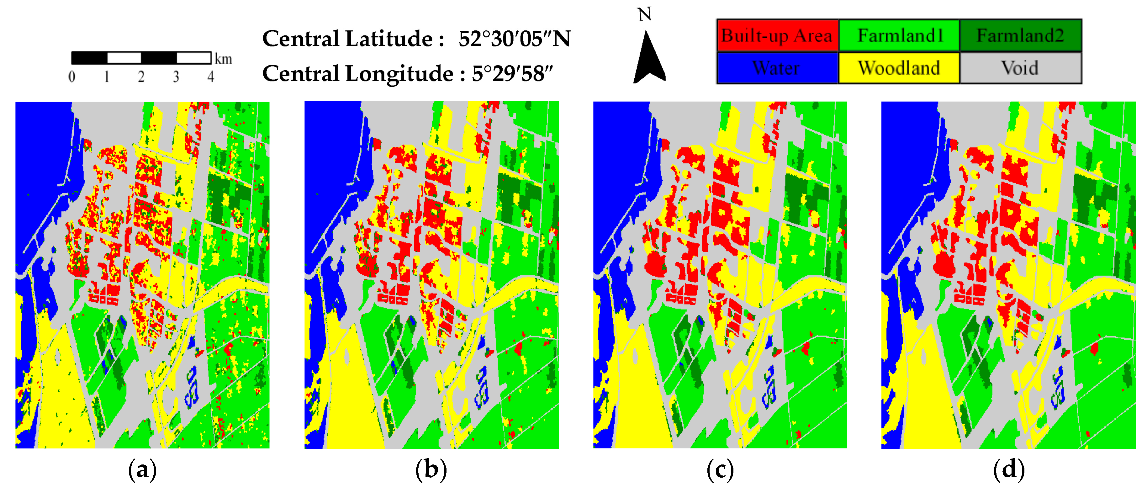
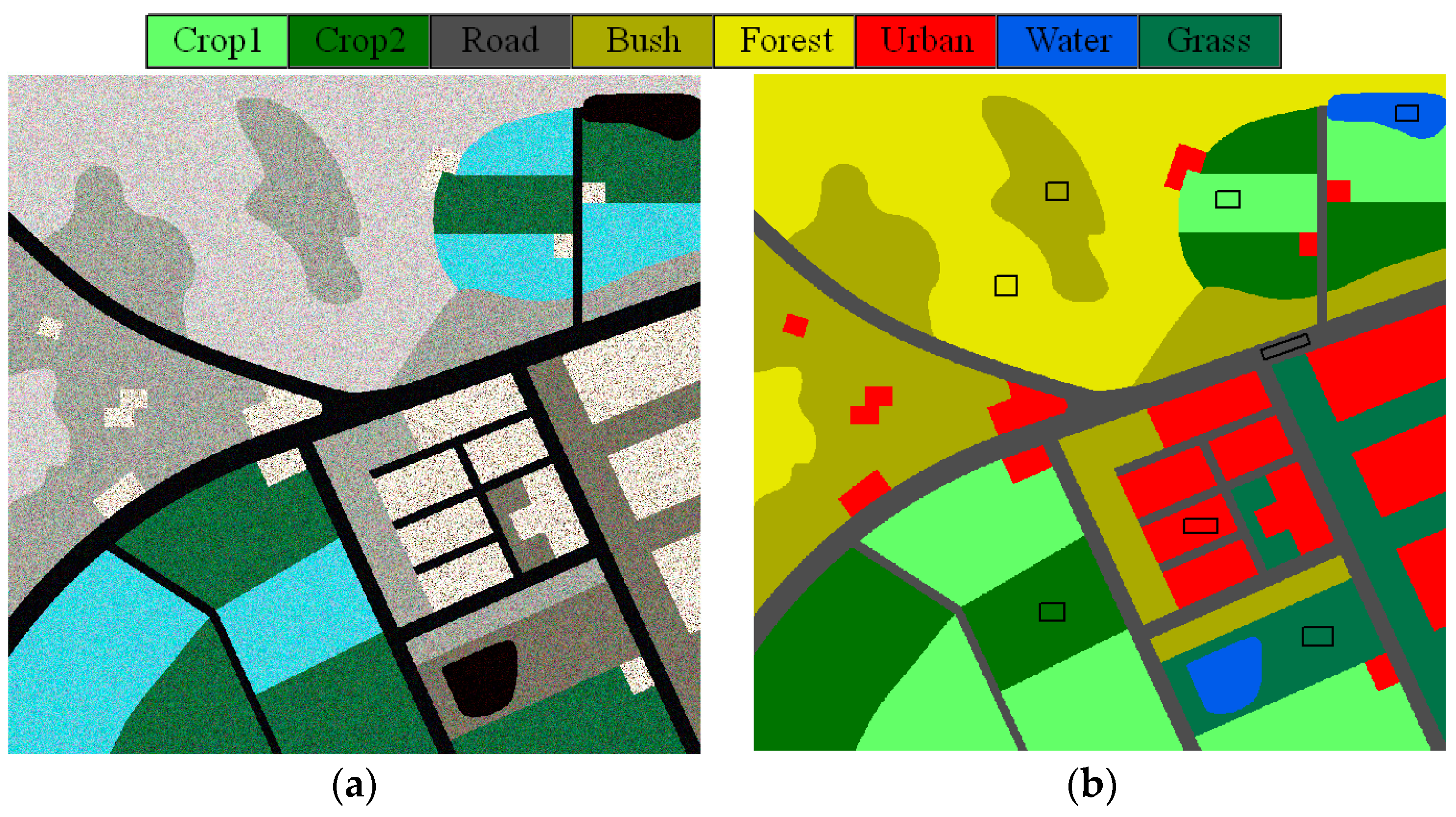
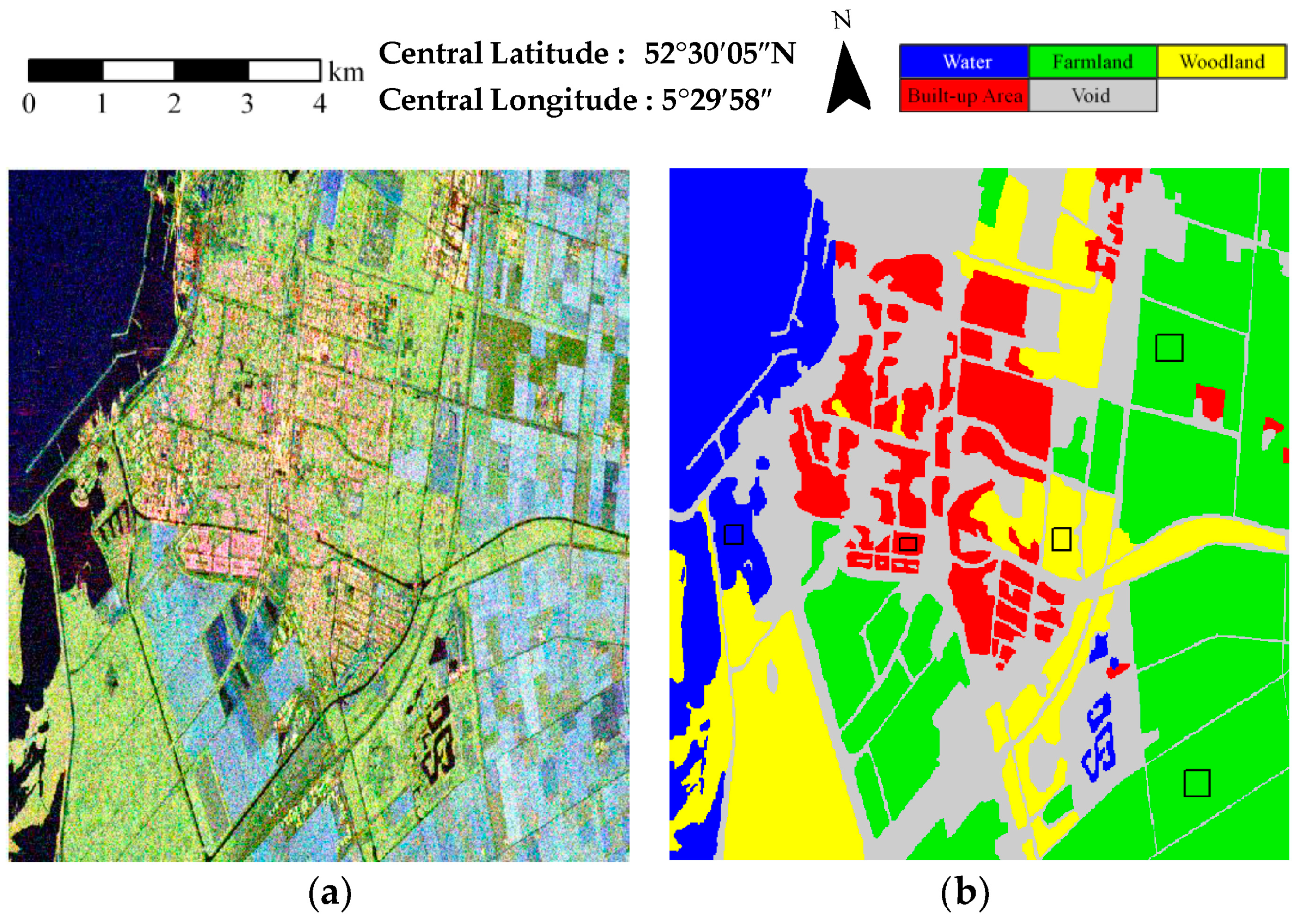
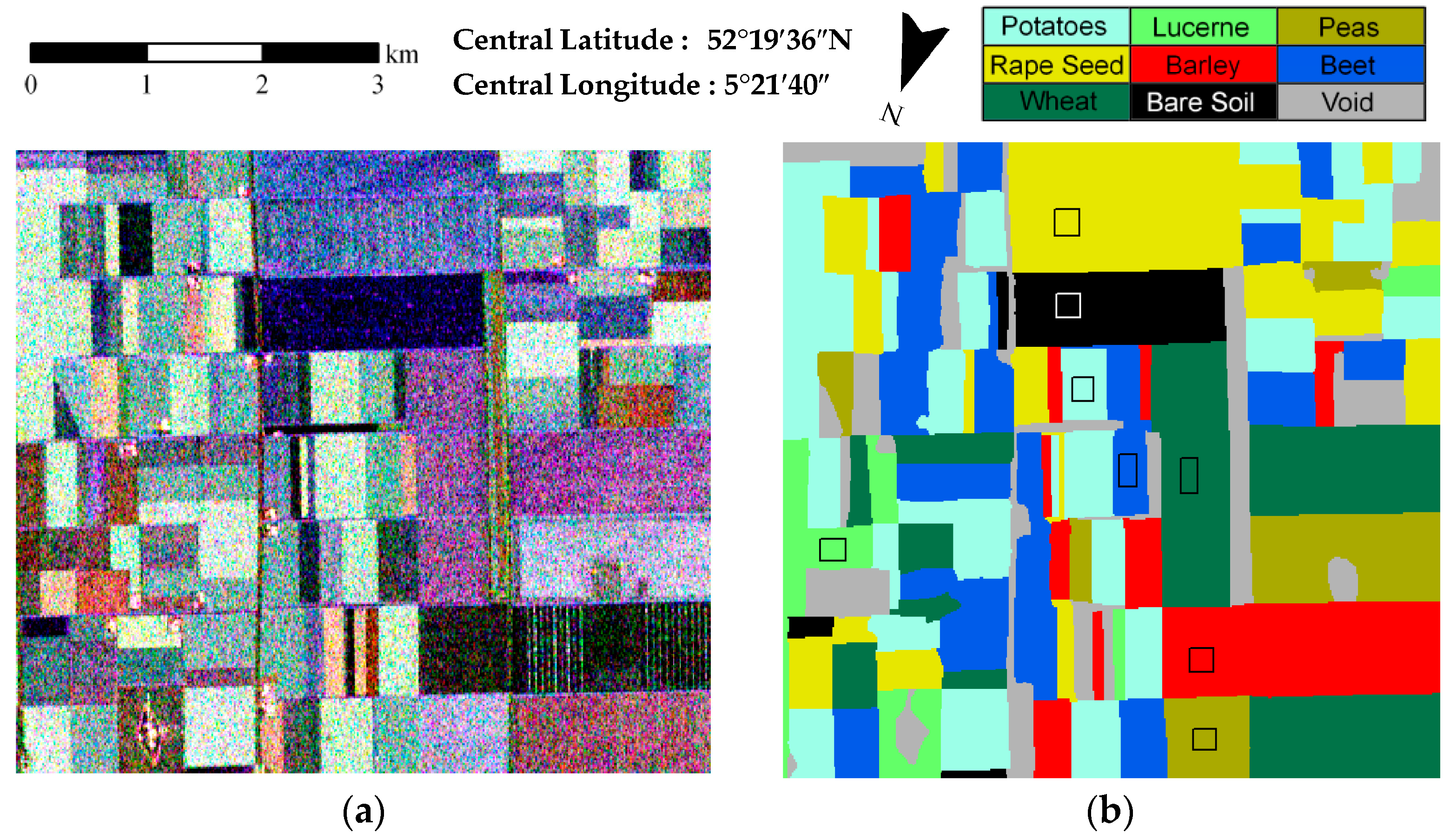
3.1. Description of the Experimental Datasets
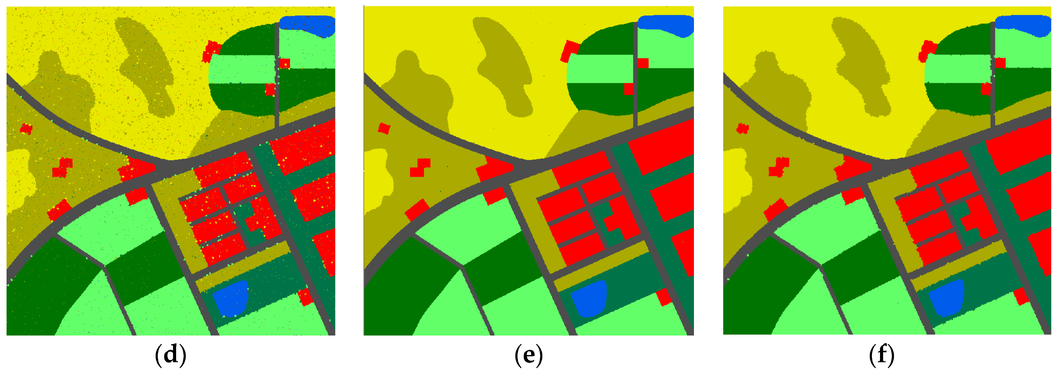
3.2. Evaluation and Comparison
4. Discussion
4.1. Main Features of the Proposed Method
4.2. Sensitivity Analysis of the Parameters
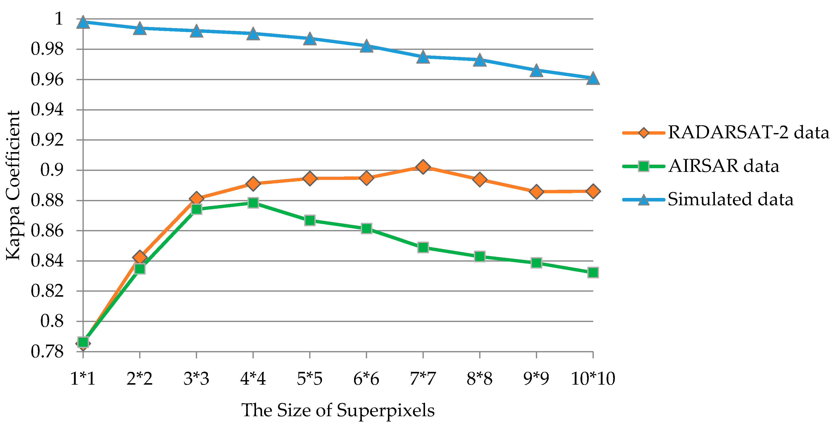
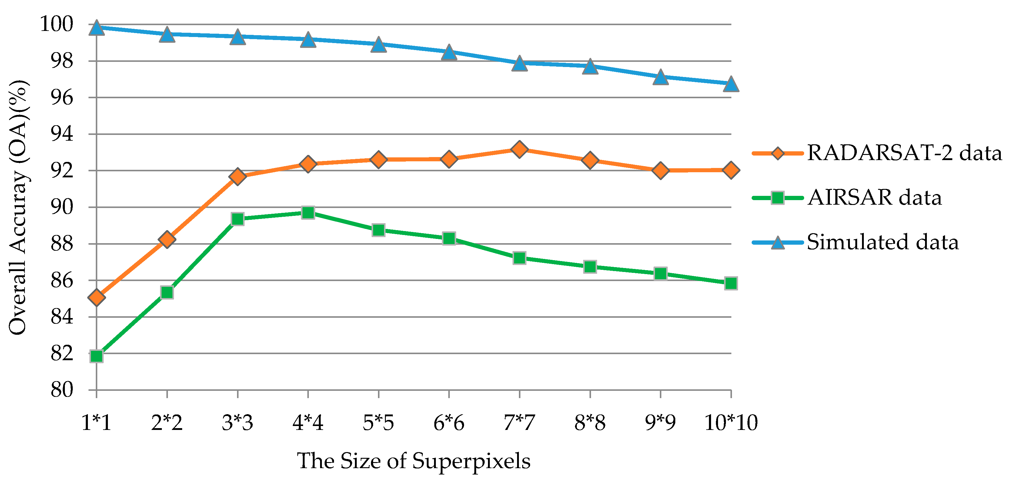
4.2.1. Size of Superpixels
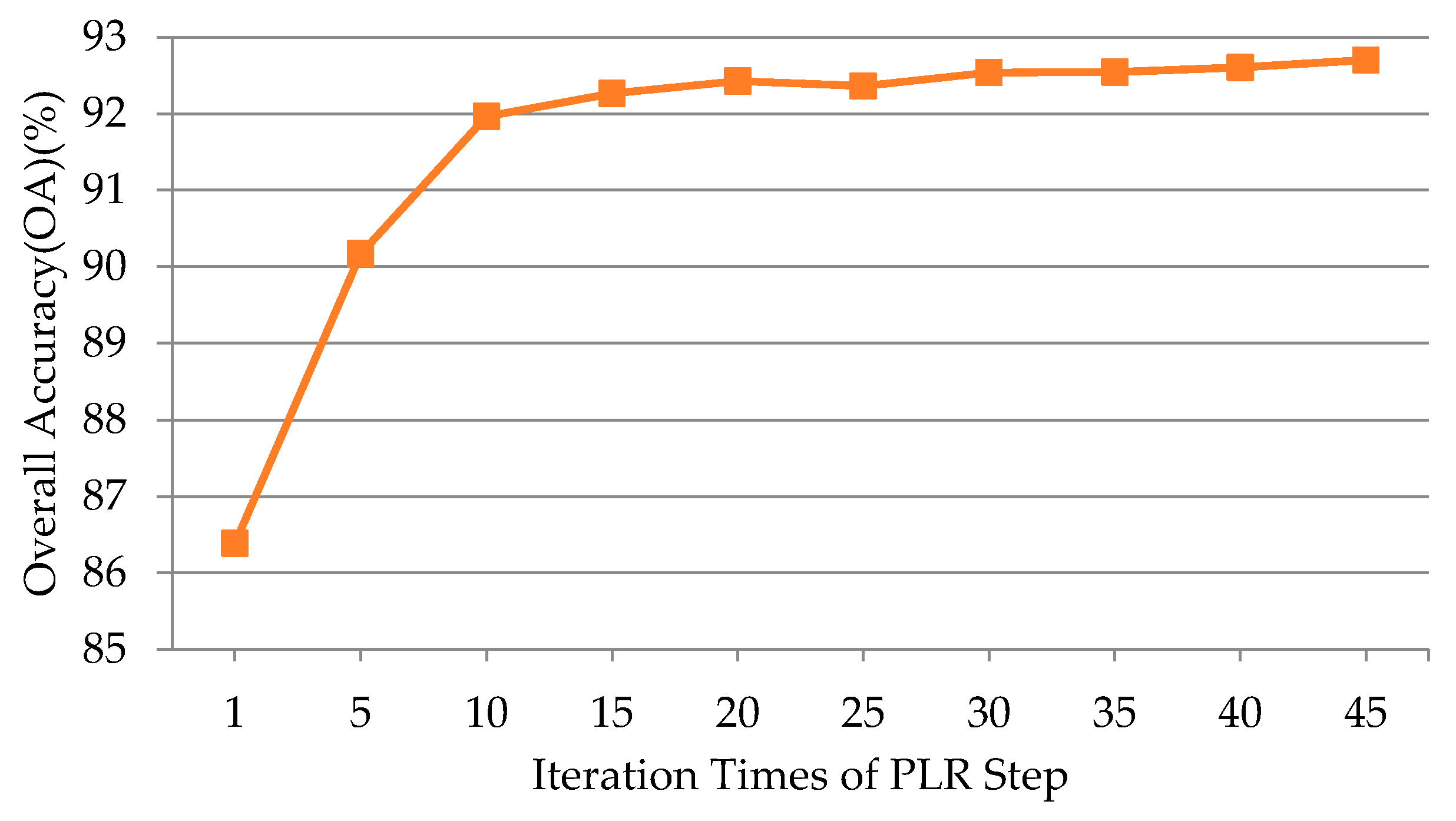
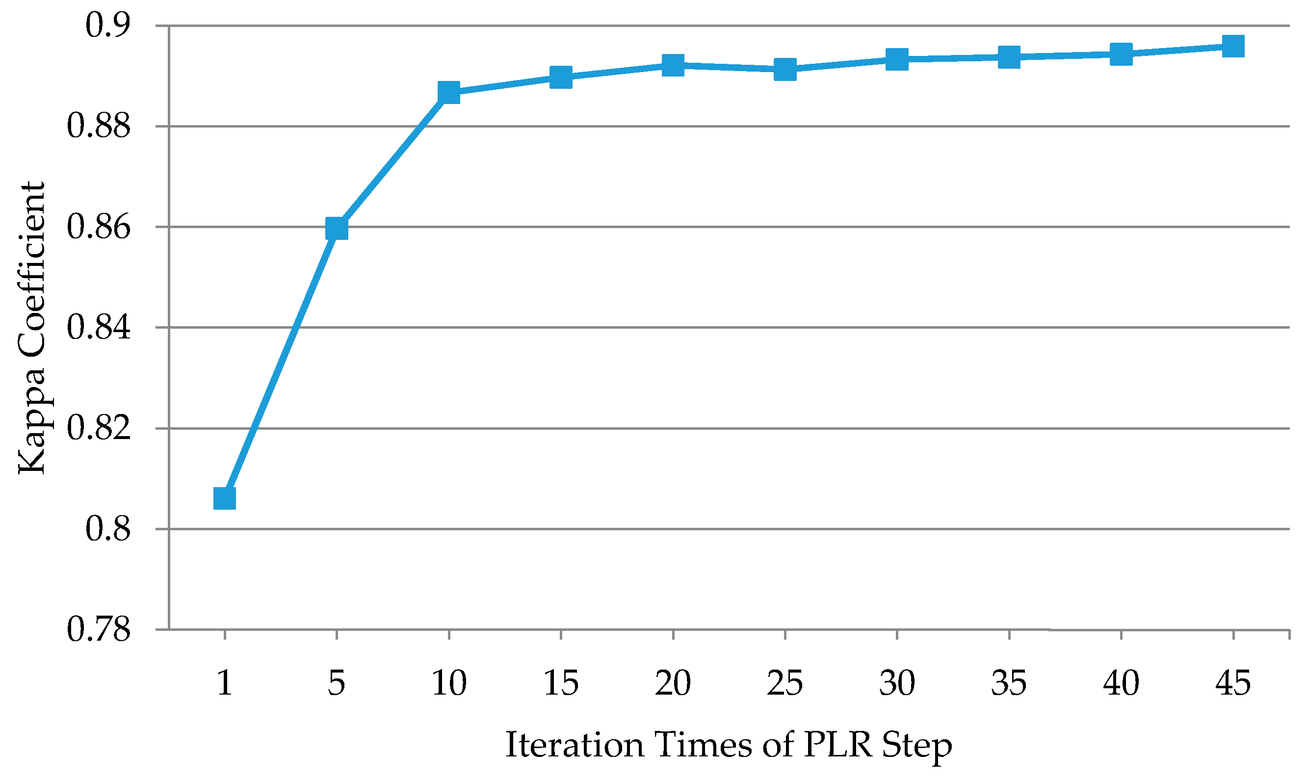
4.2.2. Iteration Times of the PLR Step
4.3. Accuracies, Errors and Uncertainties
5. Conclusions
Acknowledgments
Author Contributions
Conflicts of Interest
References
- Wei, J.; Zhang, J.; Huang, G.; Zhao, Z. On the use of Cross-Correlation between volume scattering and helix scattering from polarimetric SAR data for the improvement of ship detection. Remote Sens. 2016, 8, 74. [Google Scholar] [CrossRef]
- Ressel, R.; Singha, S. Comparing near coincident space borne C and X band fully polarimetric SAR data for arctic sea ice classification. Remote Sens. 2016, 8, 198. [Google Scholar] [CrossRef]
- Cloude, S.R.; Pottier, E. An entropy based classification scheme for land applications of polarimetric SAR. IEEE Trans. Geosci. Remote Sens. 1997, 35, 68–78. [Google Scholar] [CrossRef]
- Touzi, R.; Boerner, W.M.; Lee, J.S.; Lueneburg, E. A review of polarimetry in the context of synthetic aperture radar: Concepts and information extraction. Can. J. Remote Sens. 2004, 30, 380–407. [Google Scholar] [CrossRef]
- Huang, X.; Wang, J.; Shang, J. An integrated surface parameter inversion scheme over agricultural fields at early growing stages by means of C-band polarimetric RADARSAT-2 imagery. IEEE Trans. Geosci. Remote Sens. 2016, 54, 2510–2528. [Google Scholar] [CrossRef]
- Akbari, V.; Doulgeris, A.P.; Moser, G.; Eltoft, T.; Anfinsen, S.N.; Serpico, S.B. A textural–contextual model for unsupervised segmentation of multipolarization synthetic aperture radar images. IEEE Trans. Geosci. Remote Sens. 2013, 51, 2442–2453. [Google Scholar] [CrossRef] [Green Version]
- Conradsen, K.; Nielsen, A.A.; Schou, J.; Skriver, H. A test statistic in the complex Wishart distribution and its application to change detection in polarimetric SAR data. IEEE Trans. Geosci. Remote Sens. 2003, 41, 4–19. [Google Scholar] [CrossRef]
- Lee, J.-S.; Ainsworth, T.L.; Wang, Y.; Chen, K.S. Polarimetric SAR speckle filtering and the extended sigma filter. IEEE Trans. Geosci. Remote Sens. 2015, 53, 1150–1160. [Google Scholar] [CrossRef]
- Du, L.J.; Lee, J.-S. Classification of multi-look polarimetric SAR imagery based on complex Wishart distribution. Int. J. Remote Sens. 1994, 15, 2299–2311. [Google Scholar]
- Lee, J.-S.; Grunes, M.R.; Ainsworth, T.L.; Du, L.; Schuler, D.L.; Cloude, S.R. Unsupervised classification using polarimetric decomposition and the complex Wishart classifier. IEEE Trans. Geosci. Remote Sens. 1999, 37, 2249–2258. [Google Scholar]
- Alonso-Gonzalez, A.; Lopez-Martinez, C.; Salembier, P. Filtering and segmentation of polarimetric SAR data based on binary partition Trees. IEEE Trans. Geosci. Remote Sens. 2012, 50, 593–605. [Google Scholar] [CrossRef]
- Kersten, P.R.; Lee, J.-S.; Ainsworth, T.L. Unsupervised classification of polarimetric synthetic aperture Radar images using fuzzy clustering and EM clustering. IEEE Trans. Geosci. Remote Sens. 2005, 43, 519–527. [Google Scholar] [CrossRef]
- Van Zyl, J.J. Unsupervised classification of scattering behavior using radar polarimetry data. IEEE Trans. Geosci. Remote Sens. 1989, 27, 36–45. [Google Scholar] [CrossRef]
- Ferro-Famil, L.; Pottier, E.; Lee, J. Unsupervised classification of multifrequency and fully polarimetric SAR images based on the H/A/Alpha-Wishart classifier. IEEE Trans. Geosci. Remote Sens. 2001, 39, 2332–2342. [Google Scholar] [CrossRef]
- Morandeira, N.; Grings, F.; Facchinetti, C.; Kandus, P. Mapping plant functional types in floodplain wetlands: An analysis of C-band polarimetric SAR Data from RADARSAT-2. Remote Sens. 2016, 8, 174. [Google Scholar] [CrossRef]
- Jafari, M.; Maghsoudi, Y.; Zoej, M.J.V. A new method for land cover characterization and classification of polarimetric SAR data using polarimetric signatures. IEEE J. Sel. Top. Appl. Earth Obs. Remote Sens. 2015, 8, 3595–3607. [Google Scholar] [CrossRef]
- Lee, J.-S.; Schuler, D.L.; Lang, R.H.; Ranson, K.J. K-distribution for multi-look processed polarimetric SAR imagery. In Proceedings of the International Geoscience and Remote Sensing Symposium IGARSS ‘94. Surface and Atmospheric Remote Sensing: Technologies, Data Analysis and Interpretation, Pasadena, CA, USA, 8–12 August 1994; pp. 2179–2181.
- Doulgeris, A.P.; Anfinsen, S.N.; Eltoft, T. Classification with a non-Gaussian model for PolSAR data. IEEE Trans. Geosci. Remote Sens. 2008, 46, 2999–3009. [Google Scholar] [CrossRef] [Green Version]
- Beaulieu, J.M.; Touzi, R. Segmentation of textured polarimetric SAR scenes by likelihood approximation. IEEE Trans. Geosci. Remote Sens. 2004, 42, 2063–2072. [Google Scholar] [CrossRef]
- Horta, M.M.; Mascarenhas, N.D.A.; Frery, A.C.; Levada, A.L.M. Clustering of fully polarimetric SAR data using finite Gp0 mixture model and SEM Algorithm. In Proceedings of the 15th International Conference on Systems, Signals and Image Processing, Bratislava, Slovakia, 25–28 June 2008; pp. 81–84.
- Tison, C.; Nicolas, J.M.; Tupin, F.; Maitre, H. A new statistical model for Markovian classification of urban areas in high-resolution SAR images. IEEE Trans. Geosci. Remote Sens. 2004, 42, 2046–2057. [Google Scholar] [CrossRef]
- Song, W.; Li, M.; Zhang, P.; Wu, Y.; Jia, L.; An, L. The WGГ distribution for multilook polarimetric SAR data and its application. IEEE Geosci. Remote Sens. Lett. 2015, 12, 2056–2060. [Google Scholar] [CrossRef]
- Wu, Y.; Ji, K.; Yu, W.; Su, Y. Region-based classification of polarimetric SAR images using Wishart MRF. IEEE Geosci. Remote Sens. Lett. 2008, 5, 668–672. [Google Scholar] [CrossRef]
- Niu, X.; Ban, Y. An adaptive contextual SEM algorithm for urban land cover mapping using multitemporal high-resolution polarimetric SAR data. IEEE J. Sel. Top. Appl. Earth Obs. Remote Sens. 2012, 5, 1129–1139. [Google Scholar] [CrossRef]
- Khodadadzadeh, M.; Ghassemian, H. A novel contextual classification of hyperspectral data using probabilistic label relaxation process. In Proceedings of the 19th Iranian Conference on Electrical Engineering (ICEE), Tehran, Iran, 17–19 May 2011; pp. 1–5.
- Richards, J.A.; Jia, X. A Dempster-Shafer relaxation approach to context classification. IEEE Trans. Geosci. Remote Sens. 2007, 45, 1422–1431. [Google Scholar] [CrossRef]
- Reigber, A.; Jaeger, M.; Neumann, M.; Ferro-Famil, L. Classifying polarimetric SAR data by combining expectation methods with spatial context. Int. J. Remote Sens. 2010, 31, 727–744. [Google Scholar] [CrossRef]
- Dabboor, M.; Shokr, M. A new Likelihood Ratio for supervised classification of fully polarimetric SAR data: An application for sea ice type mapping. ISPRS J. Photogramm. Remote Sens. 2013, 84, 1–11. [Google Scholar] [CrossRef]
- Li, H.T.; Gu, H.Y.; Han, Y.S.; Yang, J.H. Object-oriented classification of polarimetric SAR imagery based on statistical region merging and support vector machine. In Proceedings of the International Workshop on Earth Observation and Remote Sensing Applications, Beijing, China, 30 June–2 July 2008; pp. 147–152.
- Benz, U.; Pottier, E. Object based analysis of polarimetric SAR data in alpha-entropy-anisotropy decomposition using fuzzy classification by eCognition. In Proceedings of the IEEE International Geoscience and Remote Sensing Symposium, Sydney, Australia, 9–13 July 2001; pp. 1427–1429.
- He, C.; Deng, J.; Xu, L.; Li, S.; Duan, M.; Liao, M. A novel over-segmentation method for polarimetric SAR images classification. In Proceedings of the IEEE International Geoscience and Remote Sensing Symposium, Munich, Germany, 22–27 July 2012; pp. 4299–4302.
- Liu, B.; Hu, H.; Wang, H.; Wang, K.; Liu, X.; Yu, W. Superpixel-based classification with an adaptive number of classes for polarimetric SAR images. IEEE Trans. Geosci. Remote Sens. 2013, 51, 907–924. [Google Scholar] [CrossRef]
- Feng, J.; Cao, Z.; Pi, Y. Polarimetric contextual classification of PolSAR Images using sparse representation and superpixels. Remote Sens. 2014, 6, 7158–7181. [Google Scholar] [CrossRef]
- Song, H.; Yang, W.; Bai, Y.; Xu, X. Unsupervised classification of polarimetric SAR imagery using large-scale spectral clustering with spatial constraints. Int. J. Remote Sens. 2015, 36, 2816–2830. [Google Scholar] [CrossRef]
- Niu, X.; Ban, Y. A novel contextual classification algorithm for multitemporal polarimetric SAR data. IEEE Geosci. Remote Sens. Lett. 2014, 11, 681–685. [Google Scholar]
- Achanta, R.; Shaji, A.; Smith, K.; Lucchi, A.; Fua, P.; Süsstrunk, S. SLIC Superpixels compared to state-of-the-art superpixel methods. IEEE Trans. Pattern Anal. Mach. Intell. 2012, 34, 2274–2282. [Google Scholar] [CrossRef] [PubMed]
- Qin, F.; Guo, J.; Lang, F. Superpixel Segmentation for polarimetric SAR imagery using local iterative clustering. IEEE Geosci. Remote Sens. Lett. 2015, 12, 13–17. [Google Scholar]
- Frery, A.C.; Correia, A.H.; Freitas, C.D.C. Classifying multifrequency fully polarimetric imagery with multiple sources of statistical evidence and contextual information. IEEE Trans. Geosci. Remote Sens. 2007, 45, 3098–3109. [Google Scholar] [CrossRef]
- Anfinsen, S.N.; Eltoft, T. Application of the matrix-variate Mellin transform to analysis of polarimetric radar images. IEEE Trans. Geosci. Remote Sens. 2011, 49, 2281–2295. [Google Scholar] [CrossRef]
- Gao, W.; Yang, J.; Ma, W. Land cover classification for polarimetric SAR Images based on mixture models. Remote Sens. 2014, 6, 3770–3790. [Google Scholar] [CrossRef]


| Method | KSEM | SP-KSEM | KSEM-PLR | SP-KSEM-PLR |
|---|---|---|---|---|
| OA | 78.74 | 97.33 | 99.84 | 99.28 |
| Kappa | 0.751 | 0.968 | 0.998 | 0.991 |
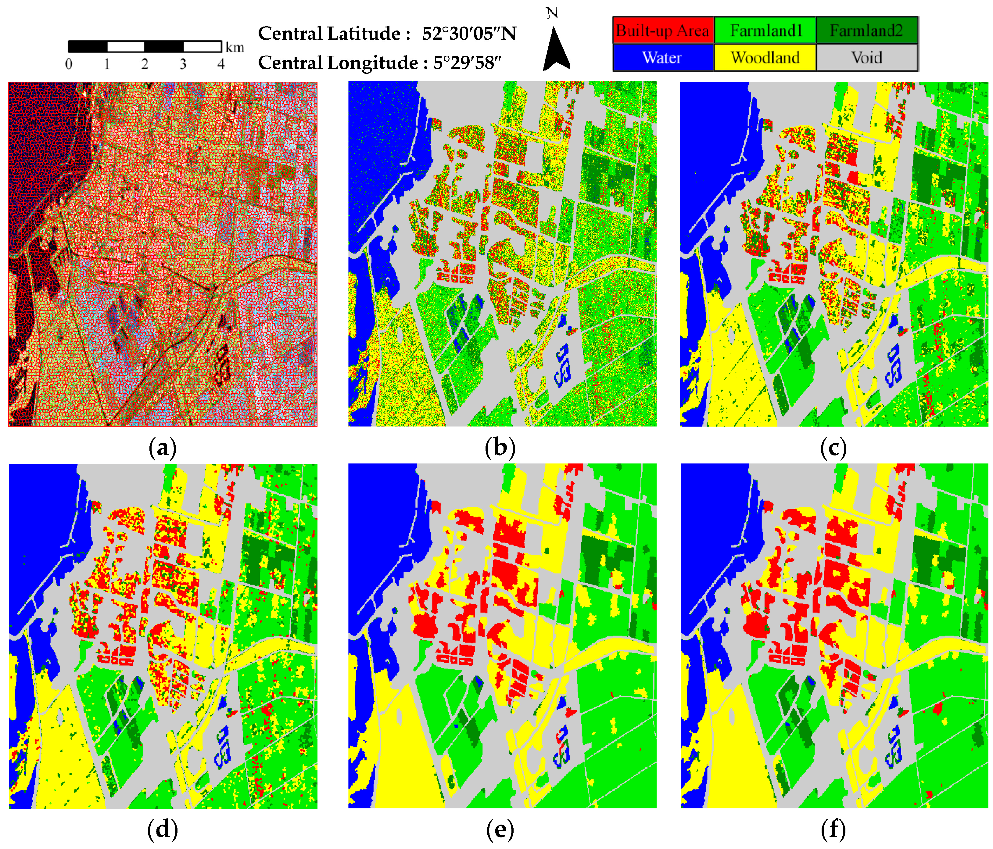
| Method | Water | Farmland | Woodland | Built-up Area | OA | Kappa |
|---|---|---|---|---|---|---|
| KSEM | 94.22 | 76.29 | 60.18 | 35.05 | 69.99 | 0.566 |
| KSEM-PLR | 98.46 | 89.18 | 88.06 | 50.69 | 85.07 | 0.785 |
| SP-KSEM | 96.67 | 85.02 | 90.47 | 55.10 | 84.13 | 0.775 |
| SP-WSEM-PLR | 97.45 | 93.54 | 98.15 | 61.43 | 90.65 | 0.867 |
| SP-KSEM-PLR | 95.61 | 97.03 | 97.65 | 71.54 | 93.16 | 0.902 |
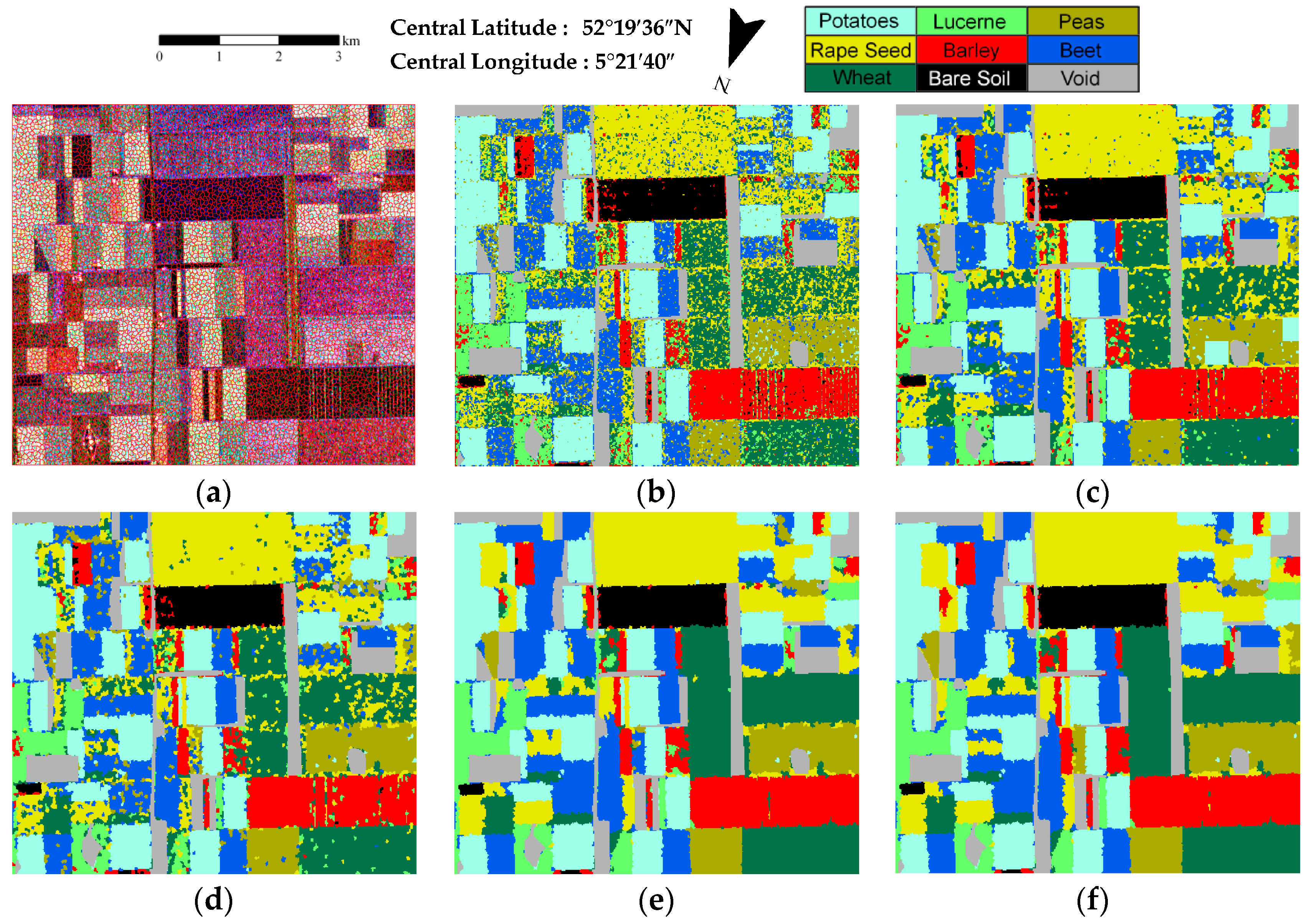
| Method | KSEM | KSEM-PLR | SP-KSEM | SP-WSEM-PLR | SP-KSEM-PLR |
|---|---|---|---|---|---|
| Potatoes | 90.93 | 94.00 | 94.31 | 95.86 | 95.83 |
| Lucerne | 76.63 | 83.88 | 83.04 | 93.74 | 94.51 |
| Peas | 65.93 | 64.91 | 78.62 | 82.20 | 88.64 |
| Rape Seed | 66.69 | 78.77 | 76.23 | 85.26 | 87.23 |
| Barely | 73.04 | 78.83 | 75.49 | 80.75 | 83.77 |
| Beet | 70.67 | 81.64 | 77.70 | 89.81 | 90.15 |
| Wheat | 66.41 | 76.73 | 78.52 | 87.42 | 87.28 |
| Bare Soil | 89.56 | 91.14 | 86.98 | 89.39 | 90.07 |
| OA | 74.52 | 81.85 | 81.55 | 88.45 | 89.70 |
| Kappa | 0.700 | 0.786 | 0.782 | 0.864 | 0.878 |
© 2016 by the authors; licensee MDPI, Basel, Switzerland. This article is an open access article distributed under the terms and conditions of the Creative Commons Attribution (CC-BY) license (http://creativecommons.org/licenses/by/4.0/).
Share and Cite
Xu, Q.; Chen, Q.; Yang, S.; Liu, X. Superpixel-Based Classification Using K Distribution and Spatial Context for Polarimetric SAR Images. Remote Sens. 2016, 8, 619. https://doi.org/10.3390/rs8080619
Xu Q, Chen Q, Yang S, Liu X. Superpixel-Based Classification Using K Distribution and Spatial Context for Polarimetric SAR Images. Remote Sensing. 2016; 8(8):619. https://doi.org/10.3390/rs8080619
Chicago/Turabian StyleXu, Qiao, Qihao Chen, Shuai Yang, and Xiuguo Liu. 2016. "Superpixel-Based Classification Using K Distribution and Spatial Context for Polarimetric SAR Images" Remote Sensing 8, no. 8: 619. https://doi.org/10.3390/rs8080619