Article

Airborne S-Band SAR for Forest Biophysical Retrieval in Temperate Mixed Forests of the UK

by Ramesh K. Ningthoujam 1,*, Heiko Balzter 1,2,†, Kevin Tansey 1,†, Keith Morrison 3, Sarah C.M. Johnson 1, France Gerard 4, Charles George 4, Yadvinder Malhi 5, Geoff Burbidge 6, Sam Doody 6, Nick Veck 7, Gary M. Llewellyn 8, Thomas Blythe 9, Pedro Rodriguez-Veiga 1,2, Sybrand Van Beijma 10, Bernard Spies 1, Chloe Barnes 1, Marc Padilla-Parellada 1, James E.M. Wheeler 1, Valentin Louis 1, Tom Potter 1, Alexander Edwards-Smith 3 and Jaime Polo Bermejo 11add Show full author list remove Hide full author list
1
Department of Geography, Centre for Landscape and Climate Research, University of Leicester, Leicester LE1 7RH, UK
2
National Centre for Earth Observation (NCEO), University of Leicester, Leicester LE1 7RH, UK
3
Radar Group, School of Cranfield Defence and Security, Cranfield University, Shrivenham, Swindon SN6 8LA, UK
4
Centre for Ecology & Hydrology, Wallingford OX10 8BB, UK
5
School of Geography and Environment, South Parks Road Oxford, University of Oxford, Oxford OX1 3QY, UK
6
Airbus Defence and Space—Space Systems, Anchorage Road, Portsmouth, Hampshire PO3 5PU, UK
7
Satellite Applications Catapult, Electron Building Fermi Avenue Harwell, Oxford Didcot, Oxfordshire OX11 0QR, UK
8
Natural Environment Research Council, Airborne Research & Survey Facility, Firfax Building, Meteor Business Park, Cheltenham Road East, Gloucester GL2 9QL, UK
9
Forestry Commission, Bristol and Savernake, Leigh Woods Office, Abbots Leigh Road, Bristol BS8 3QB, UK
10
Geo-Intelligence, Airbus Defence and Space, Compass House, 60 Priesley Road, Surrey Research Park, Guildford GU2 7AG, UK
11
Faculty of Civil Engineering and Geosciences Building, Delft University of Technology, 23 Stevinweg, Delft PO-box 5048, The Netherlands
*
Author to whom correspondence should be addressed.
These authors contributed equally to this work.
Remote Sens. 2016, 8(7), 609; https://doi.org/10.3390/rs8070609
Submission received: 19 April 2016 / Revised: 4 July 2016 / Accepted: 19 July 2016 / Published: 20 July 2016
(This article belongs to the Special Issue Remote Sensing of Vegetation Structure and Dynamics)

Abstract

:
Radar backscatter from forest canopies is related to forest cover, canopy structure and aboveground biomass (AGB). The S-band frequency (3.1–3.3 GHz) lies between the longer L-band (1–2 GHz) and the shorter C-band (5–6 GHz) and has been insufficiently studied for forest applications due to limited data availability. In anticipation of the British built NovaSAR-S satellite mission, this study evaluates the benefits of polarimetric S-band SAR for forest biophysical properties. To understand the scattering mechanisms in forest canopies at S-band the Michigan Microwave Canopy Scattering (MIMICS-I) radiative transfer model was used. S-band backscatter was found to have high sensitivity to the forest canopy characteristics across all polarisations and incidence angles. This sensitivity originates from ground/trunk interaction as the dominant scattering mechanism related to broadleaved species for co-polarised mode and specific incidence angles. The study was carried out in the temperate mixed forest at Savernake Forest and Wytham Woods in southern England, where airborne S-band SAR imagery and field data are available from the recent AirSAR campaign. Field data from the test sites revealed wide ranges of forest parameters, including average canopy height (6–23 m), diameter at breast-height (7–42 cm), basal area (0.2–56 m2/ha), stem density (20–350 trees/ha) and woody biomass density (31–520 t/ha). S-band backscatter-biomass relationships suggest increasing backscatter sensitivity to forest AGB with least error between 90.63 and 99.39 t/ha and coefficient of determination (r2) between 0.42 and 0.47 for the co-polarised channel at 0.25 ha resolution. The conclusion is that S-band SAR data such as from NovaSAR-S is suitable for monitoring forest aboveground biomass less than 100 t/ha at 25 m resolution in low to medium incidence angle range.

Graphical Abstract

1. Introduction

Forest is a living entity, capable of storing a large amount of carbon dioxide from the atmosphere. Terrestrial carbon is being stored in the form of aboveground biomass (AGB) as the trunk, branches and leaves of an individual tree, while forest AGB is the total biomass (living matter) of all growing trees per unit area. Quantification of forest AGB is essential to understand the spatial distribution of carbon in forests, particularly in old-growth forests [1] and to derive prognostics for monitoring the carbon stock trends.
Forest AGB is estimated with sample plot measurements from forest inventories e.g., in the tropics [2,3] and in Europe [4,5]. This approach of biomass measurement has been regarded as highly accurate; however, it involves some uncertainty primarily due to the use of allometric models to derive the forest AGB rather than direct measurements. Additionally, tree-level AGB estimates involve errors when upscaled to plot or landscape scale [6]. In the absence of large-scale inventory plots, most efforts for quantifying the distribution of biomass have focused on interpolation techniques at landscape or continental scale [7]. Due to the nature of the sampling with low temporal repeat frequency and a small number of inventory plots, the use of Earth Observation (EO) data acquired by satellite sensors are often being combined with field measurements [8,9,10]. For example, EO-based estimations have been shown to be similar to predictions derived from field estimates when averaging at large scales e.g., stand, landscape or even continental scale [11]. However, differences between biomass estimates are being reported particularly in regions with few sampling sites [12].
Wall-to-wall estimates of forest AGB derived from an integration of EO-data and field measurements across different biomes are available: tropical forest [9,10] and boreal forest [13]. For a long time, optical data with 8 km resolution from the Advanced Very High Resolution Radiometer (AVHRR) have been utilized. For example, forest AGB has been quantified over decadal periods across six countries (Canada, Finland, Norway, Russia, Sweden and the USA) with temperate and boreal forests from global AVHRR-derived maximum normalized difference vegetation index (NDVI) datasets [14,15]. The average absolute difference between EO-derived and inventory estimates was 27%, 33%, and 50% of the mean inventory estimates of AGB, total AGB and changes in carbon pools respectively. With the launch of the Terra and Aqua satellites carrying MODerate resolution Imaging Spectrometer (MODIS) instruments with spatial resolution down to 250 m, the bidirectional reflectance distribution function (BRDF) is also useful for mapping AGB across forests of different structures in Russia [16]. However, optical data are particularly sensitive to cloud cover, atmospheric aerosol loading and low solar illumination.
To overcome these limitations, advanced remote sensing technique of light detection and ranging (LiDAR) and microwave based Synthetic Aperture Radar (SAR) data are used. LiDAR data from the spaceborne Ice, Cloud and Land Elevation Satellite (ICESat) Geoscience Laser Altimeter System (GLAS) were utilized to estimate canopy height and estimates of AGB using empirically derived models that relate LiDAR variables to AGB using field plots with MODIS data [9,10]. The study by Saatchi, Harris, Brown, Lefsky, Mitchard, Salas, Zutta, Buermann, Lewis, Hagen, Petrova, White, Silman and Morel [9] has also utilized microwave data from QuickSCAT. Therefore, microwave based SAR sensors have been extensively used for forest characterization, mapping and assessing forest biomass because of the sensitivity of radar signals to complex forest structure and its component parts (trunks, branches and leaves) [17,18]. SAR satellites provide continuous data that are largely independent of cloud cover and solar illumination condition.
The first L-band observations at global scale were provided by the Japanese Earth Resources Satellite (JERS-1) SAR (1992–1998), while the Russian Almaz-1 (1991–1992) provided S-band and the Canadian RADARSAT C-band observations. X-band satellite missions, for example the COSMO SkyMed constellation and TerraSAR-X/Tandem-X were launched around mid-2000s by Italy and Germany respectively. Fully polarimetric observations at L- and C-band were provided by the Advanced Land Observing Satellite Phased Array L-band SAR (ALOS PALSAR, ALOS-2 PALSAR-2) and RADARSAT-2, ASAR or Sentinel-1 sensors respectively at a near global level. Renewed interest in S-band SAR has led to the launch of the Environment and Disaster Monitoring Satellite Huan Jing-1 Constellation (HJ-1C) by China [19] and new S-band SAR missions are planned, e.g., the UK NovaSAR S-band system [20] and the joint NASA-ISRO SAR (NISAR) missions [21].
The ability of the SAR signal to detect forest canopy components (trunks, branches and leaves) depends on its frequency, incidence angles and polarisations (HH, VV, HV or VH, with H and V representing the horizontal and vertical transmit/receive polarisation, respectively). The range of signal sensitivity to forest structure also depends on the canopy type (homogeneity to complex density) and environmental conditions (moisture content) [22]. The co-polarised channels (i.e., HH or VV) exhibit a large amount of scattered microwave energy with the strongest return at HH-polarisation due to double-bounce scattering from the vertical trunk structure lying perpendicular to the ground surface (unless in undulating terrain). In all forest types, microwaves emitted at longer SAR wavelengths (L- and P-band) are more sensitive to forest AGB due to deeper penetration and more interaction with the larger woody branches, trunks and ground surface, e.g., in boreal [23,24], temperate [25,26] and tropical forest [27]. This has been largely related to the cross-polarised channels (HV or VH) which have comparatively lower returns but generally increase asymptotically to the amount of woody biomass.
SAR signals at shorter wavelengths (C- and X-bands) are known to saturate rapidly with forest biomass due to lower canopy penetration. The microwave pulse primarily interacts with the foliage and smaller branches in the upper canopy layers at these wavelengths [28]. However, using high revisit C-band data from the Envisat’s Advanced Synthetic Aperture Radar (ASAR), Santoro, et al. [29] were able to estimate forest growing stock volume (GSV) using the BIOMASAR algorithm. On the basis of converting GSV to AGB using an expansion factor, wall-to-wall estimates of forest stock and carbon density have been generated over the temperate-boreal region of the northern hemisphere [13]. Further, sensitivities of forest biomass levels from multi-frequency SAR data (C-, L- and P-band) have also been reported from different forest types, e.g., coniferous (Les Landes and Duke) and broadleaved evergreen (Hawaii) achieving around 20 t/ha, 40 t/ha and 100 t/ha saturation levels respectively [30]. Vegetation optical depth (VOD) derived from passive microwave data is sensitive to high biomass density levels (e.g., in rainforests) [8]. Using the VOD data (1993–2012), an EO-based ABC (aboveground biomass carbon) estimation at global scale was produced for all vegetation types at >10 km resolution [8].
Amongst the different radar wavelengths, studies focusing on S-band data for forest structure and biomass characterisation have scarcely been investigated due to limited data availability. Almaz-1 S-band backscatter has been reported as having a very narrow dynamic range and similar average backscatter values in all the vegetation types [31] including palm and rubber plantations. Furthermore, Rosenqvist [31] questioned the effect of high incidence angle (~50°) to be the main factor responsible for this insignificant result in the Malaysian test site against the studies by Olsson, et al. [32] and Brown, et al. [33]. The sensitivity of S-band backscatter to forest structure and biophysical parameters has not been fully investigated.
This study assesses the sensitivity of S-band backscatter to forest biophysical parameters in a mixed temperate forest of the UK. Its main objective was to estimate forest structure (average tree diameter at breast height (DBH), canopy height (H)) and validate forest AGB from S-band backscatter data from 2010 and 2014 airborne acquisitions using field plot data at stand level. The Michigan Canopy Scattering (MIMICS-I) radiative transfer model [34] was used to understand the radiative scattering processes at S-band in forest canopies. The model simulations informed the parameter retrieval by explaining the physical basis for the retrievals.

2. Experimental Section

2.1. Site Description

For relating forest structure and AGB to S-band backscatter, the mixed temperate forest of Savernake Forest and Wytham Woods were chosen based on mixed species with varying levels of stand ages (10–262 years old), tree average DBH, canopy height, maximum canopy cover and AGB ranges. Additionally, maximum woody biomass is found between June and September in these forests where an airborne SAR data acquisition was available.
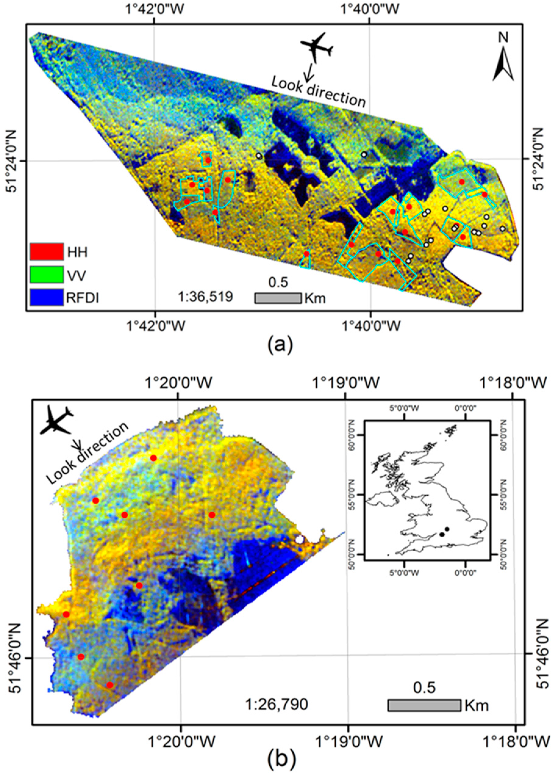
Savernake Forest (51°23’13”N, 1°43’19”W) is located near Marlborough in England, UK (Figure 1). The forest is composed of mixed stands of temperate deciduous and coniferous species with varying tree densities, canopy height, growing stock, and age class. Main deciduous species include ancient beech (Fagus sylvatica), birch (Betula pendula) and oak (Quercus spp.) with mixed species of yew, ash, common lime, crab apple, elm, field maple, hazel, horse chestnut. Dominant coniferous species consisted of Scots pine (Pinus sylvestris), Corsican pine (Pinus nigra), Norway spruce (Picea abies) and Western hemlock (Tsuga heterophylla).
The forest is managed by the Forestry Commission (FC) and composed of sub-compartments with an average size of 4 ha. Topography is relatively flat with an average elevation of 107 m and 1% slope with a south-eastern aspect [35]. The forest receives an average of 750 mm of annual precipitation and has an average annual temperature of 11.3 °C. Geologically, the parent soil material is characterized by Jurassic Clay (Oxford) with Eutric vertisol, has a soil pH of 3.9–6.2.
Wytham Woods (51°47’N, 1°20’W) is situated in the west of Oxfordshire in England, UK (Figure 1). The site represents a mixture of ancient semi-natural woodland, UK National Vegetation Classification community W8 Fraxinus excelsior-Acer campestre-Mercurialis perennis woodland [36] covering approximately 340 ha. The airborne data covers around 248 ha. The site has been continuously covered by trees [37] while recently managed with timber removal and plantation (e.g., beech, sycamore) where ash and sycamore species composition has been changed over time [38]. Since the last decade, it has become one of the most studied temperate deciduous woodland in the country related to Ash die-back disease [39], long-term monitoring plots for soil respiration [40], aboveground productivity, respiration and leaf production [41,42].

2.2. SAR Data and Processing

A number of SAR airborne campaigns have been undertaken in Europe [25,43] focusing on SAR bands at P-, L-, C- and X- frequencies. For the first time, an extensive S-band SAR campaign known as the ‘AirSAR Campaign’ has been conducted over the temperate region of the UK in 2010 and 2014. The Airborne SAR Demonstrator Facility ‘AirSAR’ is a collaborative project operated by Airbus Defence and Space (UK) with the Natural Environment Research Council (NERC) and the Satellite Applications Catapult [44].
SAR data was collected in the ‘AirSAR Campaign’ in 2010 and 2014. It consists of fully polarimetric intensity images at S-band (3.1–3.3 GHz). The acquisition and processing of SAR images was conducted by Airbus Defence and Space (UK). Details of the available SAR data from the different acquisitions dates used in this study and their characteristics are summarized in Table 1.
For the purpose of this study, pre-processing of S-band radar data includes antenna pattern correction, single look complex (SLC) to multi-look complex images with 5 × 5 kernel and speckle filtered using the Enhanced Frost filter. Geo-coding of the SAR imagery is done using an Ordnance Survey Master Map (Projection: United Kingdom, Datum: Ordnance Survey of Great Britain 1936) as reference with 30 (Savernake Forest) and 42 (Wytham Woods) widely distributed ground control points (GCPs), a second- order polynomial and nearest neighbour re-sampling to 3.75 m pixel size achieving a root mean square error (RMSE) of half a pixel. The radar backscatter coefficient was calculated using Equation (1) according to an Airbus technical report [45]:
σ° = 10 log10 (DN2)−Kcal
where: σ° = radar backscatter (dB), DN = pixel amplitude and Kcal = calibration constant. The calibration constants for Savernake Forest are 71.5 dB for HH and VH, and 71.47 dB for VV and HV polarisations for the image acquired on 16 June 2010, and 71.8 dB for HH, VH and 72.62 dB for VV and HV polarisations for the image acquired on 24 June 2014. The calibration constants for Wytham Woods are 81.46 dB for HH and VH and 81.9 dB for VV and HV polarisations for the image acquired on 23 June 2014. The ratio between HH- and HV-backscatter was utilized for classification of forest/non-forest maps [46]. It is known as the ‘Radar Forest Degradation Index’ (RFDI) because HH backscatter is sensitive to both volume and double-bounce scattering while HV backscatter is mostly sensitive to volume scattering from forest canopies [47].
For Savernake Forest, multi-temporal image calibration for the 2010 and 2014 data was performed using a correction factor of 7.16, 9.94 and 3.29 HH, VV and HV polarisations to 16 June 2010 data. The forest structure and biomass information content of S-band radar backscatter was examined at stand level by re-sampling the original 0.75 m to 25 m pixel resolution. The spatial aggregation is performed for each polarisation band using nearest neighbour resampling with the aid of a vector map (Ordnance Survey Master Map 1:25,000).

2.3. Field Data

For Savernake Forest, a total of 70 sample plots were collected with a circular sample area of 20 m diameter covering both deciduous and coniferous forest types. The first data set was collected in August 2012 and consisted of 38 sample plots distributed between young and mature stands giving a total of 19 sub-compartments. The field measurements include callipering of all trees on each plot with diameter at breast-height (DBH) ≥ 10 cm, canopy height (H) for a subset of the tallest trees and species identification of all trees for estimation of their wood density. Trunk diameter was estimated using diameter tape while canopy height was estimated using a combination of vertex hypsometer and a digital laser rangefinder (Nikon Laser600). Following the same field protocol, a second data set consisted of field measurements made during March 2015 after the second SAR campaign in June 2014. This relates to 32 sample plots with 16 sub-compartments covering the remaining compartments (Figure 1). The plot sites were located using a handheld differential GPS receiver.
For Wytham Woods, the Environmental Change Network (ECN) database is a spatially comprehensive database of tree species, tree diameter at breast-height (DBH) and canopy height (H) on the basis of [48] protocol covering over 10 m2 sample plots [49]. This corresponds to 8 sample plots from deciduous stands being collected by the Centre for Ecology and Hydrology research team in 2012.

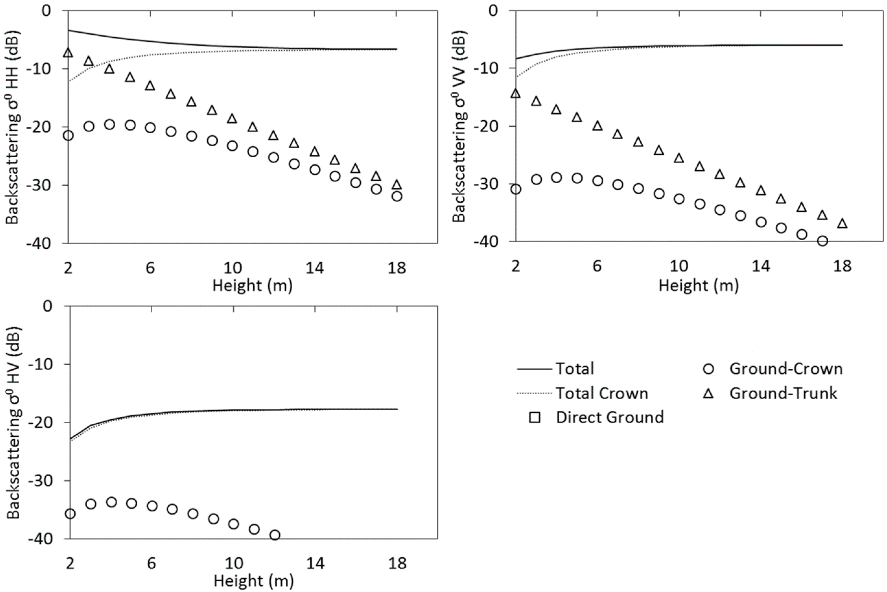
2.4. S-Band Radar Scattering Characteristics in Forest/Non-Forest Areas

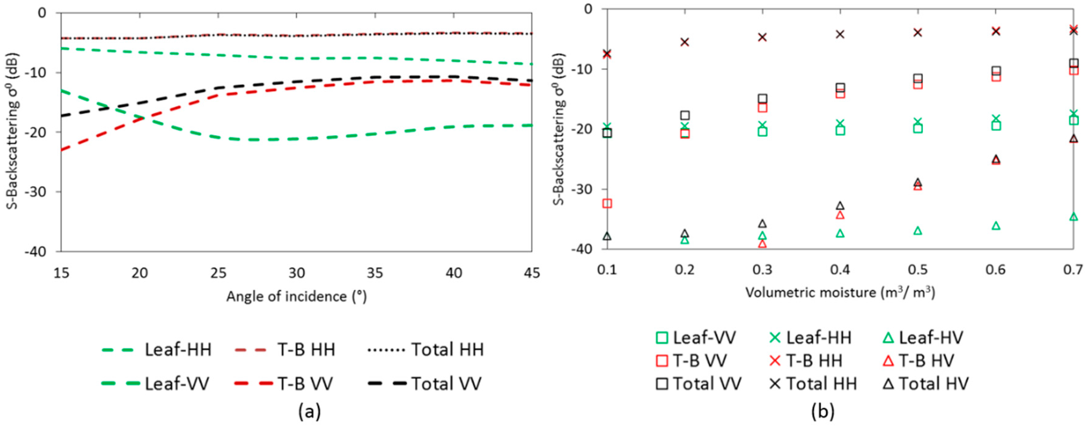
S-band backscatter and canopy transmissivity were simulated using the radiative transfer model Michigan Microwave Canopy Scattering (MIMICS-I) [34], a generic canopy structure driven forest canopy-based model designed to simulate radar backscatter based on canopy structure and first-order radiative transfer (RT) equations. MIMICS-I is a two-layer canopy model with upper canopy layer consisting of leaves, needles, branches and trunks as the lower layer which works on a first-order solution of the RT equations based on Foldy’s method (i.e., function of height within the canopy). Leaves related to deciduous species are modelled as flat rectangular discs while needles (conifer species) and branches are modelled as dielectric cylinders characterised by a joint probability distribution function (pdf). Trunks are represented by an average height and average diameter with their orientation being characterised by joint pdf while the ground surface as a function of soil types and roughness. All the components of canopy and ground are characterised by dielectric models in terms of moisture content, radar frequency and physical temperature.
A full description of MIMICS-I is given in [34] where details related to the input parameters for this study are given in Ningthoujam, et al. [46]. For relating to forest structure and identifying the dominant scattering mechanism purposes, the MIMICS model has been used to simulate multi-frequency (X-, C-, L-band) in a number of studies. For example, [50] assessed the sensitivity of C- and L-band backscatter over oak and pine species using MIMICS and model developed by Karam, et al. [51] across seasonal variations (summer against winter) in Fontainebleau forest, France. In the forest ecosystem of Queensland in Australia, the simulated backscatter using both MIMICS and multi-MIMICS were compared against the AIRSAR data [52]. MIMICS model simulations show that in the Brazilian Amazon, primary forest can be discriminated from regeneration and soil at L-band, but not at C-band due to deep penetration level in the canopy resulting to strong volume scattering [53]. Using MIMICS simulation, S-band backscatter shows sensitivity to the temporal dynamics of the structure of wheat crop [54].
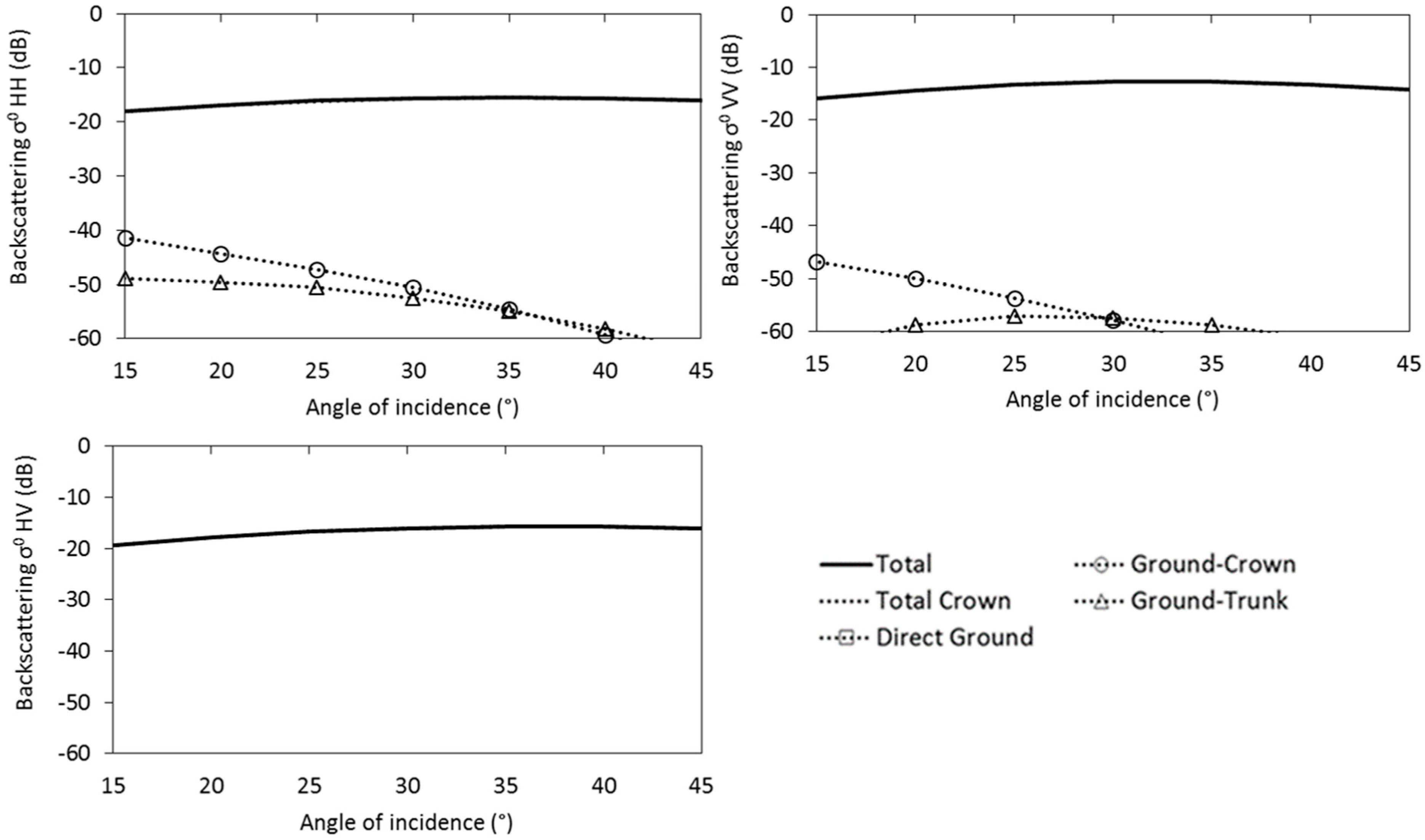
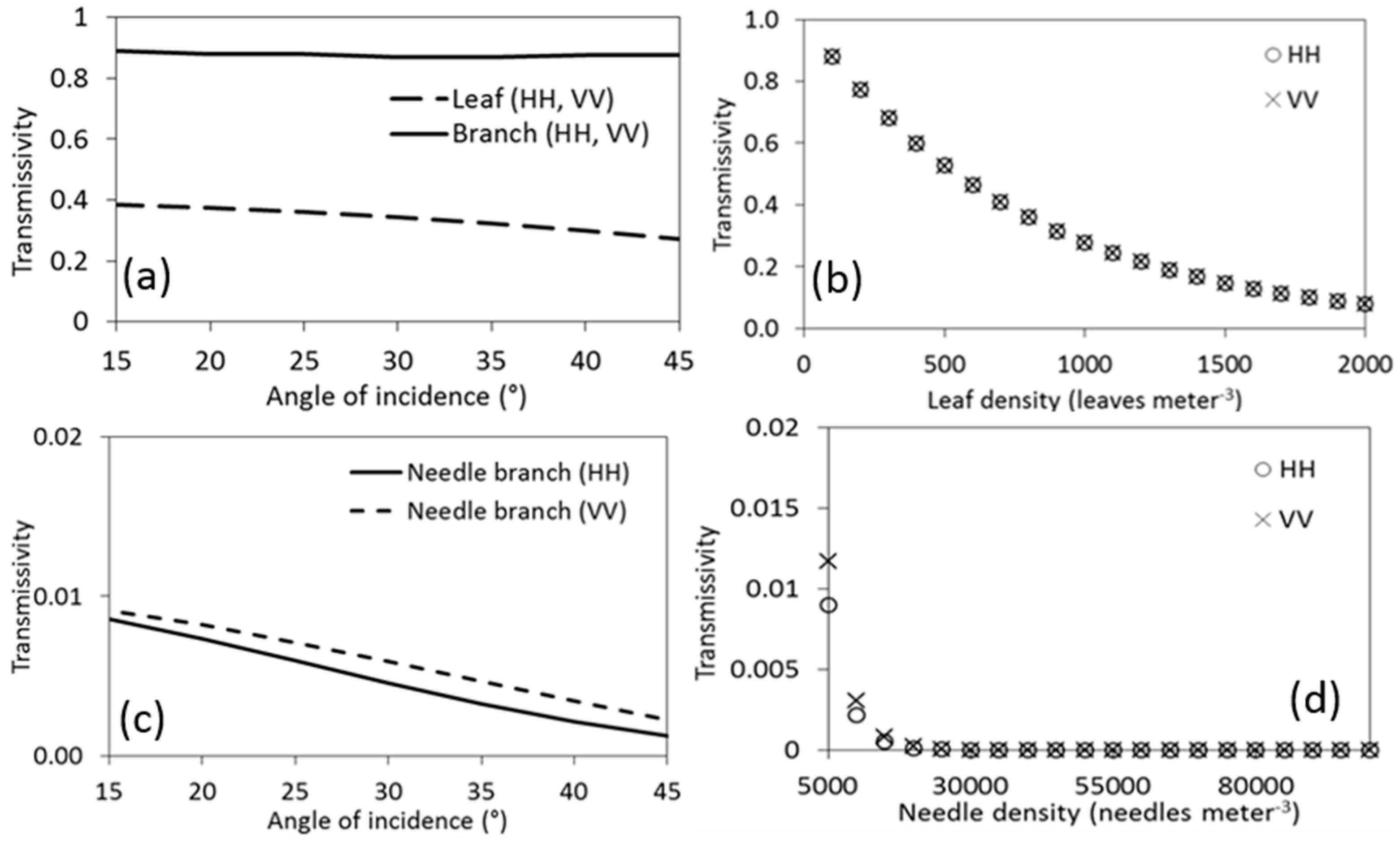
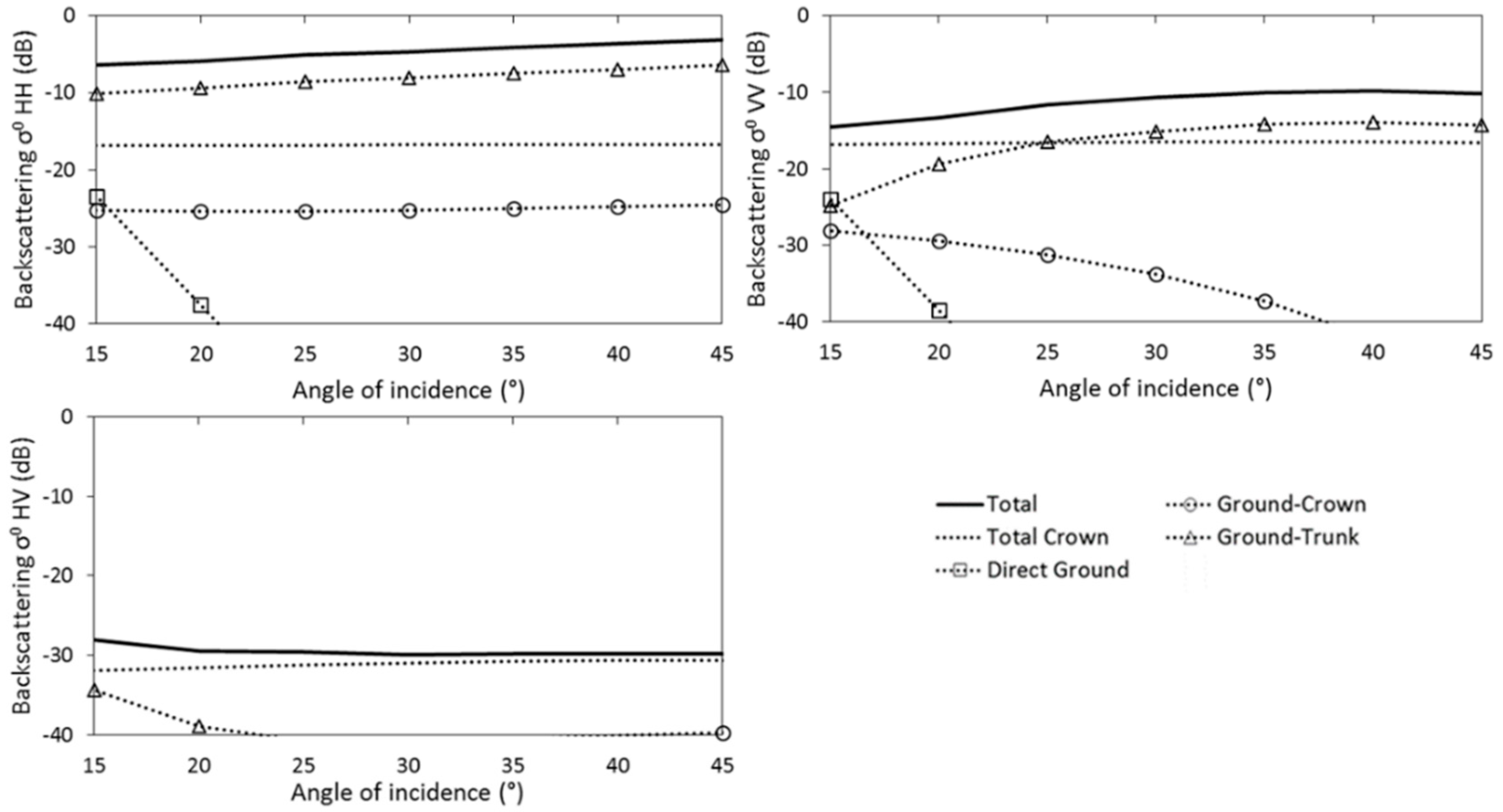
In this study, the sensitivity of S-band backscatter to forest canopy parameters and its components is investigated as a function of canopy types, canopy density, stand height and varying moisture content and SAR system parameters (multi-polarisation, incidence angles). Specifically, the radar frequency range at 3.1 GHz (15 cm) with incidence angles between 15°–45° were used. The canopy transmissivity and contribution of the individual interactions to the total canopy backscatter at S-band are reported here. Radar canopy transmissivity is related to the power transmission coefficient for propagation from the forest component at a specified incidence angle while backscatter is the overall scattering returns (attenuation) back to sensor (receiver) from forest canopy in a pixel resolution cell.

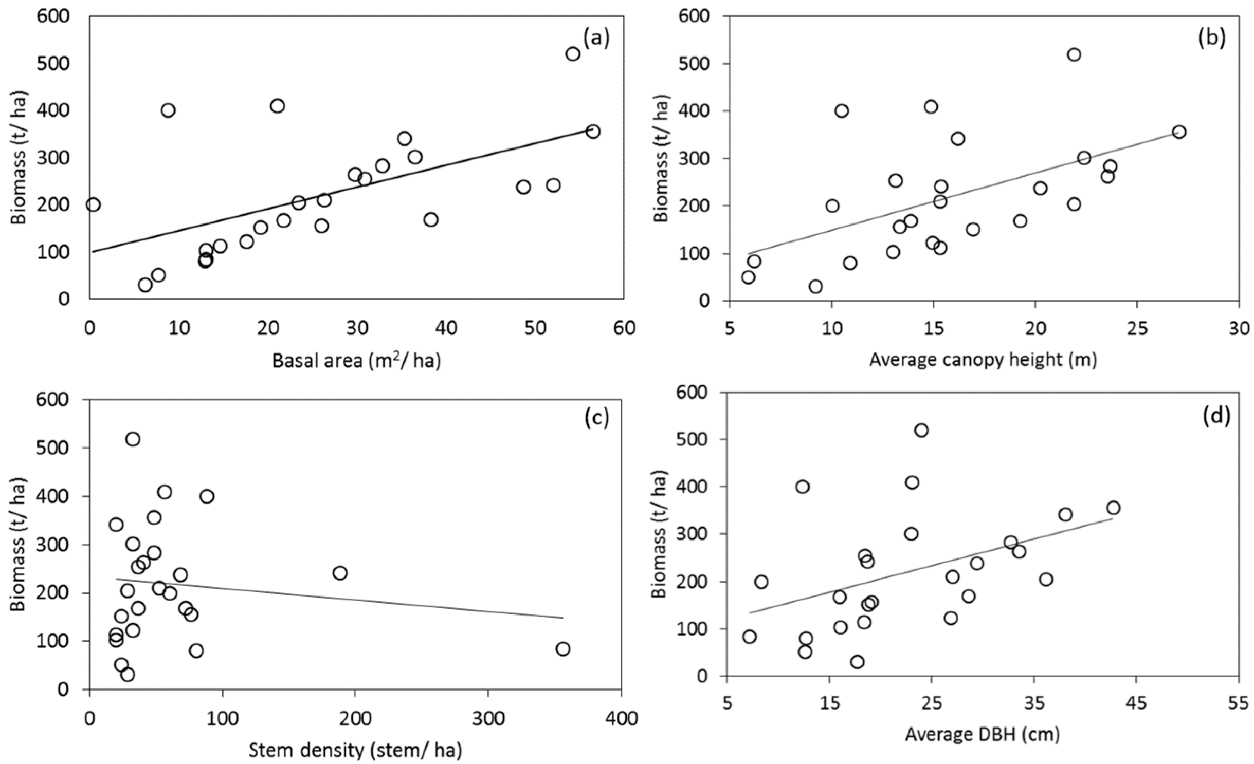
2.5. S-Band SAR Backscatter Relationships with Forest Structure and Biomass

At the individual tree-level, the AGB was estimated using the allometric equations reported in [55,56] which were specific to British tree species (including European genera) and tree size measurements as inputs for Savernake and Wytham. The allometric equations for different species used in this analysis are given in 
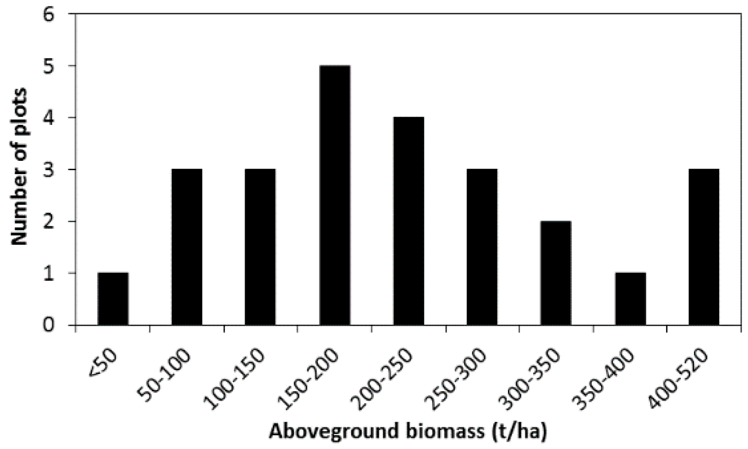
Table 2. From the tree-level estimates of AGB, plot level estimates of biomass were obtained by the summation of single tree AGB in each plot. Finally, the estimated AGB is measured in units of metric tonnes per hectare (t/ha) for statistical comparison with S-band backscatter.
Of the total 19 sub-compartments in Savernake, 2 sub-compartments were discarded in the analysis. First, 1 sub-compartment was located at the very edge of the SAR imagery (near to 15° incidence angle range) having erroneous values caused by the re-sampling method. The second sub-compartment was discarded due to large diameter trees ≥70 cm resulting in an AGB much larger than 700 t/ha.
The backscatter response from a forest stand is a combination of different sources, e.g., forest parameters, layover of tree canopy, speckle, geolocation errors and border effects including moisture content. Although the impacts of these factors are difficult to quantify, studies have shown the role of spatial resolution as an important factor in understanding the spatial variability of forest structure and AGB [23,27]. Since the field sample plot size of 10 m × 10 m and 20 m diameter for Wytham Woods and Savernake Forest appears too small for a useful comparison with the SAR data, the backscatter estimates were aggregated to stand level. The extent of each stand was defined based on the FC sub-compartment polygon for Savernake Forest. However, based on the available sample plot size and for the purpose of this study, stand level analysis at 0.25 ha and 0.5 ha corresponding to 25 m and 50 m pixel resolutions were considered and 0.25 ha selected as a minimum stand size.
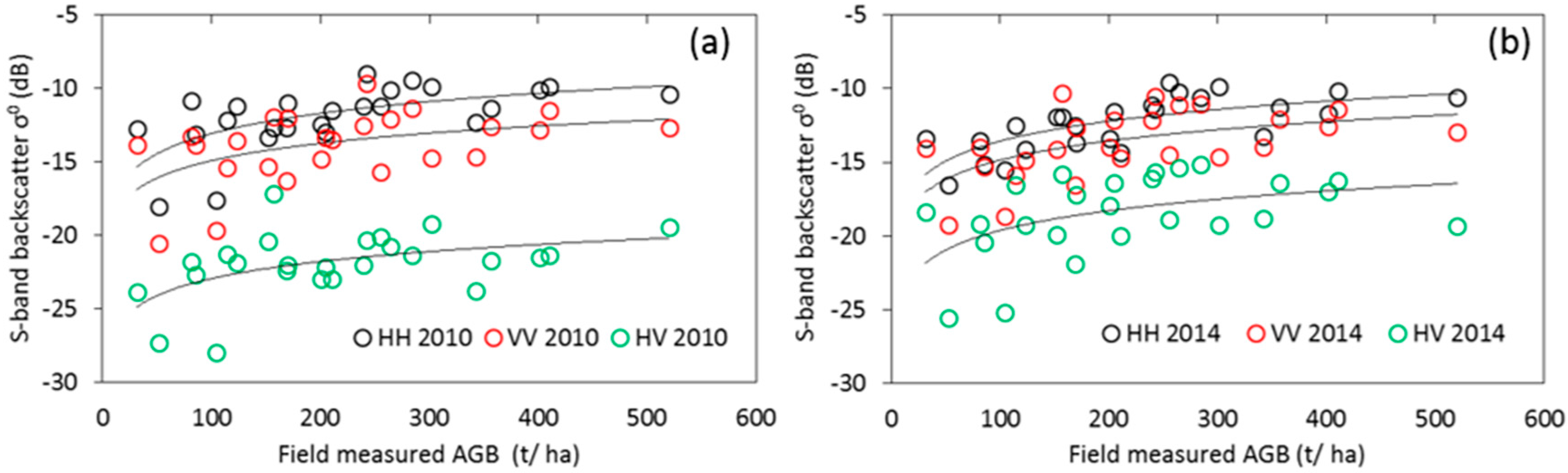
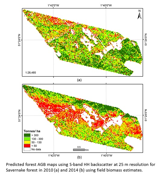
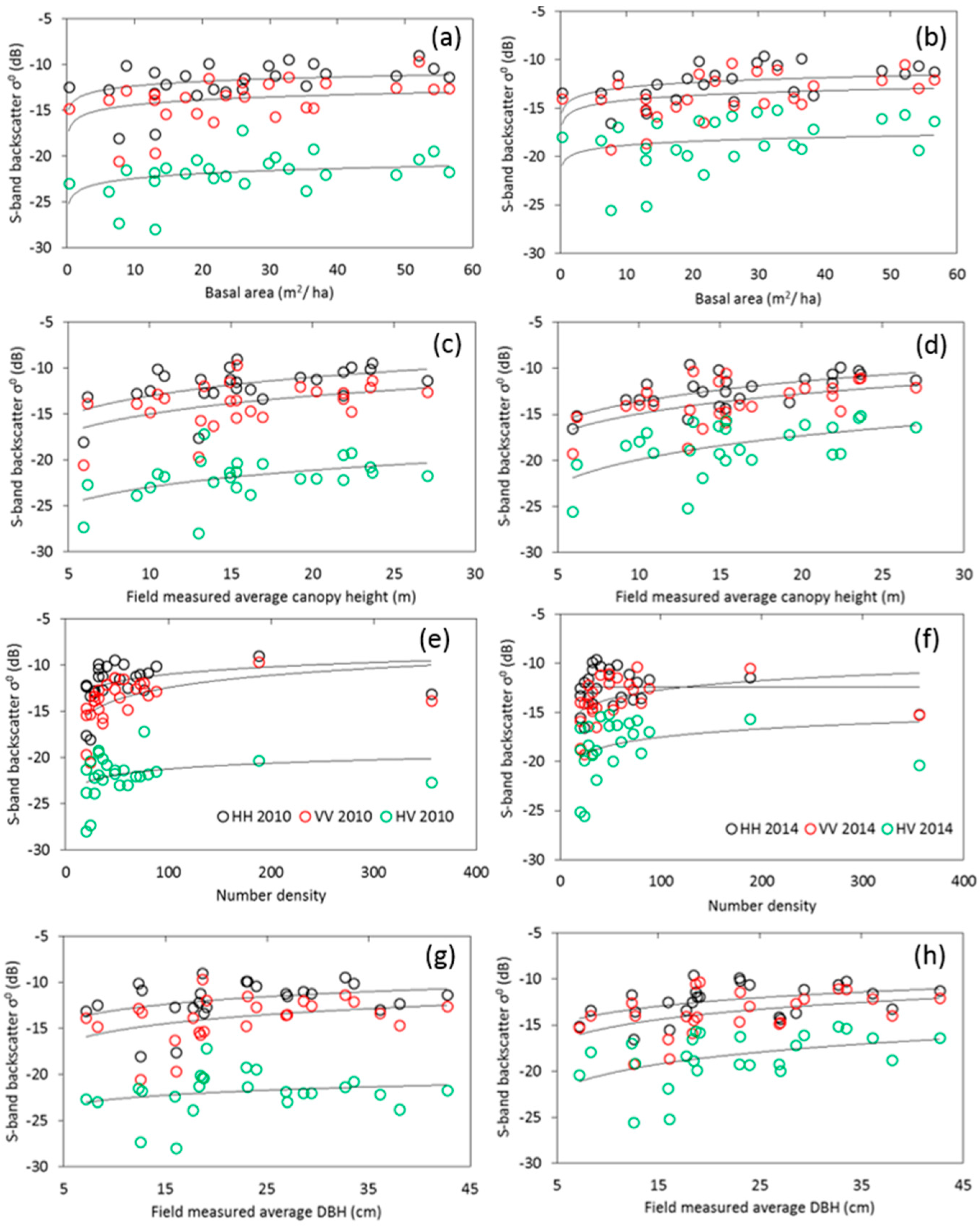
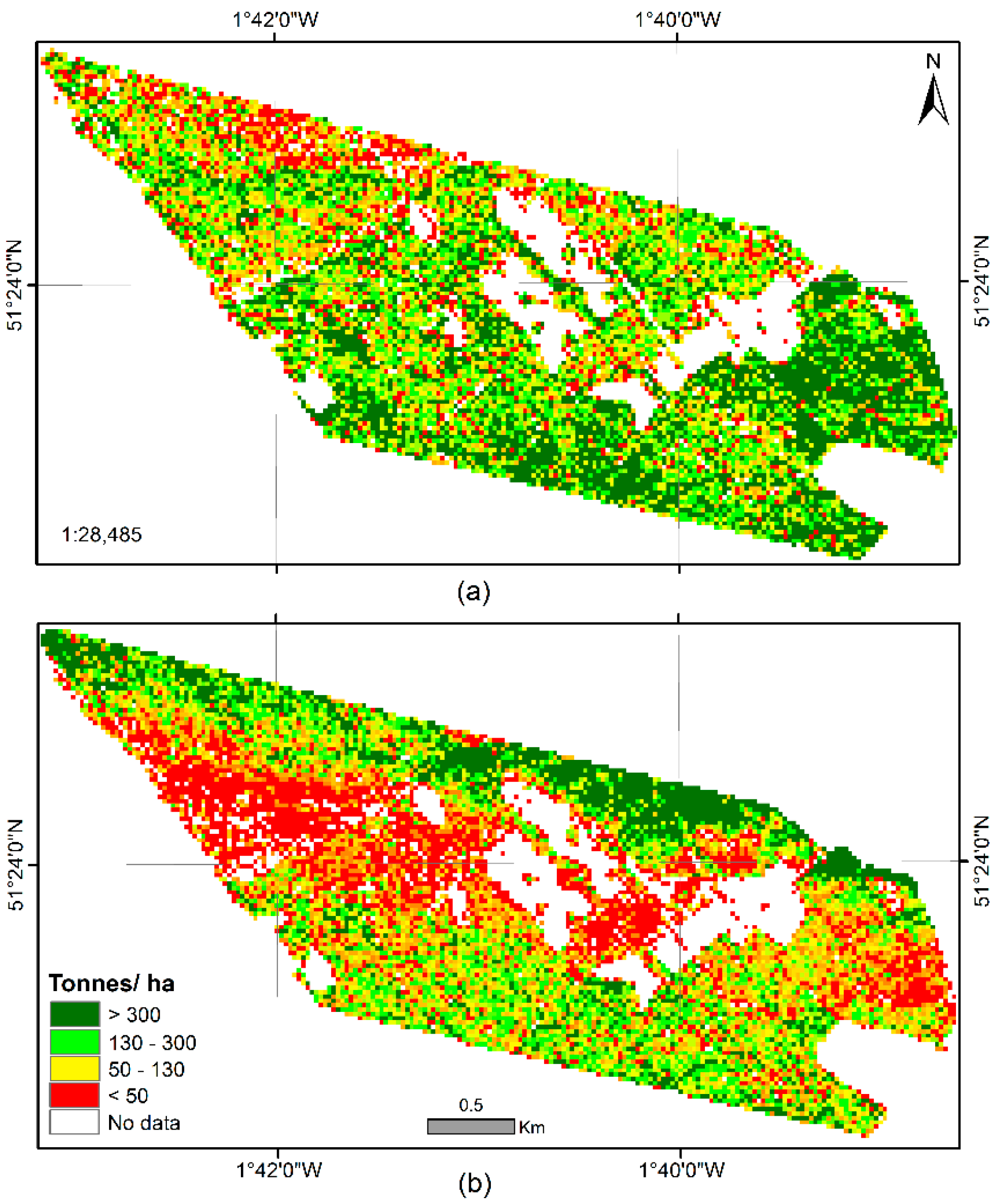
The fully polarimetric S-band backscatter were regressed against plot-measured AGB at stand (0.25 ha and 0.5 ha) levels utilising 25 sample plots. This was done using SAR data acquired on 16 June 2010, 23 and 24 June 2014 in Wytham and Savernake sites. The corresponding forest stands with 17 (9 deciduous, 8 conifer) and 8 (deciduous) plots from Savernake and Wytham Woods respectively were used to develop a regression model describing the relationship between AGB and S-band backscatter, referred to as training plots. Quantification of the S-band signal saturation level to field calculated AGB was also performed. Furthermore, using the best logarithmic model, prediction of AGB at 0.25 ha was produced. The second data set consisted of field measurements made during April 2015 in Savernake. These 16 forest stands (10 deciduous, 6 conifers) were used to validate the developed biomass regression models, referred to as validation plots. This includes biomass error estimation based on RMSE calculated by comparing model prediction to field measured AGB using model training (25) and validation (16) plots.

3. Results

3.1. Field Data

The average tree DBH and canopy height related to field measured plots for Savernake are 20.35 cm and 17.0 m respectively. Wytham Woods yielded average tree DBH and canopy height around 24.47 cm and 15.0 m respectively. Based on a total of 17 plots obtained in 2012, Savernake Forest yielded a minimum, average and maximum AGB of ~31.4 t/ha, 223.8 t/ha and 410 t/ha respectively. On the other hand, a minimum, average and maximum AGB of ~52.1 t/ha, 208.59 t/ha and 520.1 t/ha were recorded based on 8 sample plots from the Wytham site. When the biomass information for both sites was combined, an average AGB value of 218.9 t/ha was observed. The second data set for Savernake Forest related to 16 sub-compartments, yielded a minimum, average and maximum AGB of ~32.9 t/ha, 228.7 t/ha and 469.3 t/ha respectively.
Figure 2 shows total number of plots (n = 25) with varying levels of biomass (31.4–520.1 t/ha) used to relate plot measured AGB against S-band backscatter for both the sites. The SAR data acquired in both June 2010 and 2014 for Savernake and 2014 for the Wytham sites at stand levels were analysed.
The calculated aboveground biomass values were significantly related to basal area and average canopy height in comparison to stem number density and average DBH of the plots (Figure 3 and Table 3). The relationships of biomass to basal area and average canopy height produced an r2 = 0.34 and r2 = 0.3 (p < 0.005) (linear model). However, a weaker correlation between biomass and the average DBH for each plot when a linear model was observed (r2 = 0.18, p < 0.05). The poor distribution of stem densities also compromises the poor correlation with forest biomass.

3.2. MIMICS-I Model Simulation Experiment

The simulated canopy transmissivity for broadleaved birch canopy reveals medium (0.4) to high (0.9) transmissivity values at S-band frequency in leaf-dominated and branch-dominated experiments for both HH- and VV-polarisations. The transmissivity values decreases across the incidence angle range with high scattering from ground/trunk interactions from the branch-dominated canopy (Figure 4a). The transmissivity value also decreases with increasing leaf density in both polarisations at average incidence angle ~30° (Figure 4b).
In the Norway spruce canopy, simulations gave very low canopy transmissivities (below 0.1) for both polarisations across the incidence angle range (Figure 4c). This small value of canopy transmissivity is due to the high density of needles (85,000) and 3.4 branches used to model the canopy with 11 meter crown layer thickness. Moreover, the transmissivity also drastically decreases with increasing needle density in both polarisations (Figure 4d).
The simulated S-band backscatter from the forest canopy is a function of dielectric constants of different canopy parts in terms of moisture content. At S-band, backscatter signals from leaves decrease across the radar incidence range as a function of moisture content, with lower sensitivity (logarithmic model: r2 = 0.7, p < 0.0001) for HH- (RMSE = 0.46), (logarithmic model: r2 = 0.69, p < 0.0001) for VV- (RMSE = 0.47) and (logarithmic model: r2 = 0.57, p < 0.0001) for HV- (RMSE = 0.92) polarisations at 0.5 volumetric moisture content, details can be found in Figure A1. Backscattering from trunk/branch increases across the radar incidence range as a function of moisture content with high sensitivity. A similar pattern is also evident for total backscatter from the canopy (Figure A1). With varying moisture content between 0.1 and 0.7 m3/m3 in different canopy parts, S-band radar backscatter also shows significant sensitivity to branch and trunk components (logarithmic model: r2 = 0.95) for HH- (RMSE = 0.29), (logarithmic model: r2 = 0.98, p < 0.0001) for VV- (RMSE = 0.49) and (logarithmic model: r2 = 0.78, p < 0.0001) for HV- (RMSE = 3.25) polarisations at average incidence angle of 30° (Figure A1).
For a broadleaved birch canopy, simulated S-band radar total backscatter originates from ground/trunk interaction in HH-polarisation while scattering from VV-polarisation is a combination of total crown (direct) and ground/trunk components across the radar incidence range (see Figure 5). In the case of cross-polarisation, total crown (direct) exerts the main dominating factor to the radar total backscatter. This could be due to the reduced transmittance as a function of increasing leaf and branch density. In all the polarisations, backscatter from direct ground (a function of soil moisture and roughness) is lower across the incidence angle range than forest canopy backscatter, possibly due to single scattering from the terrain surface. Additionally, the depth of crown and density of leaves/branches played a significant role in the strength of the backscatter signal.
For Norway spruce canopy, simulated S-band radar total backscatter is lower than for a broadleaved canopy, being dominated by the total crown (direct) component across the incidence angle range for both co- and cross-polarisations. The details of this relationship can be found in Figure A2. This is due to the lower volume scattering [57], as the main scattering originates from the needles and branches of conifers [58]. Figure 6 shows the simulated S-band radar total backscatter at average incidence angle ~30° for increasing birch canopy height at HH-, VV- and HV-polarisations. At S-band, dominant backscatter comes from the ground/trunk interaction up to 5 m stand height (in the case of HH-polarisation) while maximum scattering comes from the crown layer (direct crown) with increasing stand height in all polarisations.

3.3. S-Band Backscatter Sensitivity to Forest Structure

Different logarithmic relationships were found between S-band backscatter and basal area, average canopy height, stand density and average diameter at breast height (Figure 7). For basal area, a weaker logarithmic relationship was found with S-band σ° backscatter at 0.25 ha for both years with highest in the HH polarisation (Table 4). There was a significant response to average canopy height in HH polarisation for both years (r2 = 0.28 for 2010, p < 0.05 and r2 = 0.45 for 2014, p < 0.0005) (Table 5). This sensitivity appeared to occur quite early in both years up to about 9–10 meter height as the saturation level to S-band backscatter. A weaker relationship was found with stem density in all the polarisations except VV polarisation for 2010 data (VV: r2 = 0.3 for 2010, p < 0.1) (Table 6). Similarly, a weaker and insignificant relationship was found between average DBH for the plot and all polarisations (Table 7).

3.4. S-Band Backscatter Sensitivity to Forest Aboveground Biomass

The relationship of S-band polarimetry from 16 June 2010, 23 and 24 June 2014 are plotted against plot AGB (Figure 8). Both co- and cross- polarised backscatter is highly dependent on AGB and shows better sensitivity to forest biomass at stand level for both years in both sites. For both forest sites, lower dynamic range of backscatter (around 8 dB) was observed in both 2014, whereas a slightly higher dynamic backscatter range (around 10 dB) for all polarisations was observed for 2010 data. S-band backscatter increases with biomass up to some levels around 100 t/ha in all polarisations, after which no further sensitivity is observed. This trend is easily evident in 2014 data in comparison to 2010 data. For instance, HH polarised backscatter acquired in 2014 produces the highest sensitivity to AGB with r2 = 0.5 (RMSE = 1.34, p < 0.0001) while r2 = 0.37 (RMSE = 1.75, p < 0.005) in 2010 for both forest sites (Table 8).
VV polarised backscatter acquired in 2014 shows medium sensitivity to AGB with r2 = 0.3 (RMSE = 1.94, p < 0.005) while r2 = 0.22 (RMSE = 2.17, p < 0.05) in 2010 data for the study sites (Table 8). Finally, the 2014 acquired HV polarised backscatter produces the lowest sensitivity to AGB with r2 = 0.22 (RMSE = 2.46, p < 0.05) while r2 = 0.24 (RMSE = 2.01, p < 0.05) in 2010 data (Table 8).

3.5. Estimation of Forest Aboveground Biomass Using S-Band Backscatter

The logarithmic model was used for relating plot AGB to S-band backscatter co-efficient as
σ° (dB) = Constant + Slope × ln (AGB) (t/ha)
For further analysis, the AGB was predicted based on S-band radar backscatter acquired on 16 June 2010 and 23 and 24 June 2014 at 0.25 ha resolution for both sites as input. For both forest sites, the predicted AGB based on 2010 data ranges from 18.75 to 978.67 t/ha, 4.34 to 1038.98 t/ha and 23.34 to 796.71 t/ha for HH, VV and HV polarisations respectively. Additionally, AGB was predicted ranging between 22.19 to 772.88 t/ha, 10 to 761.48 t/ha and 5.67 to 914.7 t/ha for HH, VV and HV polarisations respectively for the 2014 data (Figure 9). For Savernake Forest, the S-band has identified aboveground biomass with the majority of biomass up to 300 t/ha (Figure 9 for HH-backscatter). This is more evident in 2010- derived than 2014 -derived based biomass predictions.
Biomass predictions for the 2014 data had biomass >300 t/ha and reaching up to 550 t/ha particularly in conifer stands. This may be possible as the conifers in these sub-compartments are aged between 20 and 75 years old with high biomass content. However, there are distinct differences in some areas between the maps and field estimates. Comparing both the biomass maps and field data, it seems that predicted biomass for 2010 data is under-estimated for high biomass stands particularly in conifer compartments while over-estimated for low biomass stands in the case of 2014 data. Both these errors (over- and under-estimations) are primarily confined to those areas where field data is largely lacking and the actual biomass has not been well captured by the S-band radar derived model.

3.6. Accuracy of S-Band Backscatter-Biomass Regression

The relationship between AGB recorded by field observations and those predicted by the linear regression model for 0.25 ha resolution in different polarisations for both years over Savernake Forest performed well for low biomass level stands, but most of the stands having high biomass are either under- (HH polarised) or over-estimated (VV and HV polarised). For the model training plots, forest AGB predicted at 25 m resolution for 2014 was better than 2010 predictions. For instance, HH polarisation produced RMSE of 90.63 t/ha while HV polarisation produced a larger error of 114 t/ha. On the other hand, forest AGB predictions for 2010 produces relatively larger RMSE variations between 99.39 to 119.03 t/ha in all polarisations (Table 9).
For the validation plots in Savernake Forest, the errors were larger. For instance, VV polarisation displayed the lowest RMSE of 97.91 and 107.8 t/ha for 2010 and 2014 with highest correlation r2 = 0.47 and 0.35, respectively. HH polarisation produced RMSE of 108.4 and 114.23 t/ha with correlation r2 = 0.35 and 0.27 respectively. Similarly, larger error ranges varied between 97.91 to 129.91 t/ha was predicted by the model for all polarisations with varying weak to good relationships (Table 9). Comparing all polarisations, it is seen that S-band co-polarised backscatter data is better suited for biomass estimation than the cross-polarisation backscatter.
Figure 10 shows the cross-comparison of forest biomass predicted using S-band backscatter between 2010 and 2014. S-band predicted forest biomass between 2010 and 2014 has shown some relationship. VV polarised predicted forest biomass has the strongest agreement while the weakest relationship in the case of HV polarisation. This is due to the highest error associated with HV polarisation (Table 9). For all the polarisations, higher sensitivity between 2010 and 2014 predicted forest biomass is found below 150 t/ha in comparison to higher biomass stands.

4. Discussion

4.1. Modelling Simulation

MIMICS-1 model simulations suggests that S-band radar backscatter interacts with different canopy components particularly with large branch, trunk and ground layer depending on the canopy type and structure and provides some information related to forest structure. For broadleaved birch canopies, simulated total S-band radar backscatter originates from ground/trunk interaction in co-polarisation while total crown scattering (direct) exerts the main dominating factor to the total radar backscatter in the case of cross-polarisation. This could be due to the reduced transmittance as a function of increasing leaf and branch density. The depth of crown and density of leaves/branches has a significant role in the strength of the backscatter signal.
For coniferous stands, simulated total S-band radar backscatter is lower than for a broadleaved canopy, being dominated by the total crown (direct) component across the incidence angle range for both co- and cross-polarisations. This demonstrates that the S-band radar signal is unsuitable for penetration within the conifer canopy, possibly due to the randomised diffuse scattering from needles and small branches [58] and hence lower volume scattering [57]. The simulated S-band backscatter from the forest canopy has also shown significant sensitivity to moisture content of different canopy parts particularly branch and trunk components across the radar incidence range. A similar pattern is also evident for total backscatter from the canopy.

4.2. Sensitivity of Forest Structure and Aboveground Biomass to S-Band Backscatter

Experimental S-band radar data were observed to have varying sensitivity to field-estimated basal area, average canopy height and average tree diameter for all polarisation at 0.25 ha resolution. For all the forest structural properties, a weaker relationship with S-band backscatter was found. In comparison to the forest properties, the S-band radar backscatter provides a consistent sensitivity over forest AGB at 0.25 ha resolution. Hence, at the stand level analysis with 25 m resolution, S-band backscatter had a positive relationship with forest AGB, particularly in co-polarised HH- (r2 between 0.37 and 0.5) and VV- (r2 between 0.22 and 0.3). This relationship between S-band backscatter and biomass could be due to averaging a larger number of pixels with reduced speckle noise. Studies in tropical rainforest of La Selva (Costa Rica) have observed plot sizes at least with 0.25 ha to be sufficient to achieve normal distribution of basal area and biomass over forest landscape [27,59]. However, for this study the accuracy of the spatial averages of backscatter to biomass relationship is reduced if the area size is beyond 0.25 ha. This reduced relationship when up scaled up to 0.5 ha stand plot size may be due to lack of field data greater than 0.25 ha or no longer sufficient enough to derive the underlying forest biophysical information against the average backscatter returns.
Both the forest biomass maps related to 2010 and 2014 data revealed a general agreement for the sites with biomass ≤150 t/ha which S-band radar backscatter seemed to be sensitive. Large differences in AGB predictions between 2010 and 2014 may be due to imperfect radiometric calibration, varying incidence angles between the SAR imageries and field data acquired in 2012 and 2015 resulting in different biomass allometric models for both SAR datasets. The relationship between AGB recorded by field observations and those predicted by the linear regression model for 0.25 ha resolution in different polarisations for both years over Savernake Forest performed well for low biomass level stands ≤150 t/ha for both training and validation plots. Comparing all polarisations, it is seen that S-band co-polarised backscatter data is better suited for biomass estimation than the cross-polarisation backscatter.

4.3. Uncertainty Analysis

There are three major sources of uncertainty in this study: uncertainties in calculating backscatter values from MIMICS model simulation, field data including allometric equations and biomass estimation using the S-band radar signal.
Uncertainty related to the MIMICS-I model simulation includes the use of published values for the number of leaves, needles and branch densities and their spatial orientation which are adopted due to the difficulty in measuring these in the field. Moreover, the MIMICS-I model works with a single even-aged or mono-species canopy which does not account for forest stands of mixed species composition and structure with multiple canopy layers. Therefore, it is likely that some uncertainty will be found in the model-derived backscatter due to the lack of ground information and model limitation.
The uncertainty in field data measurement and AGB estimation from tree diameter measurements are considered very accurate in comparison to height measurements. Measurements of tree height using a hypsometer in 2012 and digital laser rangefinder in 2015 suggested that our methods may introduce some error. Since the species diversity in both study sites was very low, mis-identifications are likely to be relatively few, and given the similarities of wood density within a genus are unlikely to have a major effect on the biomass estimation [2,60]. Generally, biomass is estimated using DBH as the main variable in the allometric models [3]. Chave, et al. [2] demonstrated a higher accuracy of the allometric models by combining the tree DBH with stand height information. Other sources of errors in estimating the forest stand biomass could be related to the spatial variability in forest structure and the lack of sampling of small trees with DBH < 10 cm. This can potentially introduce bias hence influencing the accuracy of the field biomass estimates. However, this study has used the allometric equations of Bunce [56] and Zianis, Muukkonen, Mäkipää and Mencuccini [55] which were specific to British tree species rather than direct field estimation through tree harvesting and can potentially introduce errors [6,18]. Therefore, biomass retrieval using S-band radar backscatter can also incur uncertainty due to the limited number of field sample plots particularly in stands with low tree density and trees with DBH < 10 cm. Uncertainties related to differences in biomass estimation from the S-band radar signal between 2010 and 2014 could be due to varying incidence angles resulting in possible calibration errors between the SAR images. Future research for assessing the temporal biomass change in Savernake Forest would provide further insights into temporal aspects.
This study utilises SAR data acquired at 16°–44° radar incidence angle range which falls within the range of 38°–44° reported by Brown, et al. [33] and highlighted some relationship with biomass, unlike other studies [31,32]. Hence, the sensitivity of S-band radar backscatter to forest biophysical characteristics can be confirmed similar to Brown, et al. [33], to an extent where sensor look angle could play a significant role in detecting stand characteristics acquired at 16°–44° radar incidence angle range.

5. Conclusions

A wide consensus for increasing backscatter in low biomass values and subsequently insensitivity at higher biomass values has been reported for different radar wavelengths particularly at low-frequencies [17,23,25,26,27,30]. For this study, the modelling simulation at S-band is useful for the retrieval of forest canopy structure. The HH- and VV-polarisations were found to be optimal for forest structural retrieval for deciduous species because of the strong signal originating from ground/trunk interactions. S-band radar backscatter can be linked to biomass provided the relationships between biomass elements in different components of the tree are known. However, a weak relationship is found between S-band radar backscatter and mean canopy height and canopy structure of conifers, possibly due to the high density of needles and branches.
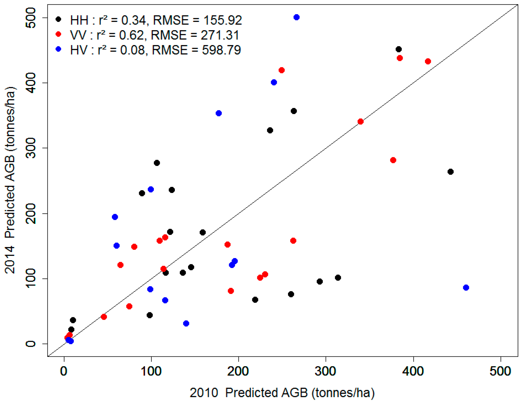
Experimental S-band radar data was observed to have varying sensitivity to field-estimated forest properties. Forest AGB shows sensitivity with S-band backscatter particularly for co-polarisations at 25 m resolution (stand level). The relationship of S-band backscatter with forest stands up to 300 t/ha biomass has shown the lowest error between 90.63 and 99.39 t/ha. S-band backscatter can be used to retrieve AGB in low biomass forests with lower errors in temperate forest with mixed deciduous species, particularly at low to medium incidence angles. Due to the varying incidence angles and possible calibration errors between the SAR images, the uncertainty related to large differences in biomass estimation from the S-band radar signal between 2010 and 2014 could not be accounted for. Although these results indicate a considerable potential for retrieval of forest structure and aboveground biomass using S-band SAR backscatter, further research with more sample plots is required, particularly in low biomass stands across similar temperate forests.
The results show that S-band SAR data from NovaSAR-S will likely be suitable for deriving forest structure information including aboveground woody biomass for temperate mixed forest, as was shown in this paper. In the future, a number of SAR missions at varying wavelengths are proposed or planned to launch soon. These include the European Space Agency P-band SAR BIOMASS mission and interferometric L-band based Tandem-L mission from the German Aerospace Center for forest biomass and vertical structure retrieval [61,62]. The NASA-ISRO joint NISAR and the UK’s NovaSAR missions are also intended to provide dedicated L- and S-band SAR data [20,21]. Additionally, the successful launch of ALOS-2 by the Japan Aerospace Exploration Agency (JAXA) in 2014 and the future SAOCOM mission from Argentina’s Space Agency (CONAE) in 2017 will provide valuable datasets. Therefore, the challenge will be the full integration of data from currently available and future sensors acquired in different frequencies including S-band wavelength and modes which hold enormous potential to expand on studies related to forest biophysical retrieval across a range of biomes at regional to global scales.

Acknowledgments

The authors acknowledge the AirSAR data from Airbus Defence and Space, Natural Environment Research Council Airborne Research & Survey Facility and Satellite Applications Catapult (Project Code: AS 14/24) to Heiko Balzter, Kevin Tansey, Ramesh K. Ningthoujam, Keith Morrison and Sarah C.M. Johnson, and GIS database from Forestry Commission (Bristol and Savernake, UK). Professor Leland Pierce from the Radiation Lab, The University of Michigan (United States of America) is highly appreciated for providing the MIMICS-I code. The invaluable Environmental Change Network plot database for Wytham Woods being shared by Ms Lorna Sherrin from Centre for Ecology & Hydrology (CEH) is also appreciated. Heiko Balzter was supported by the Royal Society Wolfson Research Merit Award, 2011/R3 and the NERC National Centre for Earth Observation.

Author Contributions

This research study was designed and developed by Ramesh K. Ningthoujam, Heiko Balzter and Kevin Tansey in support to NovaSAR future mission applications in forest monitoring. Ramesh K. Ningthoujam processed and analysed SAR data (assisted by Geoff Burbidge, Sam Doody, Sarah C.M. Johnson, Sybrand van Beijma, Nick Veck and Gary M. Llewellyn), field data (assisted by Keith Morrison and Thomas Blythe) and simulated MIMICS-I model predictions (assisted by Kevin Tansey and Heiko Balzter), wrote the manuscript and coordinated revisions. Yadvinder Malhi and Pedro Rodriguez-Vega assisted with the allometry for Wytham Woods and Savernake Forest respectively. France Gerard and Charles George provided the soil moisture information from Wytham Woods. Pedro Rodriguez-Veiga, Barnard Spies, Chloe Barnes, Marc Padilla, James E.M. Wheeler, Valentin Louis, Tom Potter (CLCR, University of Leicester) and Alexander Edwards-Smith (Cranfield University) and Jaime Polo Bermejo (Delft University of Technology) assisted in field data collection in 2012 and 2015. All authors contributed to the interpretation of the results.

Conflicts of Interest

The authors declare no conflict of interest.

Appendix A

Figure A1. S-band backscatter vs. canopy parts (a) at 0.5 volumetric moisture (m3/m3) across incidence angles and (b) at varying volumetric moisture (m3/m3) at 30° radar range where T- and B- represents trunk and branches respectively.
Remotesensing 08 00609 g011
Figure A2. Total co-and cross-polarisations canopy backscatter components vs. scattering angle from needle-branch canopy layer 85,000 needles and 3.4 branch density Norway spruce for S-band.
Remotesensing 08 00609 g012

References

  1. Luyssaert, S.; Schulze, E.D.; Borner, A.; Knohl, A.; Hessenmoller, D.; Law, B.E.; Ciais, P.; Grace, J. Old-growth forests as global carbon sinks. Nature 2008, 455, 213–215. [Google Scholar] [CrossRef] [PubMed]
  2. Chave, J.; Rejou-Mechain, M.; Burquez, A.; Chidumayo, E.; Colgan, M.S.; Delitti, W.B.; Duque, A.; Eid, T.; Fearnside, P.M.; Goodman, R.C.; et al. Improved allometric models to estimate the aboveground biomass of tropical trees. Glob. Chang. Biol. 2015, 20, 3177–3190. [Google Scholar] [CrossRef] [PubMed]
  3. Chave, J.; Andalo, C.; Brown, S.; Cairns, M.A.; Chambers, J.Q.; Eamus, D.; Fölster, H.; Fromard, F.; Higuchi, N.; Kira, T.; et al. Tree allometry and improved estimation of carbon stocks and balance in tropical forests. Oecologia 2005, 145, 87–99. [Google Scholar] [CrossRef] [PubMed]
  4. Nabuurs, G.J.; Päivinen, R.; Sikkema, R.; Mohren, G.M.J. The role of european forests in the global carbon cycle—A review. Biomass Bioenergy 1997, 13, 345–358. [Google Scholar] [CrossRef]
  5. Liski, J.; Lehtonen, A.; Palosuo, T.; Peltoniemi, M.; Eggers, T.; Muukkonen, P.; Mäkipää, R. Carbon accumulation in Finland’s forests 1922–2004—An estimate obtained by combination of forest inventory data with modelling of biomass, litter and soil. Ann. For. Sci. 2006, 63, 687–697. [Google Scholar] [CrossRef]
  6. Chen, Q.; Laurin, G.V.; Valentini, R. Uncertainty of remotely sensed aboveground biomass over an African tropical forest: Propagating errors from trees to plots to pixels. Remote Sens. Environ. 2015, 160, 134–143. [Google Scholar] [CrossRef]
  7. Malhi, Y.; Wood, D.; Baker, T.R.; Wright, J.; Phillips, O.L.; Cochrane, T.; Meir, P.; Chave, J.; Almeida, S.; Arroyo, L.; et al. The regional variation of aboveground live biomass in old-growth amazonian forests. Glob. Chang. Biol. 2006, 12, 1107–1138. [Google Scholar] [CrossRef]
  8. Liu, Y.Y.; van Dijk, A.I.J.M.; de Jeu, R.A.M.; Canadell, J.G.; McCabe, M.F.; Evans, J.P.; Wang, G. Recent reversal in loss of global terrestrial biomass. Nat. Clim. Chang. 2015, 5, 470–474. [Google Scholar] [CrossRef]
  9. Saatchi, S.S.; Harris, N.L.; Brown, S.; Lefsky, M.; Mitchard, E.T.; Salas, W.; Zutta, B.R.; Buermann, W.; Lewis, S.L.; Hagen, S.; et al. Benchmark map of forest carbon stocks in tropical regions across three continents. Proc. Natl. Acad. Sci. USA 2011, 108, 9899–9904. [Google Scholar] [CrossRef] [PubMed]
  10. Baccini, A.; Goetz, S.J.; Walker, W.S.; Laporte, N.T.; Sun, M.; Sulla-Menashe, D.; Hackler, J.; Beck, P.S.A.; Dubayah, R.; Friedl, M.A.; et al. Estimated carbon dioxide emissions from tropical deforestation improved by carbon-density maps. Nat. Clim. Chang. 2012, 2, 182–185. [Google Scholar] [CrossRef]
  11. Saatchi, S.S.; Mascaro, J.; Xu, L.; Keller, M.; Yang, Y.; Duffy, P.; Espírito-Santo, F.; Baccini, A.; Chambers, J.Q.; Schimel, D. Seeing the forest beyond the trees. Glob. Ecol. Biogeogr. 2015, 24, 606–610. [Google Scholar] [CrossRef]
  12. Mitchard, E.T.A.; Feldpausch, T.R.; Brienen, R.J.W.; Lopez-Gonzalez, G.; Monteagudo, A.; Baker, T.R.; Lewis, S.L.; Lloyd, J.; Quesada, C.A.; Gloor, M.; et al. Markedly divergent estimates of amazon forest carbon density from ground plots and satellites. Glob. Ecol. Biogeogr. 2014, 23, 935–946. [Google Scholar] [CrossRef] [PubMed] [Green Version]
  13. Thurner, M.; Beer, C.; Santoro, M.; Carvalhais, N.; Wutzler, T.; Schepaschenko, D.; Shvidenko, A.; Kompter, E.; Ahrens, B.; Levick, S.R.; et al. Carbon stock and density of northern boreal and temperate forests. Glob. Ecol. Biogeogr. 2014, 23, 297–310. [Google Scholar] [CrossRef]
  14. Dong, J.; Kaufmann, R.K.; Myneni, R.B.; Tucker, C.J.; Kauppi, P.E.; Liski, J.; Buermann, W.; Alexeyev, V.; Hughes, M.K. Remote sensing estimates of boreal and temperate forest woody biomass: Carbon pools, sources, and sinks. Remote Sens. Environ. 2003, 84, 393–410. [Google Scholar] [CrossRef]
  15. Myneni, R.B.; Dong, J.; Tucker, C.J.; Kaufmann, R.K.; Kauppi, P.E.; Liski, J.; Zhou, L.; Alexeyev, V.; Hughes, M.K. A large carbon sink in the woody biomass of northern forests. Proc. Natl. Acad. Sci. USA 2001, 98, 14784–14789. [Google Scholar] [CrossRef] [PubMed]
  16. Houghton, R.A.; Butman, D.; Bunn, A.G.; Krankina, O.N.; Schlesinger, P.; Stone, T.A. Mapping russian forest biomass with data from satellites and forest inventories. Environ. Res. Lett. 2007, 2, 045032. [Google Scholar] [CrossRef]
  17. Woodhouse, I.H.; Mitchard, E.T.A.; Brolly, M.; Maniatis, D.; Ryan, C.M. Radar backscatter is not a ‘direct measure’ of forest biomass. Nat. Clim. Chang. 2012, 2, 556–557. [Google Scholar] [CrossRef]
  18. Clark, D.B.; Kellner, J.R. Tropical forest biomass estimation and the fallacy of misplaced concreteness. J. Veg. Sci. 2012, 23, 1191–1196. [Google Scholar] [CrossRef]
  19. Du, J.; Shi, J.; Sun, R. The development of HJ SAR soil moisture retrieval algorithm. Int. J. Remote Sens. 2010, 31, 3691–3705. [Google Scholar] [CrossRef]
  20. Bird, R.; Whittaker, P.; Stern, B.; Angli, N.; Cohen, M.; Guida, R. NovaSAR-S a low cost approach to sar applications, synthetic aperture radar. In Proceedings of the IEEE 2013 Asia-Pacific Conference on Synthetic Aperture Radar (APSAR), Tsukuba, Japan, 23–27 September 2013; pp. 84–87.
  21. Jet Propulsion Laboratory (JPL). Mission to Earth: NASA-ISRO Synthetic Aperture Radar. Available online: http://www.Jpl.Nasa.Gov/missions/nasa-isro-synthetic-aperture-radar-nisar/ (accessed on 15 December 2015).
  22. Lucas, R.M.; Armston, J.; Fairfax, R.; Fensham, R.; Accad, A.; Carreiras, J.; Kelley, J.; Bunting, P.; Clewley, D.; Bray, S.; et al. An evaluation of the ALOS PALSAR L-band backscatter—Above ground biomass relationship Queensland, Australia: Impacts of surface moisture condition and vegetation structure. IEEE J. Sel. Top. Appl. Earth Obs. Remote Sens. 2010, 3, 576–593. [Google Scholar] [CrossRef]
  23. Sandberg, G.; Ulander, L.M.H.; Fransson, J.E.S.; Holmgren, J.; Le Toan, T. L- and P-band backscatter intensity for biomass retrieval in hemiboreal forest. Remote Sens. Environ. 2011, 115, 2874–2886. [Google Scholar] [CrossRef]
  24. Neumann, M.; Saatchi, S.S.; Ulander, L.M.H.; Fransson, J.E.S. Assessing performance of L- and P-band polarimetric interferometric SAR data in estimating boreal forest above-ground biomass. IEEE Trans. Geosci. Remote Sens. 2012, 50, 714–726. [Google Scholar] [CrossRef]
  25. Beaudoin, A.; Le Toan, T.; Goze, S.; Nezry, E.; Lopes, A.; Mougin, E.; Hsu, C.C.; Han, H.C.; Kong, J.A.; Shin, R.T. Retrieval of forest biomass from SAR data. Int. J. Remote Sens. 1994, 15, 2777–2796. [Google Scholar] [CrossRef]
  26. Le Toan, T.; Beaudoin, A.; Riom, J.; Guyon, D. Relating forest biomass to SAR data. IEEE Trans. Geosci. Remote Sens. 1992, 30, 403–411. [Google Scholar] [CrossRef]
  27. Saatchi, S.S.; Marlier, M.; Chazdon, R.L.; Clark, D.B.; Russell, A.E. Impact of spatial variability of tropical forest structure on radar estimation of aboveground biomass. Remote Sens. Environ. 2011, 115, 2836–2849. [Google Scholar] [CrossRef]
  28. Mayaux, P.; Grandi, G.F.D.; Rauste, Y.; Simard, M.; Saatchi, S. Large-scale vegetation maps derived from the combined L-band GRFM and C-band CAMP wide area radar mosaics of Central Africa. Int. J. Remote Sens. 2002, 23, 1261–1282. [Google Scholar] [CrossRef]
  29. Santoro, M.; Beer, C.; Cartus, O.; Schmullius, C.; Shvidenko, A.; McCallum, I.; Wegmüller, U.; Wiesmann, A. Retrieval of growing stock volume in boreal forest using hyper-temporal series of ENVISAT ASAR scansar backscatter measurements. Remote Sens. Environ. 2011, 115, 490–507. [Google Scholar] [CrossRef]
  30. Imhoff, M.L. Radar backscatter and biomass saturation: Ramifications for global biomass inventory. IEEE Trans. Geosci. Remote Sens. 1995, 33, 511–518. [Google Scholar] [CrossRef]
  31. Rosenqvist, Å. Evaluation of JERS-1, ERS-1 and ALMAZ SAR backscatter for rubber and oil palm stands in West Malaysia. Int. J. Remote Sens. 1996, 17, 3219–3231. [Google Scholar] [CrossRef]
  32. Olsson, H.; Naslund, B.; Hagner, O.; Sylvander, R. Early experience on the use of satellite borne S-band SAR over Swedish forests. In Workshop on Remote Sensing for Forestry Applications; Vol. Report EUR 14445 EN; Commission of the European Communities JRC ISPRA: Copenhagen, Denmark, 1991; pp. 223–230. [Google Scholar]
  33. Brown, R.J.; Brisco, B.; Ahern, F.; Yatabe, S.M.; Drieman, J. Preliminary ERS-1 assessment for canadian agriculture and forestry applications. In Proceedings of the First ERS-1 Symposium, Cannes, France, 4–6 November 1992; pp. 611–616.
  34. Ulaby, F.T.; Sarabandi, K.; McDonald, K.; Whitt, M.; Dobson, M.C. Michigan microwave canopy scattering model. Int. J. Remote Sens. 1990, 11, 1223–1253. [Google Scholar] [CrossRef]
  35. Crutchley, S.P.; Small, F.; Bowden, M. Savernake Forest: A Report for the National Mapping Programme; English Heritage: Swindon, UK, 2009; pp. 1–75. [Google Scholar]
  36. Hall, J.E.; Kirby, K.J.; Whitbread, A.M. National Vegetation Classification: Field Guide to Woodland; Joint Nature Conservation Committee: Peterborough, UK, 2004.
  37. Peterken, G.F.; Game, M. Historical factors affecting the number and distribution of vascular plant species in the woodlands of Central Lincolnshire. J. Ecol. 1984, 72, 155–182. [Google Scholar] [CrossRef]
  38. Morecroft, M.D.; Stokes, V.J.; Taylor, M.E.; Morison, J.I.L. Effects of climate and management history on the distribution and growth of sycamore (Acer pseudoplatanus L.) in a southern British woodland in comparison to native competitors. Forestry 2008, 81, 59–74. [Google Scholar] [CrossRef]
  39. Kirby, K.J.; Bazely, D.R.; Goldberg, E.A.; Hall, J.E.; Isted, R.; Perry, S.C.; Thomas, R.C. Changes in the tree and shrub layer of Wytham Woods (southern England) 1974–2012: Local and national trends compared. Forestry 2014, 87, 663–673. [Google Scholar] [CrossRef]
  40. Fenn, K.M.; Malhi, Y.; Morecroft, M.D. Soil CO2 efflux in a temperate deciduous forest: Environmental drivers and component contributions. Soil Biol. Biochem. 2010, 42, 1685–1693. [Google Scholar] [CrossRef]
  41. Butt, N.; Campbell, G.; Malhi, Y.; Morecroft, M.; Fenn, K.; Thomas, M. Initial Results from Establishment of a Long-Term Broadleaf Monitoring Plot at Wytham Woods, Oxford, UK; University of Oxford: Oxford, UK, 2009. [Google Scholar]
  42. Fenn, K.M.; Malhi, Y.; Morecroft, M.; Lloyd, C.; Thomas, M. Comprehensive description of the carbon cycle of an ancient temperate broadleaved woodland. Biogeosci. Discuss. 2010, 7, 3735–3763. [Google Scholar] [CrossRef]
  43. Baker, J.R.; Mitchell, P.L.; Cordey, R.A.; Groom, G.B.; Settle, J.J.; Stileman, M.R. Relationships between physical characteristics and polarimetric radar backscatter for corsican pine stands in thetford forest, UK. Int. J. Remote Sens. 1994, 15, 2827–2849. [Google Scholar] [CrossRef]
  44. Airbus. Airborne SAR Demonstrator Facility (AIRSAR) Flight Plan; Airbus Defence and Space: Portsmouth, UK, 2013; pp. 1–98. [Google Scholar]
  45. Airbus. Airborne SAR Demonstrator Facility (AIRSAR) d2: User Guide; Airbus Defence and Space: Portsmouth, UK, 2013; pp. 1–43. [Google Scholar]
  46. Ningthoujam, R.K.; Tansey, K.J.; Balzter, H.; Morrison, K.; Johnson, S.C.M.; Gerard, F.; George, C.; Burbidge, G.; Doody, S.; Veck, N.; et al. Mapping forest cover and forest cover change with airborne S-band radar. Remote Sens. 2016, 8, 577. [Google Scholar] [CrossRef]
  47. Mitchard, E.T.A.; Saatchi, S.S.; White, L.J.T.; Abernethy, K.A.; Jeffery, K.J.; Lewis, S.L.; Collins, M.; Lefsky, M.A.; Leal, M.E.; Woodhouse, I.H.; et al. Mapping tropical forest biomass with radar and spaceborne lidar in Lopé National Park, Gabon: Overcoming problems of high biomass and persistent cloud. Biogeosciences 2012, 9, 179–191. [Google Scholar] [CrossRef]
  48. Sykes, J.M.; Lane, A.M.J. The United Kingdom Environmental Change Network: Protocols for Standard Measurements at Terrestrial Sites; The Stationery Office: London, UK, 1996. [Google Scholar]
  49. Environmental Change Network, Centre for Ecology and Hydrology. Data Citation Code: Ecn:Rn12/14. Available online: http://data.ecn.ac.uk (accessed on 22 January 2015).
  50. Bosisio, A.V.; Dechambre, M. Predictions of microwave attenuation through vegetation: A comparison with measurements. Int. J. Remote Sens. 2004, 25, 3973–3997. [Google Scholar] [CrossRef]
  51. Karam, M.A.; Amar, F.; Fung, A.K.; Mougin, E.; Lopes, A.; Le Vine, D.M.; Beaudoin, A. A microwave polarimetric scattering model for forest canopies based on vector radiative transfer theory. Remote Sens. Environ. 1995, 53, 16–30. [Google Scholar] [CrossRef]
  52. Liang, P.; Moghaddam, M.; Pierce, L.E.; Lucas, R.M. Radar backscattering model for multilayer mixed-species forests. IEEE Trans. Geosci. Remote Sens. 2005, 43, 2470–2383. [Google Scholar] [CrossRef]
  53. Grover, K.; Quegan, S.; Freitas, C.D. Quantitative estimation of tropical forest cover by SAR. IEEE Trans. Geosci. Remote Sens. 1999, 37, 479–490. [Google Scholar] [CrossRef]
  54. Sun, Q.; Zhang, F.; Shao, Y.; Liu, L.; Wang, G.; Bian, Z.; Li, K. S-band backscattering analysis of wheat using tower-based scatterometer. IEEE IGARSS 2012, 4621–4624. [Google Scholar]
  55. Zianis, D.; Muukkonen, P.; Mäkipää, R.; Mencuccini, M. Biomass and stem volume equations for tree species in Europe. Silv. Fenn. Monogr. 2005, 4, 4–63. [Google Scholar]
  56. Bunce, R.G.H. Biomass and production of trees in a mixed deciduous woodland: I. Girth and height as parameters for the estimation of tree dry weight. J. Ecol. 1968, 5, 759–775. [Google Scholar] [CrossRef]
  57. Lopez-Sanchez, J.M.; Fortuny-Guasch, J.; Cloude, S.R.; Sieber, A.J. Indoor polarimetric radar measurements on vegetation samples at l, s, c and x band. J. Electromagn. Waves Appl. 2000, 14, 205–231. [Google Scholar] [CrossRef]
  58. Morrison, K.; Bennett, J.; Solberg, S. Ground-based C-band tomographic profiling of a conifer forest stand. Int. J. Remote Sens. 2013, 34, 7838–7853. [Google Scholar] [CrossRef]
  59. Clark, D.B.; Clark, D.A. Landscape-scale variation in forest structure and biomass in a tropical rain forest. Forest Ecol. Manag. 2000, 137, 185–198. [Google Scholar] [CrossRef]
  60. Chave, J.; Coomes, D.A.; Jansen, S.; Lewis, S.L.; Swenson, N.G.; Zanne, A.E. Towards a worldwide wood economics spectrum. Ecol. Lett. 2009, 12, 351–366. [Google Scholar] [CrossRef] [PubMed]
  61. Le Toan, T.; Quegan, S.; Davidson, M.W.J.; Balzter, H.; Paillou, P.; Papathanassiou, K.; Plummer, S.; Rocca, F.; Saatchi, S.; Shugart, H.; et al. The biomass mission: Mapping global forest biomass to better understand the terrestrial carbon cycle. Remote Sens. Environ. 2011, 115, 2850–2860. [Google Scholar] [CrossRef]
  62. Moreira, A.; Krieger, G.; Younis, M.; Hajnsek, I.; Papathanassiou, K.; Eineder, M.; De Zan, F. Tandem-l: A mission proposal for monitoring dynamic earth processes. In Proceedings of the 2011 IEEE International in Geoscience and Remote Sensing Symposium (IGARSS), Vancouver, BC, Canada, 24–29 July 2011; pp. 1385–1388.
Figure 1. Fine resolution StripMap S-band data acquired over (a) Savernake and (b) Wytham in 2014 (False colour composite: red: HH, green: VV, blue: Radar Forest Degradation Index-RFDI) with sampled compartments (cyan polygon), training plots (red dot in both Savernake and Wytham) and validation plots (white with black border dot) (Savernake).
Remotesensing 08 00609 g001
Figure 2. Histogram distribution of the measured 25 training plots for forest aboveground biomass (AGB) estimation.
Remotesensing 08 00609 g002
Figure 3. Calculated aboveground biomass values for the field plots against (a) basal area; (b) average canopy height; (c) stem density and (d) average diameter at height.
Remotesensing 08 00609 g003
Figure 4. (a,b) HH, VV polarised crown transmissivity vs. scattering angle from 830 leaves per cubic meter and 4.1 branches per cubic meter and crown transmissivity vs. density of leaves at 30 scattering angle for Birch; (c,d) HH, VV polarised crown transmissivity vs. scattering angle from 85,000 needles per cubic meter and 3.4 branches per cubic meter and crown transmissivity vs. density of needles at 30 scattering angle for Norway spruce.
Remotesensing 08 00609 g004
Figure 5. Total co-and cross-polarised canopy backscatter components vs. scattering angle from 830 leaves and 4.1 branch density Birch for S-band.
Remotesensing 08 00609 g005
Figure 6. Total co- and cross-polarised canopy backscatter components vs. canopy stand height (m) from 830 leaves and 4.1 branch density Birch for S -band at 30° incidence angle.
Remotesensing 08 00609 g006
Figure 7. (ah) S-band backscatter (σ°) plotted against basal area, average canopy height, stem density and average tree diameter for (left panel) 2010 and 2014 (right panel) for combined test sites.
Remotesensing 08 00609 g007
Figure 8. S-band backscatter (σ°) plotted against field measured AGB (t/ha) for combined sites in 2010 (a) and 2014 (b).
Remotesensing 08 00609 g008
Figure 9. Predicted AGB maps using S-band HH backscatter at 25 m resolution for Savernake Forest in 2010 (a) and 2014 (b) using field biomass estimates.
Remotesensing 08 00609 g009
Figure 10. Cross-comparison of S-band predicted forest AGB between 2010 and 2014 (Training plots).
Remotesensing 08 00609 g010
Table 1. Summary of available S-band AirSAR images used in this research.
SitesAcquisition DateIncidence Angles (°)PolarisationPixel Size (m)
Savernake16 June 201022–39.9Quad0.75
Wytham23 June 201416–43.3Quad0.75
Savernake24 June 201416–42.5Quad0.75
Table 2. Allometric equations used to estimate tree above-ground biomass.
Species (Scientific Name)EquationsUnitSource
Scots pine (P. sylvestris)e(0.981 + (2.289.(ln 3.14. D)))g[55]
Corsican pine (P. nigra)e(−1.457 + (1.8647.(ln D)))kg
Norway spruce (P. abies)(−43.13+2.25.D) + (0.452.D2)kg
Western hemlock (T. heterophylla)e(−1.457 + (1.8647.(ln D)))kg
Beech (F. sylvatica)(0.1143).D(2.503)kg
Birch (B. pendula)(−2.4166 + 2.4227).e(D)kg
Oak (Quercus spp.)e(−5.284602 + (2.4682 (ln D)))kg[56]
Sycamore (A.pseudoplatanus)e(−5.644074 + (2.5189 (ln D)))kg
Ash (F. excelsior)e(−5.308133 + (2.4882 (ln D)))kg
Table 3. Statistical relationships between field calculated aboveground biomass to basal area, average canopy height, stem number density and average tree diameter.
Biomass (t/ha)Basal AreaAverage Canopy HeightStem DensityAverage DBH
r20.340.30.010.18
RMSE100.82103.94123.38112.64
p value****ns*
n25
p-value significance level: ** <0.005, * <0.05, ns—no significant.
Table 4. Statistical relationships between S-band backscattering (σ°) to basal area.
20102014
PolarisationHHVVHVHHVVHV
r20.120.120.130.170.110.05
RMSE2.072.32.151.712.202.72
p valuens ns ns * nsns
n25
p-value significance level: * <0.05, ns—no significant.
Table 5. Statistical relationships between S-band backscattering (σ°) to average canopy height.
20102014
PolarisationHHVVHVHHVVHV
r20.280.210.210.450.290.28
RMSE1.872.182.051.401.962.36
p value**********
n25
p-value significance level: *** <0.0005, ** <0.005, * <0.05, ns—no significant.
Table 6. Statistical relationships between S-band backscattering (σ°) to stand number density.
20102014
PolarisationHHVVHVHHVVHV
r20.130.30.070.030.160.09
RMSE2.192.342.31.862.32.78
p valuens*nsns nsns
n25
p-value significance level: * <0.1, ns—no significant.
Table 7. Statistical relationships between S-band backscattering (σ°) to average tree diameter.
20102014
PolarisationHHVVHVHHVVHV
r20.110.130.040.20.20.19
RMSE2.072.292.261.72.092.53
p valuens ns ns * * *
n25
p-value significance level: * <0.05, ns—no significant.
Table 8. Results from the regression models relating S-band backscatter (σ°) acquired in 2010–2014 to plot biomass from combined sites.
PolarisationSloper2RMSERelativeSlope Confidence Interval
ErrorLower 95%Upper 95%
16 June 2010 and 23 June 2014
HH1.970.371.75 **2.8−28.0−16.41
VV1.700.222.17 *3.47−29.96−15.58
HV1.670.242.01 *3.23−37.31−23.97
23 June and 24 June 2014
HH1.950.51.34 ***2.15−27.03−18.12
VV1.870.31.94 **3.11−29.97−17.06
HV1.920.222.46 *3.95−36.67−20.32
p-value significance level: *** <0.0001, ** <0.005, * <0.05, ns—no significant.
Table 9. Results of biomass regression models using S-band backscattering (σ°) in Savernake and Wytham at 0.25 ha resolution. r2 is the coefficient of correlation and RMSEc is the root mean square error calculated using cross-validation of the training plots (25 stands) for 2010 and 2014 in Savernake Forest and Wytham Woods. RMSEv is the error when applying the regression model to the validation plots (16 stands in Savernake Forest).
Polarisationr2RMSEc (t/ha)r2RMSEv (t/ha)
16 June 2010 and 23 June 2014
HH0.3199.39 ns0.27114.23 *
VV0.06115.63ns0.4797.91 **
HV0.01119.03 *0.28113.67 *
23 June and 24 June 2014
HH0.4290.63 **0.35108.4 ns
VV0.1113.28 ns0.35107.8 ns
HV0.08114.46 ns0.06129.91 ns
p-value significance level: ** <0.005, * <0.05, ns—no significant.

