
Quantifying Live Aboveground Biomass and Forest Disturbance of Mountainous Natural and Plantation Forests in Northern Guangdong, China, Based on Multi-Temporal Landsat, PALSAR and Field Plot Data


Abstract
:
1. Introduction
2. Materials and Methods
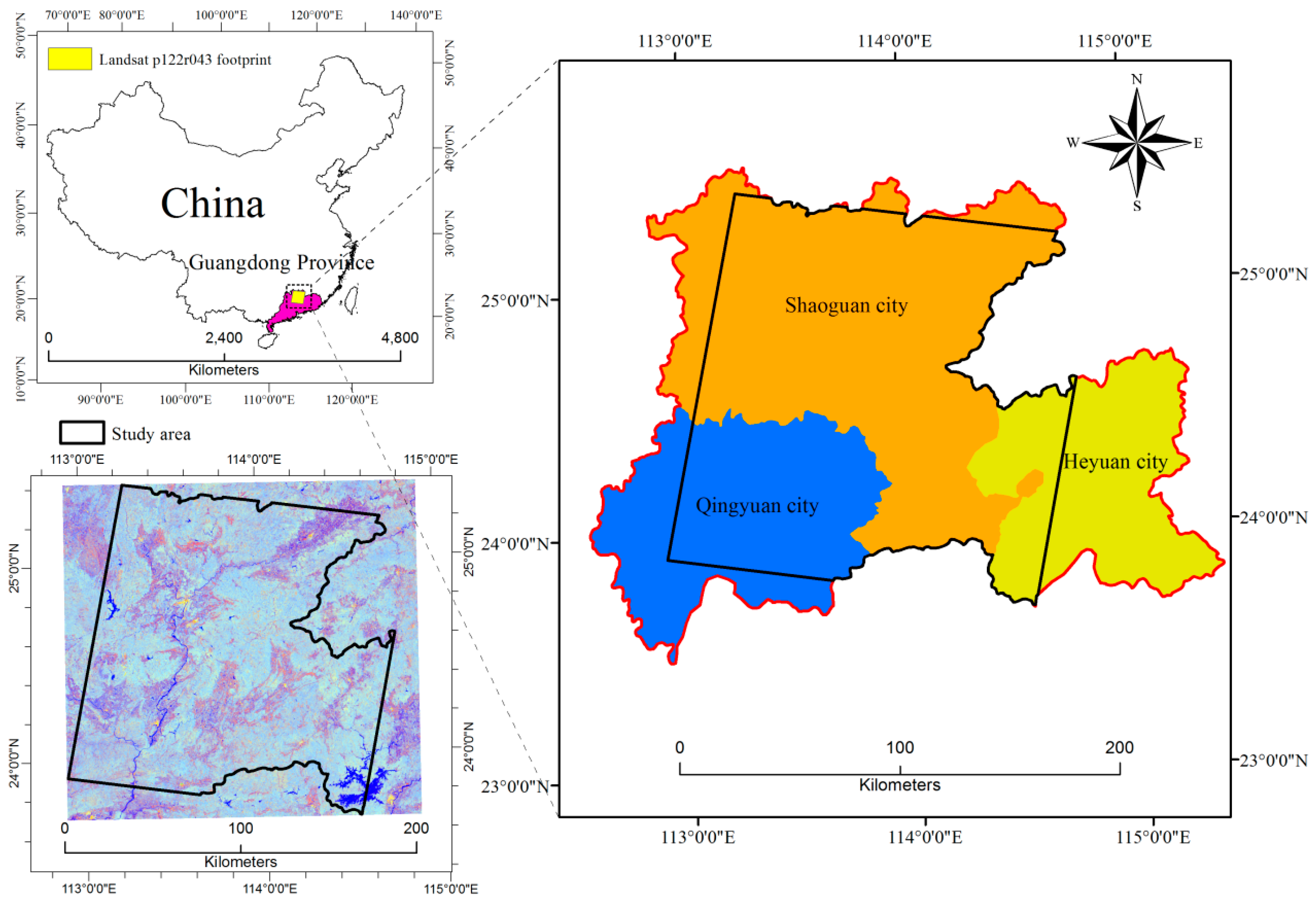
2.1. Study Area
2.2. Data Used and Data Pre-Processing
2.2.1. Field Data
2.2.2. Landsat Data
2.2.3. ALOS PALSAR Data Acquisition and Pre-Processing
2.3. Plot-Level Explanatory Variables
2.4. RF Modeling and Implementation
2.4.1. Variable Selection
2.4.2. Accuracy Assessment and Validation
2.5. Integration of AGB Changes with Forest Disturbance Maps
2.6. Multiple Exploratory Factor Analysis about Potential Factors of Forest AGB Dynamics
3. Results
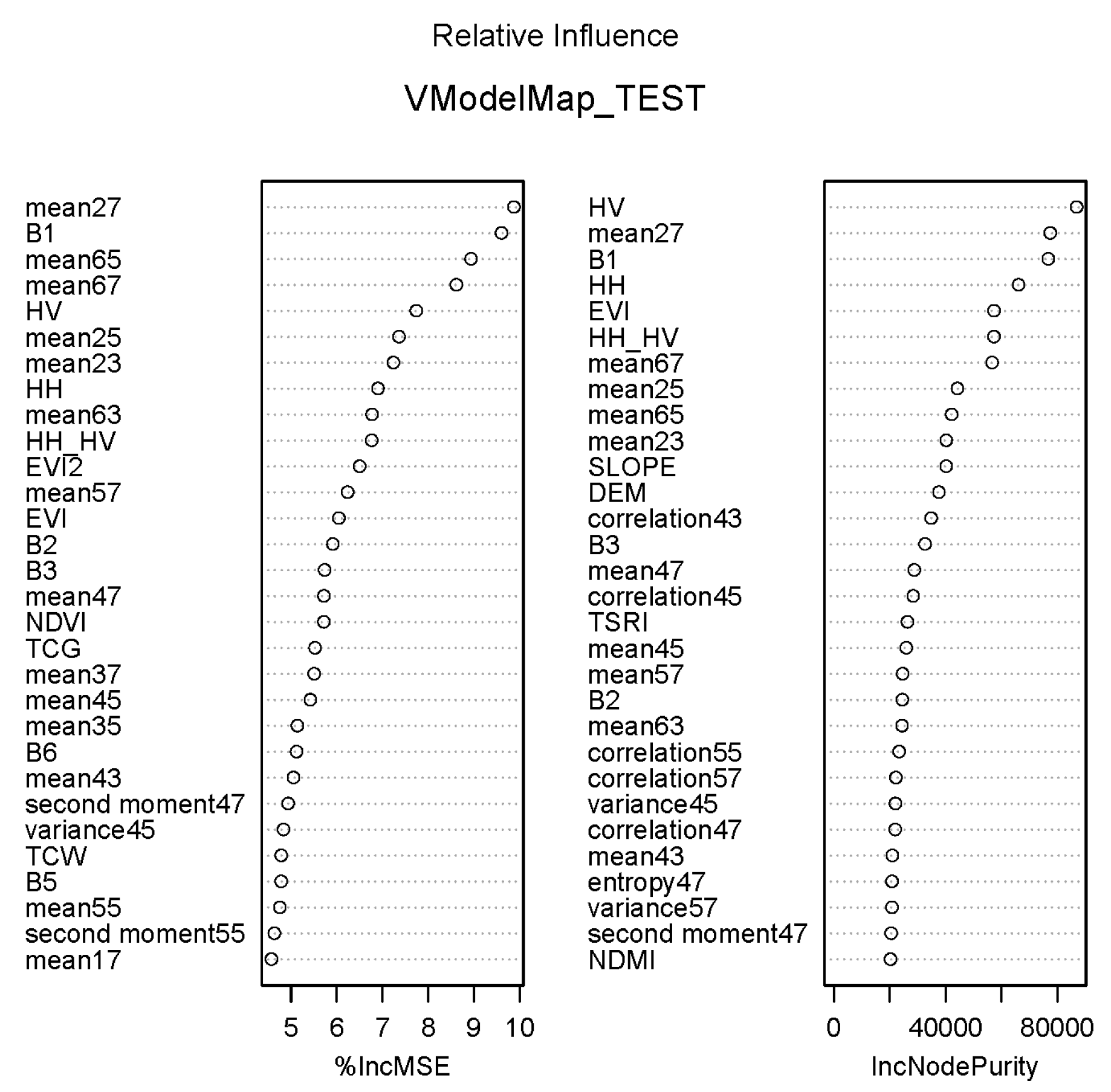
3.1. Variable Importance and Selection
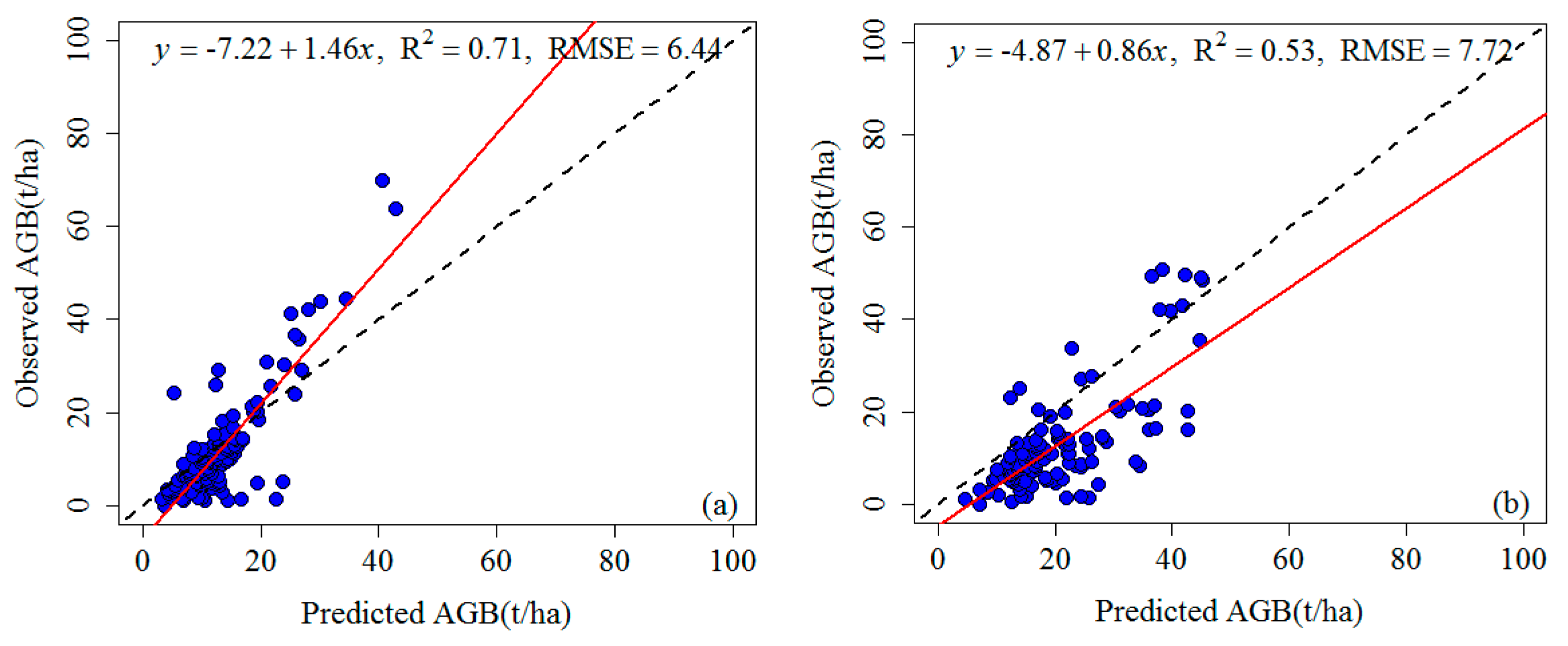
3.2. Predictive Performance of the RF Regression Models
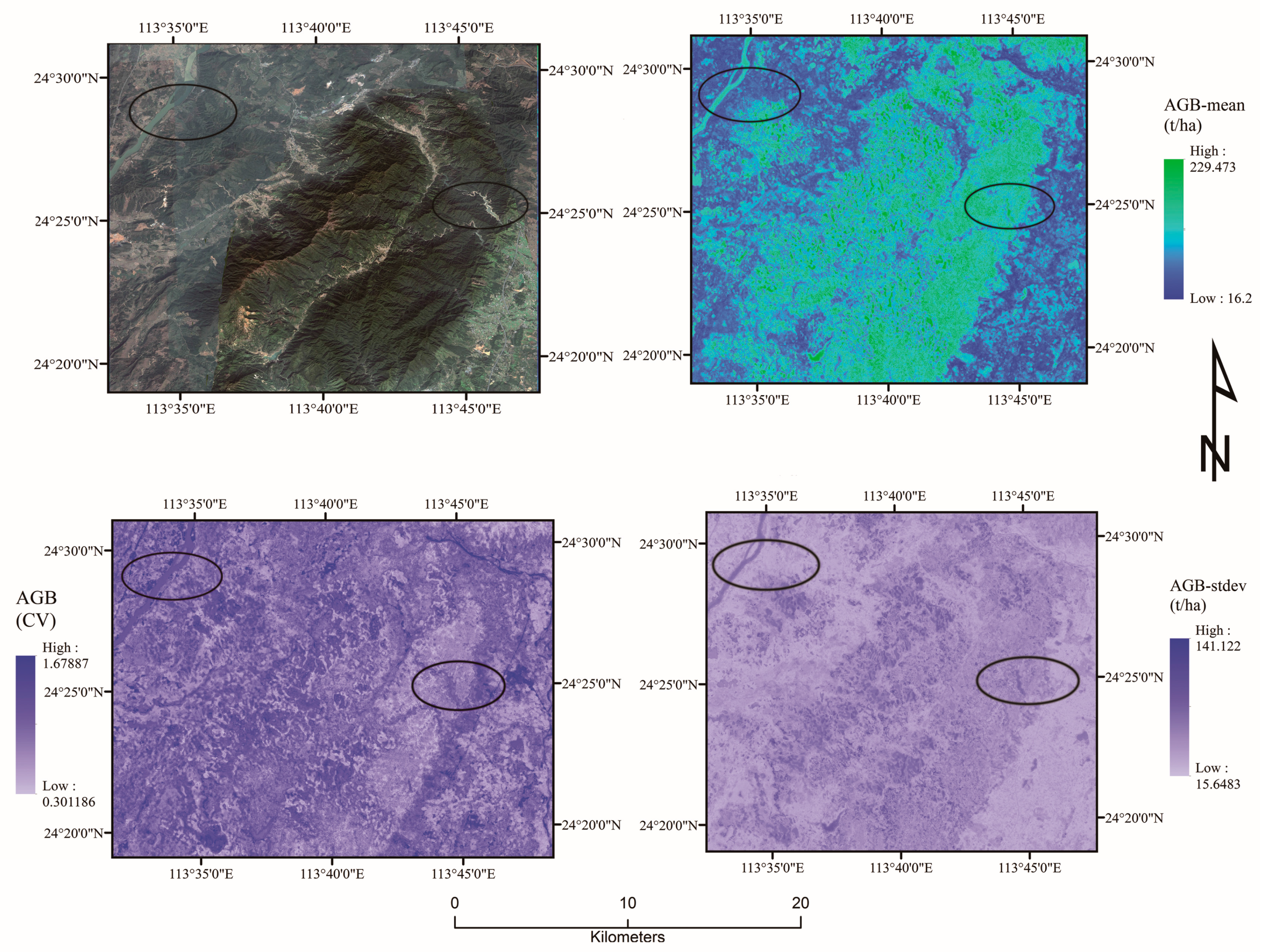
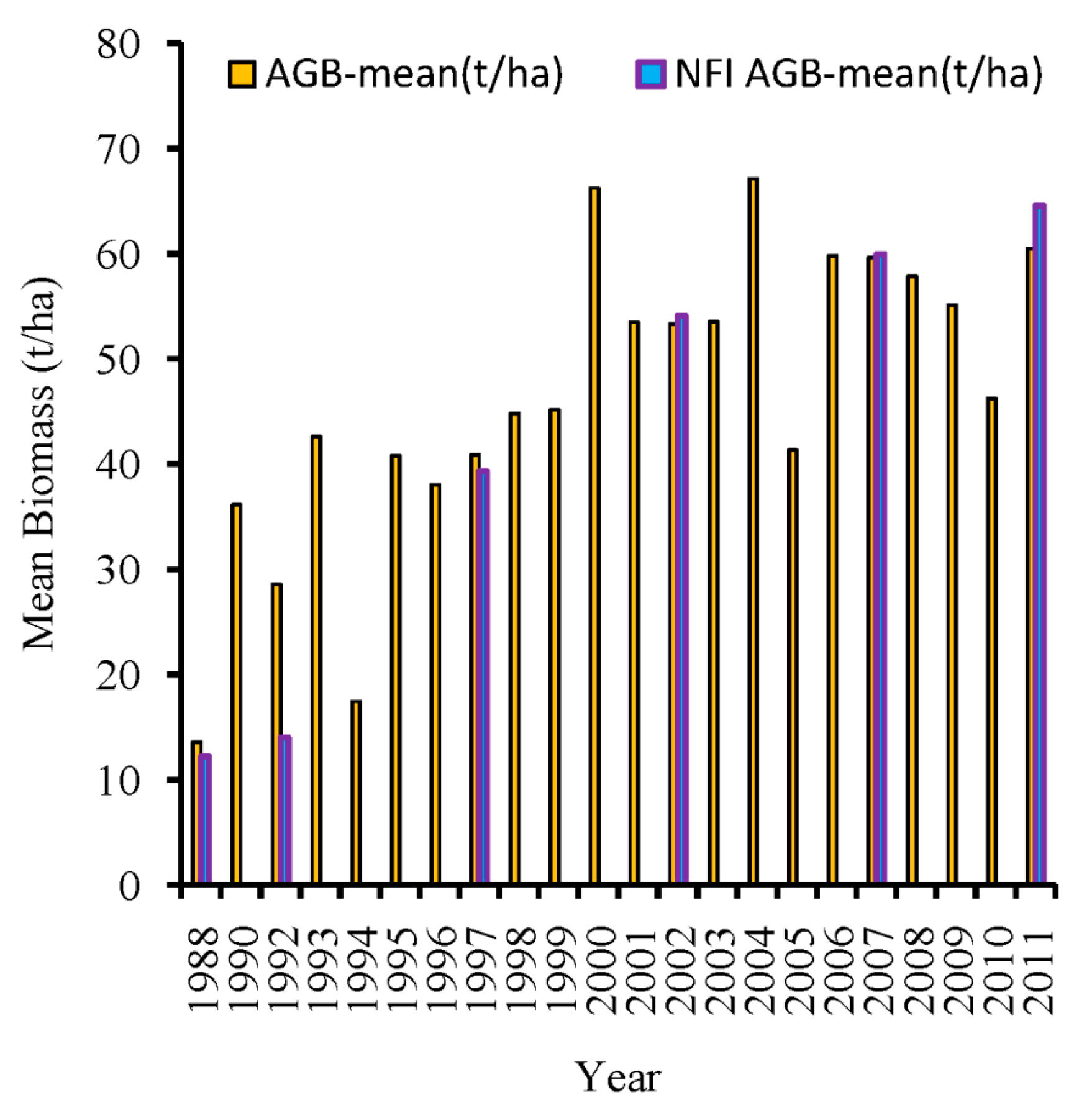
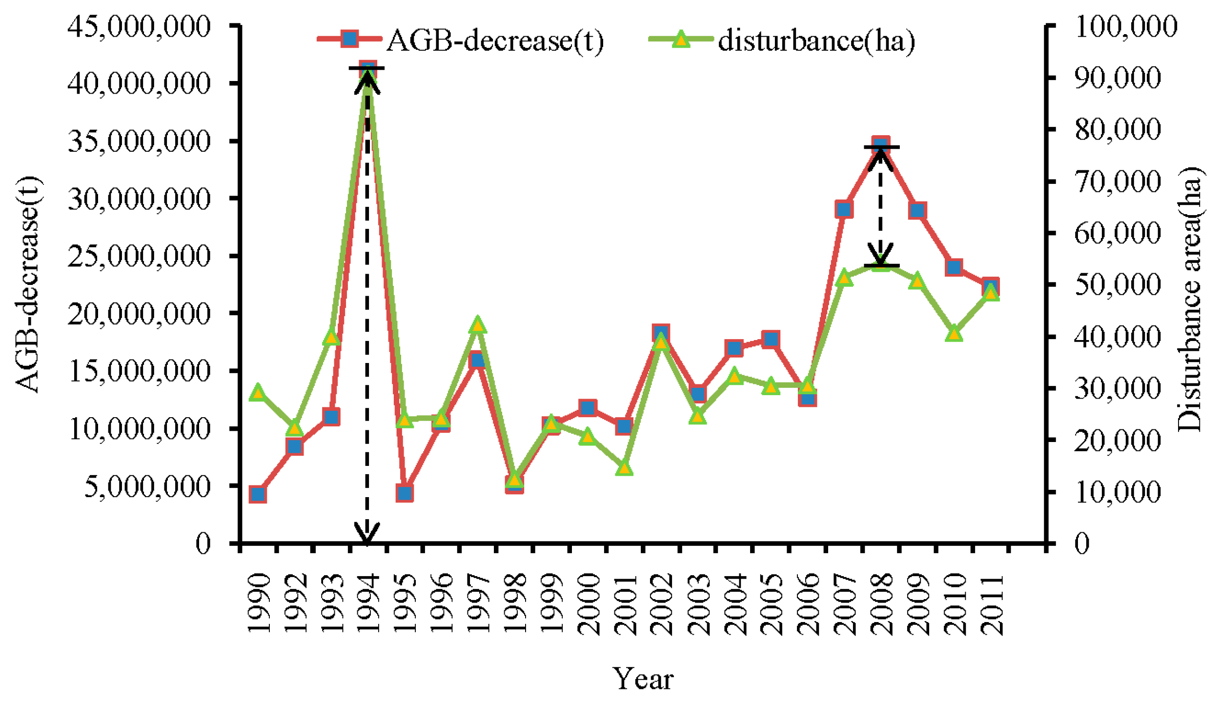
3.3. Forest AGB Dynamics across Northern Guangdong
3.4. Spatio-Temporal Multi-Scale Driving Factors of Forest AGB Dynamics
3.4.1. Regional Climate Change
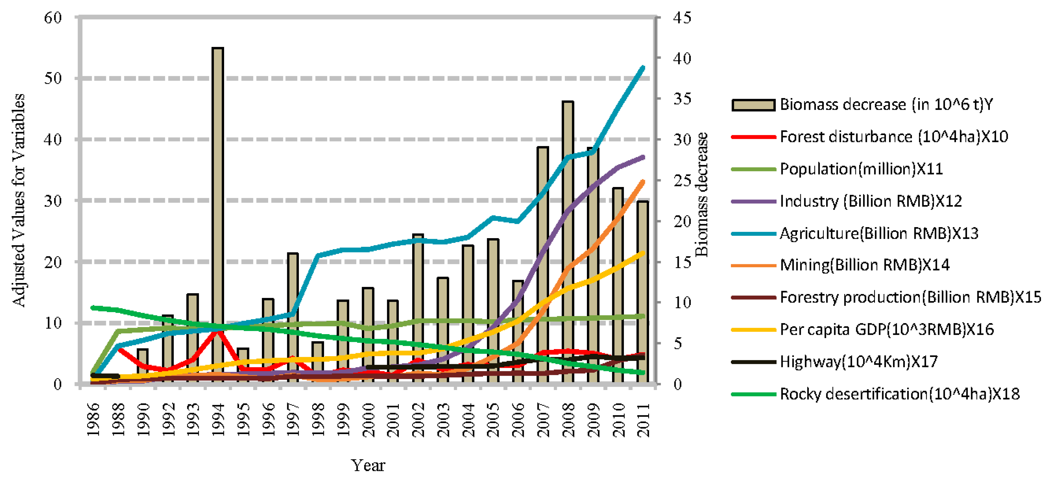
3.4.2. Human Activities
3.4.3. Quantification Analysis of AGB Driving Factors
4. Discussion
4.1. The RF Regression and Predicted Variables Selection
4.1.1. Selection of Field Plot Data and Developing AGB Observations
4.1.2. Image-Based Predicted Variables and Other Ancillary Data
4.1.3. RF Regression and Validation
4.2. Forest AGB and Forest Disturbance Dynamics Change
4.3. Analysis of AGB Drivers
4.3.1. Correlation Analysis
4.3.2. Quantification and Qualitative Analysis
4.4. Uncertainty in Detection of AGB and Forest Disturbance
5. Conclusions
Acknowledgments
Author Contributions
Conflicts of Interest
Appendix

| Tree Species | Equations |
|---|---|
| Cunninghamia Lanceolata | Wt = Ws + Wb + Wl + Wr; |
| Ws = 0.34015 × D−0.39239 × H0.40890 × V; Wb = 0.27140 × D1.07261 × H−1.69157 × V; | |
| Wl = 0.510239 × D0.69072 × H−1.71327 × V; Wr = 0.46493 × D−0.32802 × H−0.28171 × V. | |
| Pinus Elliottii Engelm | Wt = Ws + Wb + Wl + Wr; |
| Ws = 0.20011 × D0.173698 × H0.086849 × V; Wb = 0.019166 × D0.62501 × V; | |
| Wl = 0.57342 × D−0.59891 × V; Wr = 0.46493 × D−0.61082 × V. | |
| Broad-leave trees | Wt = Ws + Wb + Wl + Wr; |
| Ws = 0.29700 × D0.21272 × H0.046734 × V; Wb = 0.54541 × D−0.27401 × H−0.16565 × V; | |
| Wl = 0.22526 × D−0.38874 × H−0.21925 × V; Wr = 0.820322 × D−0.39686 × H−0.22275 × V. | |
| Sundry bamboo | Wt = Ws + Wb + Wl + Wr; |
| Ws = 0.001 × N × e3.27482−9.6724/D; Wb = 0.001 × N/(0.685 + 12.8983 × e−D); | |
| Wl = 0.001 × N/(1.056 + 48.5609 × e−D); Wr = 0.001 × N/(0.462 + 12.8510 × e−D). | |
| Pinus massoniana | Wt = Ws + Wb + Wl + Wr; |
| Ws = 0.29289 × D0.14621 × H0.0089524 × V; Wb = 0.12532 × V; | |
| Wl = 0.079612 × D−0.35263 × H0.015724 × V; Wr = 0.48437 × D−0.62207 × H0.029132 × V. | |
| Eucalyptus | Wt = Ws + Wb + Wl + Wr; |
| Ws = 0.23719 × D0.31557 × H−0.022517 × V; Wb = 0.090123 × D−0.30267 × H0.019109 × V; | |
| Wl = 0.052637 × D−0.21666 × H0.014372 × V; Wr = 0.15553 × D−0.09897 × H0.0073208 × V. | |
| Phyllostachys edulis | Wt = Ws + Wb + Wl + Wr; |
| Ws = 0.0000967 × D2.175 × N; Wb = 0.00083198 × D1.1774 × N0.648; | |
| Wl = 0.0005099 × D1.1774 × N0.648; Wr = 0.000024175 × D2.175 × N +0.000335475 × D1.1774 × N0.648. | |
| Rhodomyrtustomentosa | Wt = 0.844764 × G0.57041 × H0.91788. |
| Miscellaneous shrubs | Wt = 0.056928 × G1.25437 × H0.662068. |
| Baeckeafrutescens | Wt = 0.20784 × G0.78701 × H0.55053. |
| Bamboo shrubs | Wt = 0.0538344 × G1.18518 × H0.33621. |
References
- Houghton, R.A. Aboveground forest biomass and the global carbon balance. Glob. Chang. Biol. 2005, 11, 945–958. [Google Scholar] [CrossRef]
- IPCC. Climate Change 2014: Mitigation of Climate Change; Contribution of Working Group III to the Fifth Assessment Report of the Intergovernmental Panel on Climate Change; Cambridge University Press: Cambridge, UK; New York, NY, USA, 2014. [Google Scholar]
- Schroeder, P.; Brown, S.; Mo, J.M.; Birdsey, R.; Cieszewski, C. Biomass estimation for temperate broadleaf forests of the united states using inventory data. For. Sci. 1997, 43, 424–434. [Google Scholar]
- Blackard, J.A.; Finco, M.V.; Helmer, E.H.; Holden, G.R.; Hoppus, M.L.; Jacobs, D.M.; Lister, A.J.; Moisen, G.G.; Nelson, M.D.; Riemann, R.; et al. Mapping us forest biomass using nationwide forest inventory data and moderate resolution information. Remote Sens. Environ. 2008, 112, 1658–1677. [Google Scholar] [CrossRef]
- Zhu, X.; Liu, D. Improving forest aboveground biomass estimation using seasonal Landsat NDVI time-series. ISPRS J. Photogramm. 2015, 102, 222–231. [Google Scholar] [CrossRef]
- Su, Y.; Guo, Q.; Xue, B.; Hu, T.; Alvarez, O.; Tao, S.; Fang, J. Spatial distribution of forest aboveground biomass in China: Estimation through combination of spaceborne lidar, optical imagery, and forest inventory data. Remote Sens. Environ. 2016, 173, 187–199. [Google Scholar] [CrossRef]
- Wulder, M.A.; White, J.C.; Fournier, R.A.; Luther, J.E.; Magnussen, S. Spatially explicit large area biomass estimation: Three approaches using forest inventory and remotely sensed imagery in a GIS. Sensors 2008, 8, 529–560. [Google Scholar] [CrossRef]
- Zald, H.S.J.; Wulder, M.A.; White, J.C.; Hilker, T.; Hermosilla, T.; Hobart, G.W.; Coops, N.C. Integrating Landsat pixel composites and change metrics with lidar plots to predictively map forest structure and aboveground biomass in Saskatchewan, Canada. Remote Sens. Environ. 2016, 176, 188–201. [Google Scholar] [CrossRef]
- Lei, X.D.; Tang, M.P.; Lu, Y.C.; Hong, L.X.; Tian, D.L. Forest inventory in china: Status and challenges. Int. For. Rev. 2009, 11, 52–63. [Google Scholar] [CrossRef]
- Xie, X.; Wang, Q.; Dai, L.; Su, D.; Wang, X.; Qi, G.; Ye, Y. Application of China’s national forest continuous inventory database. Environ.Manag. 2011, 48, 1095–1106. [Google Scholar] [CrossRef] [PubMed]
- Gómez, C.; White, J.C.; Wulder, M.A.; Alejandro, P. Historical forest biomass dynamics modelled with Landsat spectral trajectories. ISPRS J. Photogramm. 2014, 93, 14–28. [Google Scholar] [CrossRef] [Green Version]
- Hansen, M.C.; Potapov, P.V.; Moore, R.; Hancher, M.; Turubanova, S.A.; Tyukavina, A.; Thau, D.; Stehman, S.V.; Goetz, S.J.; Loveland, T.R.; et al. High-resolution global maps of 21st-century forest cover change. Science 2013, 342, 850–853. [Google Scholar] [CrossRef] [PubMed]
- Lu, D. Aboveground biomass estimation using Landsat TM data in the Brazilian Amazon. Int. J. Remote Sens. 2005, 26, 2509–2525. [Google Scholar] [CrossRef]
- Powell, S.L.; Cohen, W.B.; Healey, S.P.; Kennedy, R.E.; Moisen, G.G.; Pierce, K.B.; Ohmann, J.L. Quantification of live aboveground forest biomass dynamics with Landsat time-series and field inventory data: A comparison of empirical modeling approaches. Remote Sens. Environ. 2010, 114, 1053–1068. [Google Scholar] [CrossRef]
- Roy, D.P.; Wulder, M.A.; Loveland, T.R.; Woodcock, C.E.; Allen, R.G.; Anderson, M.C.; Helder, D.; Irons, J.R.; Johnson, D.M.; Kennedy, R.; et al. Landsat-8: Science and product vision for terrestrial global change research. Remote Sens. Environ. 2014, 145, 154–172. [Google Scholar] [CrossRef]
- Latifi, H.; Fassnacht, F.E.; Hartig, F.; Berger, C.; Hernández, J.; Corvalán, P.; Koch, B. Stratified aboveground forest biomass estimation by remote sensing data. Int. J. Appl. Earth Obs. Geoinf. 2015, 38, 229–241. [Google Scholar] [CrossRef]
- Karlson, M.; Ostwald, M.; Reese, H.; Sanou, J.; Tankoano, B.; Mattsson, E. Mapping tree canopy cover and aboveground biomass in Sudano-Sahelian woodlands using Landsat 8 and random forest. Remote Sens. 2015, 7, 10017–10041. [Google Scholar] [CrossRef]
- Zhang, J.; Huang, S.; Hogg, E.H.; Lieffers, V.; Qin, Y.; He, F. Estimating spatial variation in Alberta forest biomass from a combination of forest inventory and remote sensing data. Biogeosciences 2014, 11, 2793–2808. [Google Scholar] [CrossRef] [Green Version]
- Eckert, S. Improved forest biomass and carbon estimations using texture measures from worldview-2 satellite data. Remote Sens. 2012, 4, 810–829. [Google Scholar] [CrossRef]
- Gwenzi, D.; Lefsky, M.A. Plot-level aboveground woody biomass modeling using canopy height and Auxiliary remote sensing data in a heterogeneous savanna. J. Appl. Remote Sens. 2016, 10. [Google Scholar] [CrossRef]
- Lefsky, M.A.; Harding, D.J.; Keller, M.; Cohen, W.B.; Carabajal, C.C.; Del BomEspirito-Santo, F.; Hunter, M.O.; de Oliveira, R. Estimates of forest canopy height and aboveground biomass using ICESAT. Geophys. Res. Lett. 2005, 32, L22S02. [Google Scholar] [CrossRef]
- Montesano, P.M.; Rosette, J.; Sun, G.; North, P.; Nelson, R.F.; Dubayah, R.O.; Ranson, K.J.; Kharuk, V. The uncertainty of biomass estimates from modeled ICESAT-2 returns across a boreal forest gradient. Remote Sens. Environ. 2015, 158, 95–109. [Google Scholar] [CrossRef]
- Van Leeuwen, M.; Nieuwenhuis, M. Retrieval of forest structural parameters using lidar remote sensing. Eur. J. For. Res. 2010, 129, 749–770. [Google Scholar] [CrossRef]
- Zhang, G.; Ganguly, S.; Nemani, R.R.; White, M.A.; Milesi, C.; Hashimoto, H.; Wang, W.; Saatchi, S.; Yu, Y.; Myneni, R.B. Estimation of forest aboveground biomass in California using canopy height and leaf area index estimated from satellite data. Remote Sens. Environ. 2014, 151, 44–56. [Google Scholar] [CrossRef]
- Main-Knorn, M.; Cohen, W.B.; Kennedy, R.E.; Grodzki, W.; Pflugmacher, D.; Griffiths, P.; Hostert, P. Monitoring coniferous forest biomass change using a Landsat trajectory-based approach. Remote Sens. Environ. 2013, 139, 277–290. [Google Scholar] [CrossRef]
- Avitabile, V.; Baccini, A.; Friedl, M.A.; Schmullius, C. Capabilities and limitations of Landsat and land cover data for aboveground woody biomass estimation of Uganda. Remote Sens. Environ. 2012, 117, 366–380. [Google Scholar] [CrossRef]
- Du, L.; Zhou, T.; Zou, Z.; Zhao, X.; Huang, K.; Wu, H. Mapping forest biomass using remote sensing and national forest inventory in china. Forests 2014, 5, 1267–1283. [Google Scholar] [CrossRef]
- Dube, T.; Mutanga, O. Evaluating the utility of the medium-spatial resolution Landsat 8 multispectral sensor in quantifying aboveground biomass in Umgeni catchment, South Africa. ISPRS J. Photogramm. 2015, 101, 36–46. [Google Scholar] [CrossRef]
- Dube, T.; Mutanga, O. Investigating the robustness of the new Landsat-8 operational land imager derived texture metrics in estimating plantation forest aboveground biomass in resource constrained areas. ISPRS J. Photogramm. 2015, 108, 12–32. [Google Scholar] [CrossRef]
- Dube, T.; Mutanga, O.; Adam, E.; Ismail, R. Intra-and-inter species biomass prediction in a plantation forest: Testing the utility of high spatial resolution spaceborne multispectral RapidEye sensor and advanced machine learning algorithms. Sensors 2014, 14, 15348–15370. [Google Scholar] [CrossRef] [PubMed]
- Main-Knorn, M.; Moisen, G.G.; Healey, S.P.; Keeton, W.S.; Freeman, E.A.; Hostert, P. Evaluating the remote sensing and inventory-based estimation of biomass in the western Carpathians. Remote Sens. 2011, 3, 1427–1446. [Google Scholar] [CrossRef]
- Cartus, O.; Santoro, M.; Kellndorfer, J. Mapping forest aboveground biomass in the Northeastern United States with ALOS PALSAR dual-polarization L-band. Remote Sens. Environ. 2012, 124, 466–478. [Google Scholar] [CrossRef]
- Da Silva Ramos Vieira Martins, F.; dos Santos, J.R.; Galvão, L.S.; Xaud, H.A.M. Sensitivity of ALOS/PALSAR imagery to forest degradation by fire in Northern Amazon. Int. J. Appl. Earth Obs. Geoinf. 2016, 49, 163–174. [Google Scholar] [CrossRef]
- Mermoz, S.; Le Toan, T. Forest disturbances and regrowth assessment using ALOS PALSAR data from 2007 to 2010 in Vietnam, Cambodia and Lao PDR. Remote Sens. 2016, 8, 217. [Google Scholar] [CrossRef]
- Peregon, A.; Yamagata, Y. The use of ALOS/PALSAR backscatter to estimate above-ground forest biomass: A case study in western Siberia. Remote Sens. Environ. 2013, 137, 139–146. [Google Scholar] [CrossRef]
- Ram Avtar, R.S.; Takeuchi, W.; Sawada, H. PALSAR 50 m mosaic data based national level biomass estimation in Cambodia for implementation of REDD+ mechanism. PLoS ONE 2013. [Google Scholar] [CrossRef]
- Saatchi, S.S.; Moghaddam, M. Estimation of crown and stem water content and biomass of boreal forest using polarimetric SAR imagery. IEEE Trans. Geosci. Remote Sens. 2000, 38, 697–709. [Google Scholar] [CrossRef]
- Lu, D.S. The potential and challenge of remote sensing-based biomass estimation. Int. J. Remote Sens. 2006, 27, 1297–1328. [Google Scholar] [CrossRef]
- Le Toan, T.; Quegan, S.; Woodward, I.; Lomas, M.; Delbart, N.; Picard, G. Relating radar remote sensing of biomass to modelling of forest carbon budgets. Clim. Chang. 2004, 67, 379–402. [Google Scholar] [CrossRef]
- Hansen, M.C.; Loveland, T.R. A review of large area monitoring of land cover change using Landsat data. Remote Sens. Environ. 2012, 122, 66–74. [Google Scholar] [CrossRef]
- Roy, D.P.; Ju, J.C.; Kline, K.; Scaramuzza, P.L.; Kovalskyy, V.; Hansen, M.; Loveland, T.R.; Vermote, E.; Zhang, C.S. Web-enabled Landsat data (weld): Landsat ETM+ composited mosaics of the conterminous United States. Remote Sens. Environ. 2010, 114, 35–49. [Google Scholar] [CrossRef]
- Seidl, R.; Schelhaas, M.J.; Rammer, W.; Verkerk, P.J. Increasing forest disturbances in Europe and their impact on carbon storage. Nat. Clim. Chang. 2014, 4, 806–810. [Google Scholar] [PubMed]
- Zhang, Y.; Liang, S. Changes in forest biomass and linkage to climate and forest disturbances over northeastern china. Glob. Chang. Biol. 2014, 20, 2596–2606. [Google Scholar] [CrossRef] [PubMed]
- Cohen, W.B.; Yang, Z.; Stehman, S.V.; Schroeder, T.A.; Bell, D.M.; Masek, J.G.; Huang, C.; Meigs, G.W. Forest disturbance across the conterminous united states from 1985–2012: The emerging dominance of forest decline. For. Ecol. Manag. 2016, 360, 242–252. [Google Scholar] [CrossRef]
- Huang, C.Q.; Coward, S.N.; Masek, J.G.; Thomas, N.; Zhu, Z.L.; Vogelmann, J.E. An automated approach for reconstructing recent forest disturbance history using dense Landsat time series stacks. Remote Sens. Environ. 2010, 114, 183–198. [Google Scholar] [CrossRef]
- Kennedy, R.E.; Yang, Z.; Cohen, W.B. Detecting trends in forest disturbance and recovery using yearly Landsat time series: 1. LandTrendr—Temporal segmentation algorithms. Remote Sens. Environ. 2010, 114, 2897–2910. [Google Scholar] [CrossRef]
- Masek, J.G.; Huang, C.Q.; Wolfe, R.; Cohen, W.; Hall, F.; Kutler, J.; Nelson, P. North American forest disturbance mapped from a decadal Landsat record. Remote Sens. Environ. 2008, 112, 2914–2926. [Google Scholar] [CrossRef]
- Pflugmacher, D.; Cohen, W.B.; Kennedy, R.E.; Yang, Z. Using Landsat-derived disturbance and recovery history and lidar to map forest biomass dynamics. Remote Sens. Environ. 2014, 151, 124–137. [Google Scholar] [CrossRef]
- Powell, S.L.; Cohen, W.B.; Kennedy, R.E.; Healey, S.P.; Huang, C. Observation of trends in biomass loss as a result of disturbance in the conterminous U.S.: 1986–2004. Ecosystems 2013, 17, 142–157. [Google Scholar] [CrossRef]
- Masek, J.G.; Vermote, E.F.; Saleous, N.E.; Wolfe, R.; Hall, F.G.; Huemmrich, K.F.; Gao, F.; Kutler, J.; Lim, T.K. A Landsat surface reflectance dataset for North America, 1990–2000. IEEE Geosci. Remote Sens. Lett. 2006, 3, 68–72. [Google Scholar] [CrossRef]
- Canty, M.J.; Nielsen, A.A. Automatic radiometric normalization of multitemporal satellite imagery with the iteratively re-weighted mad transformation. Remote Sens. Environ. 2008, 112, 1025–1036. [Google Scholar] [CrossRef]
- Hamdan, O.; Khali Aziz, H.; MohdHasmadi, I. L-band ALOSPALSAR for biomass estimation of Matang mangroves, Malaysia. Remote Sens. Environ. 2014, 155, 69–78. [Google Scholar] [CrossRef]
- Shimada, M.; Isoguchi, O.; Tadono, T.; Isono, K. PALSAR radiometric and geometric calibration. IEEE Trans. Geosci. Remote Sens. 2009, 47, 3915–3932. [Google Scholar] [CrossRef]
- Lee, J.S.; Wen, J.H.; Ainsworth, T.L.; Chen, K.S.; Chen, A.J. Improved sigma filter for speckle filtering of SAR imagery. IEEE Trans. Geosci. Remote Sens. 2009, 47, 202–213. [Google Scholar]
- Rouse, J.W.; Haas, R.H.; Schell, J.A.; Deering, D.W. Monitoring vegetation systems in the Great Plains with erst. NASA Spec. Publ. 1973, 351, 309–317. [Google Scholar]
- Gao, B.C. NDWI—A normalized difference water index for remote sensing of vegetation liquid water from space. Remote Sens. Environ. 1996, 58, 257–266. [Google Scholar] [CrossRef]
- McFeeters, S.K. The use of the normalized difference water index (NDWI) in the delineation of open water features. Int. J. Remote Sens. 1996, 17, 1425–1432. [Google Scholar] [CrossRef]
- Xu, H.Q. Modification of normalized difference water index (NDWI) to enhance open water features in remotely sensed imagery. Int. J. Remote Sens. 2006, 27, 3025–3033. [Google Scholar] [CrossRef]
- Miura, T.; Yoshioka, H.; Fujiwara, K.; Yamamoto, H. Inter-comparison of aster and MODIS surface reflectance and vegetation index products for synergistic applications to natural resource monitoring. Sensors 2008, 8, 2480–2499. [Google Scholar] [CrossRef]
- Hunt, E.R.; Daughtry, C.S.T.; Eitel, J.U.H.; Long, D.S. Remote sensing leaf chlorophyll content using a visible band index. Agron. J. 2011, 103, 1090–1099. [Google Scholar] [CrossRef]
- Huete, A.; Didan, K.; Miura, T.; Rodriguez, E.P.; Gao, X.; Ferreira, L.G. Overview of the radiometric and biophysical performance of the MODIS vegetation indices. Remote Sens. Environ. 2002, 83, 195–213. [Google Scholar] [CrossRef]
- Wu, W.C. The generalized difference vegetation index (GDVI) for dryland characterization. Remote Sens. 2014, 6, 1211–1233. [Google Scholar] [CrossRef]
- Lymburner, L.; Beggs, P.J.; Jacobson, C.R. Estimation of canopy-average surface-specific leaf area using Landsat TM data. Photogramm. Eng. Remote Sens. 2000, 66, 183–191. [Google Scholar]
- Birth, G.S.; McVey, G.R. Measuring the color of growing turf with a reflectance spectrophotometer. Agron. J. 1968, 60, 640–643. [Google Scholar] [CrossRef]
- Crist, E.P.; Cicone, R.C. A physically-based transformation of thematic mapper data—The TM tasseled cap. IEEE Trans. Geosci. Remote Sens. 1984, 22, 256–263. [Google Scholar] [CrossRef]
- Duane, M.V.; Cohen, W.B.; Campbell, J.L.; Hudiburg, T.; Turner, D.P.; Weyermann, D.L. Implications of alternative field-sampling designs on Landsat-based mapping of stand age and carbon stocks in Oregon forests. For. Sci. 2010, 56, 405–416. [Google Scholar]
- Roberts, D.W.; Cooper, S.V. Concepts and techniques of vegetation mapping. Land Classifications based on vegetation: Applications for resource management; Ferguson, D., Morgan, P., Johnson, F.D., Eds.; USDA Forest Service General Technical Report INT-257; USDA: Ogden, Utah; pp. 90–96.
- Haralick, R.M.; Shanmuga, K.; Dinstein, I. Textural features for image classification. IEEE Trans. Syst. Man Cybern. 1973, 3, 610–621. [Google Scholar] [CrossRef]
- Breiman, L. Random forests. Mach. Learn. 2001, 45, 5–32. [Google Scholar] [CrossRef]
- Freeman, E.A.; Moisen, G.G.; Coulston, J.W.; Wilson, B.T. Random forests and stochastic gradient boosting for predicting tree canopy cover: Comparing tuning processes and model performance1. Can. J. For. Res. 2016, 46, 323–339. [Google Scholar] [CrossRef]
- Freeman, E.A.; Frescino, T.S.; Moisen, G.G. ModelMap: An R Package for Model Creation and Map Production. Available online: https://cran.r-project.org/web/packages/ModelMap/ModelMap.pdf (accessed on 2 July 2016).
- Liaw, A.; Matthew, W. Classification and regression by randomforest. R News 2002, 2, 18–22. [Google Scholar]
- Thomas, N.E.; Huang, C.Q.; Goward, S.N.; Powell, S.; Schleeweis, K.; Hinds, A. Validation of North American forest disturbance dynamics derived from Landsat time series stacks. Remote Sens. Environ. 2011, 115, 19–32. [Google Scholar] [CrossRef]
- Schroeder, T.A.; Healey, S.P.; Moisen, G.G.; Frescino, T.S.; Cohen, W.B.; Huang, C.; Kennedy, R.E.; Yang, Z. Improving estimates of forest disturbance by combining observations from Landsat time series with U.S. Forest service forest inventory and analysis data. Remote Sens. Environ. 2014, 154, 61–73. [Google Scholar] [CrossRef]
- Li, S.; Wei, X.H.; Huang, J.G.; Wang, X.Z.; Lu, G.Y.; Li, H.X. The causes and processes responsible for rocky desertification in karst areas of southern China. Sci. Cold Arid Reg. 2009, 1, 80–90. [Google Scholar]
- Kaiser, H.F. The varimax criterion for analytic rotation in factor-analysis. Psychometrika 1958, 23, 187–200. [Google Scholar] [CrossRef]
- Kelsey, K.; Neff, J. Estimates of aboveground biomass from texture analysis of Landsat imagery. Remote Sens. 2014, 6, 6407–6422. [Google Scholar] [CrossRef]
- Champion, I.; Dubois-Fernandez, P.; Guyon, D.; Cottrel, M. Radar image texture as a function of forest stand age. Int. J. Remote Sens. 2008, 29, 1795–1800. [Google Scholar] [CrossRef]
- Mermoz, S.; Toan, T.L.; Villard, L.; Rejou-Mechain, M.; Seifert-Granzin, J. Biomass assessment in the Cameroon savanna using ALOS PALSAR data. Remote Sens. Environ. 2014, 155, 109–119. [Google Scholar] [CrossRef]
- Carreiras, J.M.B.; Vasconcelos, M.J.; Lucas, R.M. Understanding the relationship between aboveground biomass and ALOS PALSAR data in the forests of Guinea-Bissau (West Africa). Remote Sens. Environ. 2012, 121, 426–442. [Google Scholar] [CrossRef]
- Gunlu, A.; Ercanli, I.; Baskent, E.Z.; Cakir, G. Estimating aboveground biomass using Landsat TM imagery: A case study of Anatolian Crimean pine forests in turkey. Ann. For. Res. 2014, 57, 289–298. [Google Scholar]
- Xiao, X.M.; Hollinger, D.; Aber, J.; Goltz, M.; Davidson, E.A.; Zhang, Q.Y.; Moore, B. Satellite-based modeling of gross primary production in an evergreen needle leaf forest. Remote Sens. Environ. 2004, 89, 519–534. [Google Scholar] [CrossRef]
- Hantson, S.; Chuvieco, E. Evaluation of different topographic correction methods for Landsat imagery. Int. J. Appl. Earth Obs. Geoinf. 2011, 13, 691–700. [Google Scholar] [CrossRef]
- Zhang, J.Y.; Dai, M.H.; Wang, L.C.; Zeng, C.F.; Su, W.C. The challenge and future of rocky desertification control in karst areas in southwest China. Solid Earth 2016, 7, 83–91. [Google Scholar] [CrossRef]
- Jiang, Z.; Lian, Y.; Qin, X. Rocky desertification in southwest china: Impacts, causes, and restoration. Earth Sci. Rev. 2014, 132, 1–12. [Google Scholar] [CrossRef]
- Stone, R. Natural disasters—Ecologists report huge storm losses in China’s forests. Science 2008, 319, 1318–1319. [Google Scholar] [CrossRef] [PubMed]
- Stegen, J.C.; Swenson, N.G.; Enquist, B.J.; White, E.P.; Phillips, O.L.; Jorgensen, P.M.; Weiser, M.D.; Mendoza, A.M.; Vargas, P.N. Variation in above-ground forest biomass across broad climatic gradients. Glob. Ecol. Biogeogr. 2011, 20, 744–754. [Google Scholar] [CrossRef]
- Li, X.; Ye, D.; Liang, H.; Zhu, H.; Qin, L.; Zhu, Y.; Wen, Y. Effects of successive rotation regimes on carbon stocks in eucalyptus plantations in subtropical China measured over a full rotation. PLoS ONE 2015, 10, e0132858. [Google Scholar] [CrossRef] [PubMed]
- Wen, Y.G.; Ye, D.; Chen, F.; Liu, S.R.; Liang, H.W. The changes of understory plant diversity in continuous cropping system of eucalyptus plantations, south China. J. For. Res. Jpn. 2010, 15, 252–258. [Google Scholar] [CrossRef]
- Sun, Y.X.; Wu, J.P.; Shao, Y.H.; Zhou, L.X.; Mai, B.X.; Lin, Y.B.; Fu, S.L. Responses of soil microbial communities to prescribed burning in two paired vegetation sites in southern China. Ecol. Res. 2011, 26, 669–677. [Google Scholar] [CrossRef]
- Dale, V.H.; Joyce, L.A.; McNulty, S.; Neilson, R.P.; Ayres, M.P.; Flannigan, M.D.; Hanson, P.J.; Irland, L.C.; Lugo, A.E.; Peterson, C.J.; et al. Climate change and forest disturbances. Bioscience 2001, 51, 723–734. [Google Scholar] [CrossRef]
- Shendryk, I.; Hellstrom, M.; Klemedtsson, L.; Kljun, N. Low-density lidar and optical imagery for biomass estimation over boreal forest in Sweden. Forests 2014, 5, 992–1010. [Google Scholar] [CrossRef]


| Year | Plots (No.) | Min AGB (t/ha) | Max AGB (t/ha) | Mean AGB (t/ha) | Std. Dev. AGB (t/ha) |
|---|---|---|---|---|---|
| 1988 | 165 | 0.06 | 70.06 | 12.25 | 11.89 |
| 1992 | 194 | 0.04 | 52.18 | 14.04 | 13.33 |
| 1997 | 228 | 0.89 | 213.38 | 39.32 | 37.35 |
| 2002 | 253 | 1.99 | 256.31 | 54.08 | 45.24 |
| 2007 | 269 | 2.11 | 323.14 | 59.92 | 51.04 |
| 2012 | 246 | 0.11 | 391.91 | 64.56 | 53.33 |
| Data Source | Sensor | Year/DOY |
|---|---|---|
| USGS | L5 TM | 1990206, 1993278, 1995284, 1996159, 1996191, 2001252, 2003290, 2004277, 2005199, 2006266, 2007205, 2008208, 2009290, 2010213, 2011232 |
| L7 ETM+ | 1999255, 1999287, 2000258, 2001260, 2002311 | |
| BJGS-China | L5 TM | 1986307, 1988313, 1992212, 1994313, 1997305, 1998228 |
| Japan | ALOS PALSAR | 2007, 2008, 2009, 2010 (mosaic) |
| Type | Variable | Formula | Ref. | Description |
|---|---|---|---|---|
| Spectral indices | R, G, B, NIR, SWIR1, SWIR2 | Landsat 5, 7 bands | ||
| NDVI | (NIR − R)/(NIR + R) | [55] | Normalized Difference Vegetation Index | |
| NDMI | (NIR − SWIR)/(NIR + SWIR) | [56] | Normalized Difference Moisture Index | |
| NDWI | (G − NIR)/(G + NIR) | [57] | Normalized Difference Water Index | |
| MNDWI | (G − SWIR)/(G + SWIR) | [58] | Modified Normalized Difference Water Index | |
| EVI2 | 2.5×(NIR − R)/(NIR + 2.4 × R + 1) | [59] | Enhanced vegetation index 2 | |
| CVI | NIR × R/G2 | [60] | chlorophyll vegetation index | |
| EVI | 2.5×(NIR − R)/(NIR + 6 × R − 7.5 × B + 1) | [61] | Enhanced vegetation index | |
| GDVI | (NIR2 − R2)/(NIR2 + R2) | [62] | Generalized Difference Vegetation Index | |
| SLAVI | NIR/(R + SWIR) | [63] | Specific Leaf Area Vegetation Index | |
| SR | NIR/R | [64] | Simple Ratio (SR) | |
| Tasseled cap transformations | TCB, TCG, TCW | [65] | Brightness, Greenness, Wetness | |
| TCA | arctan(TCG/TCB) | [14] | Tasseled cap angle | |
| TCD | [66] | Tasseled cap distance | ||
| Topography | Elevation, SLOPE | |||
| TSRI | 1 − cos((pi/180)(aspect − 30))/2 | [67] | Topographic solar radiation index | |
| Texture(window sizes 3 × 3, 5 × 5, 7 × 7 pixels) | mean, variance, homogeneity, contrast, dissimilarity, entropy, second moment, correlation | [68] | GLCM texture measures | |
| PALSAR | HH, HV, HH/HV | PALSAR components |
| Year | 1988 | 1992 | 1997 | 2002 | 2006 | 2011 |
|---|---|---|---|---|---|---|
| No. of pixels | 117 | 128 | 153 | 172 | 177 | 162 |
| Observed AGB (t/ha) | 0.06–70.06 | 0.04–50.7 | 0.90–213 | 2.40–256 | 2.60–323.1 | 0.89–391.91 |
| Observed-Mean (t/ha) | 12.39 | 12.92 | 40.27 | 59.82 | 63.84 | 67.19 |
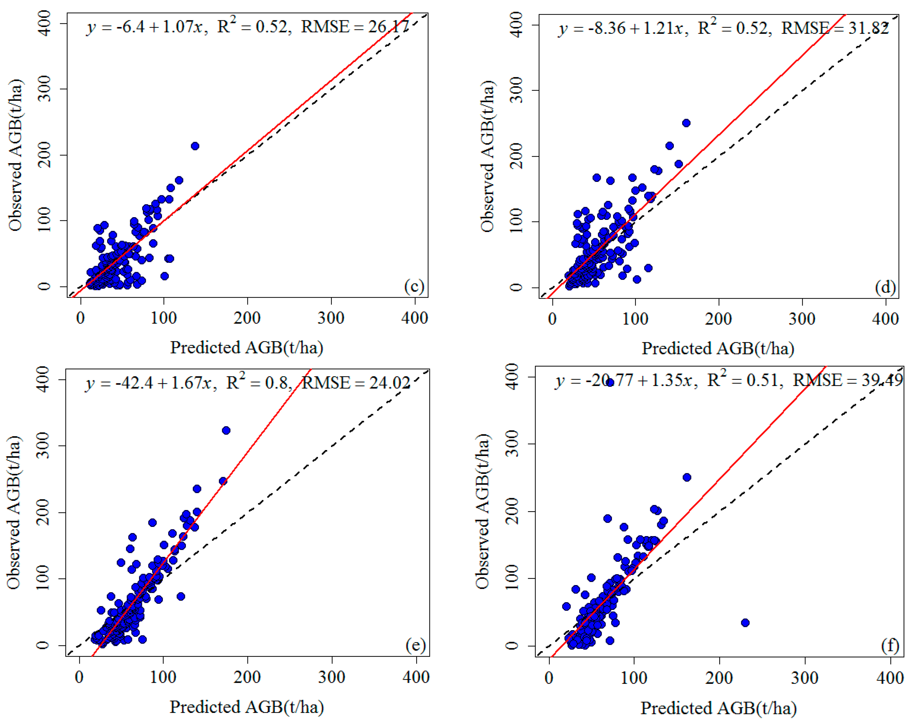
| Predicted AGB (t/ha) | 3.20–42.82 | 4.60–48 | 10–136.80 | 19–161 | 18–175 | 20–229.50 |
| Predicted-Mean (t/ha) | 13.47 | 22.00 | 43.77 | 56.04 | 63.64 | 65.38 |
| R2 | 0.71 | 0.53 | 0.52 | 0.52 | 0.80 | 0.51 |
| RMSE (t/ha) | 6.44 | 7.72 | 26.17 | 31.82 | 24.02 | 39.49 |
| MAE (t/ha) | 5.06 | 9.32 | 19.50 | 23.84 | 22.39 | 24.4 |
| NRMSE (%) | 9.20 | 15.22 | 12.32 | 12.83 | 7.49 | 10.10 |
| X1 | X2 | X3 | X4 | X5 | X6 | X7 | X8 | X9 | |
|---|---|---|---|---|---|---|---|---|---|
| Y | −0.16 | 0.08 | −0.17 | −0.05 | −0.18 | 0.14 | −0.24 | −0.26 | 0.06 |
| X10 | X11 | X12 | X13 | X14 | X15 | X16 | X17 | X18 | |
|---|---|---|---|---|---|---|---|---|---|
| Y | 0.86 | 0.63 | 0.68 | 0.67 | 0.85 | 0.64 | 0.65 | 0.76 | 0.60 |
| Loading Matrix | F1 | F2 | F3 | Loading Matrix | F1 | F2 | F3 |
|---|---|---|---|---|---|---|---|
| X1(mean temperature) | −0.206 | 0.943 | −0.193 | X10 (forest disturbance) | 0.156 | −0.716 | −0.286 |
| X2 (mean maximum temperature) | 0.065 | 0.830 | −0.493 | X11 (population) | 0.936 | 0.039 | −0.151 |
| X3(mean minimum temperature) | −0.318 | 0.861 | 0.161 | X12 (industrial production) | 0.859 | −0.492 | 0.027 |
| X4(annual precipitation) | −0.077 | 0.083 | 0.931 | X13 (agricultural production) | 0.934 | −0.274 | 0.068 |
| X5(extreme low temperature) | −0.864 | 0.039 | −0.183 | X14 (mining) | 0.806 | −0.574 | 0.027 |
| X6(extreme high temperature) | −0.341 | 0.177 | −0.504 | X15 (forestry production) | 0.769 | −0.478 | 0.094 |
| X7 (mean humidity) | −0.293 | 0.266 | 0.537 | X16 (per capita GDP) | 0.909 | −0.409 | 0.018 |
| X8 (min humidity) | −0.693 | 0.362 | −0.115 | X17 (highway mileage) | 0.967 | −0.061 | 0.012 |
| X9 (maximum daily precipitation) | 0.262 | −0.144 | 0.605 | X18 (rock desertification area) | −0.989 | 0.006 | −0.011 |
© 2016 by the authors; licensee MDPI, Basel, Switzerland. This article is an open access article distributed under the terms and conditions of the Creative Commons Attribution (CC-BY) license (http://creativecommons.org/licenses/by/4.0/).
Share and Cite
Shen, W.; Li, M.; Huang, C.; Wei, A. Quantifying Live Aboveground Biomass and Forest Disturbance of Mountainous Natural and Plantation Forests in Northern Guangdong, China, Based on Multi-Temporal Landsat, PALSAR and Field Plot Data. Remote Sens. 2016, 8, 595. https://doi.org/10.3390/rs8070595
Shen W, Li M, Huang C, Wei A. Quantifying Live Aboveground Biomass and Forest Disturbance of Mountainous Natural and Plantation Forests in Northern Guangdong, China, Based on Multi-Temporal Landsat, PALSAR and Field Plot Data. Remote Sensing. 2016; 8(7):595. https://doi.org/10.3390/rs8070595
Chicago/Turabian StyleShen, Wenjuan, Mingshi Li, Chengquan Huang, and Anshi Wei. 2016. "Quantifying Live Aboveground Biomass and Forest Disturbance of Mountainous Natural and Plantation Forests in Northern Guangdong, China, Based on Multi-Temporal Landsat, PALSAR and Field Plot Data" Remote Sensing 8, no. 7: 595. https://doi.org/10.3390/rs8070595