An Operational Framework for Land Cover Classification in the Context of REDD+ Mechanisms. A Case Study from Costa Rica

Abstract

REDD+ implementation requires robust, consistent, accurate and transparent national land cover historical data and monitoring systems. Satellite imagery is the only data source with enough periodicity to provide consistent land cover information in a cost-effective way. The main aim of this paper is the creation of an operational framework for monitoring land cover dynamics based on Landsat imagery and open-source software. The methodology integrates the entire land cover and land cover change mapping processes to produce a consistent series of Land Cover maps. The consistency of the time series is achieved through the application of a single trained machine learning algorithm to radiometrically normalized imagery using iteratively re-weighted multivariate alteration detection (IR-MAD) across all dates of the historical period. As a result, seven individual Land Cover maps of Costa Rica were produced from 1985/1986 to 2013/2014. Post-classification land cover change detection was performed to evaluate the land cover dynamics in Costa Rica. The validation of the land cover maps showed an overall accuracy of 87% for the 2013/2014 map, 93% for the 2000/2001 map and 89% for the 1985/1986 map. Land cover changes between forest and non-forest classes were validated for the period between 2001 and 2011, obtaining an overall accuracy of 86%. Forest age-classes were generated through a multi-temporal analysis of the maps. By linking deforestation dynamics with forest age, a more accurate discussion of the carbon emissions along the time series can be presented.

1. Introduction

“Reducing Emissions from Deforestation and Forest Degradation and the Role of Conservation, Sustainable Management of Forests and Enhancement of Forest Carbon Stocks in Developing Countries” (REDD+) was first introduced as a global mechanism to create results-based incentives at the 11th Conference of the Parties (COP) to the United Nations Framework Convention on Climate Change (UNFCCC) in 2005. Since then, REDD+ has become one of the most important and dynamic issues regarding climate change mitigation in the forest sector; having a big impact on the environmental agenda of many developing countries [1]. However, designing effective REDD+ policies and actions as well as assessing their impact on Greenhouse Gas (GHG) emissions requires a solid information basis [2]. This includes the development of credible national Forest Reference Emission Levels and/or Forest Reference Levels (FRELs/FRLs), which serve as benchmarks for assessing each country’s performance in implementing REDD+ activities [3] and the establishment of robust and transparent National Forest Monitoring Systems (NFMS) for measuring and reporting forest-related GHG emissions and removals accurately and consistently over time [4]. Indeed, the lack of reliable and comparable data on land cover (LC) and land cover change (LCC) has been reported as an important barrier for the establishment of FRELs/FRLs and the Measurement, Reporting and Verification (MRV) of forest-related GHG emissions and removals in developing countries [5,6,7,8].

As pointed out by other authors [9], satellite imagery is perhaps the only affordable data source available to developing countries for generating LC information with sufficient consistency and periodicity. The generation of reliable historical LC data is crucial for developing FRELs/FRLs which have to be established taking into account historical data [3]. However, the acquisition of costly satellite imagery and the use of proprietary software for its processing would require allocating significant resources to monitoring activities, which may not be affordable for many developing countries, thus undermining the sustainability of their NFMS [10]. Fortunately, today, there are no-cost or low-cost alternatives that allow a robust and consistent LC analysis. Landsat imagery provides medium spatial resolution multispectral data (http://landsat.usgs.gov) free of charge for users that are ideal for establishing national FRELs/FRLs since it provides land-cover information without interruption since 1972 [9,11]. In addition, free open source QGIS software (www.qgis.org) integrates other open source software such as R and Python. These software products have been proven to be a powerful tool for remote sensing processing and viable alternatives to other high-cost specialized software [12]. However, proof-of-concept on the extensive use of open source software in complex LC classification processes is still needed.

The main objective of this study is to design a consistent and replicable methodological workflow for processing LC and LCC maps from free satellite imagery with open source software useful in the REDD+ Reference level schemes.

Costa Rica has been a pioneer among tropical countries in the implementation of conservation-oriented policies, such as the Payments for Environmental Services (PES) Program and the Forest Law No. 7575 of 1996, which prohibits land use change in forested areas. Currently, Costa Rica intends to continue its efforts in forest conservation through the establishment of a national REDD+ program which will seek results-based payments. In order to evaluate the REDD+ program performance, historical data (including LC data) is required for setting the national FRELs/FRLs. Some LC studies have been carried out in Costa Rica since the 1970s, analyzing the influence of environmental policies and other socioeconomic factors on forest dynamics [13,14,15,16,17,18,19,20,21,22]. However, despite the quality and quantity of historical LC data in the country, these data were produced with different objectives and have different technical specifications [23], raising the question of whether any detected changes would be due to actual LC dynamics or to the lack of consistency in the methods used. Generating these data using a consistent methodology that can be replicated in the future for monitoring purposes is an important step for Costa Rica in preparation for its participation in future REDD+ mechanisms. In addition, the abundance of available data to assess the accuracy of historical LC maps makes Costa Rica a perfect ground for testing a methodology that can be used worldwide to generate consistent time series of historical LC maps based on free for users satellite imagery, ancillary data and free open source software (QGIS and R).

2. Materials and Methods

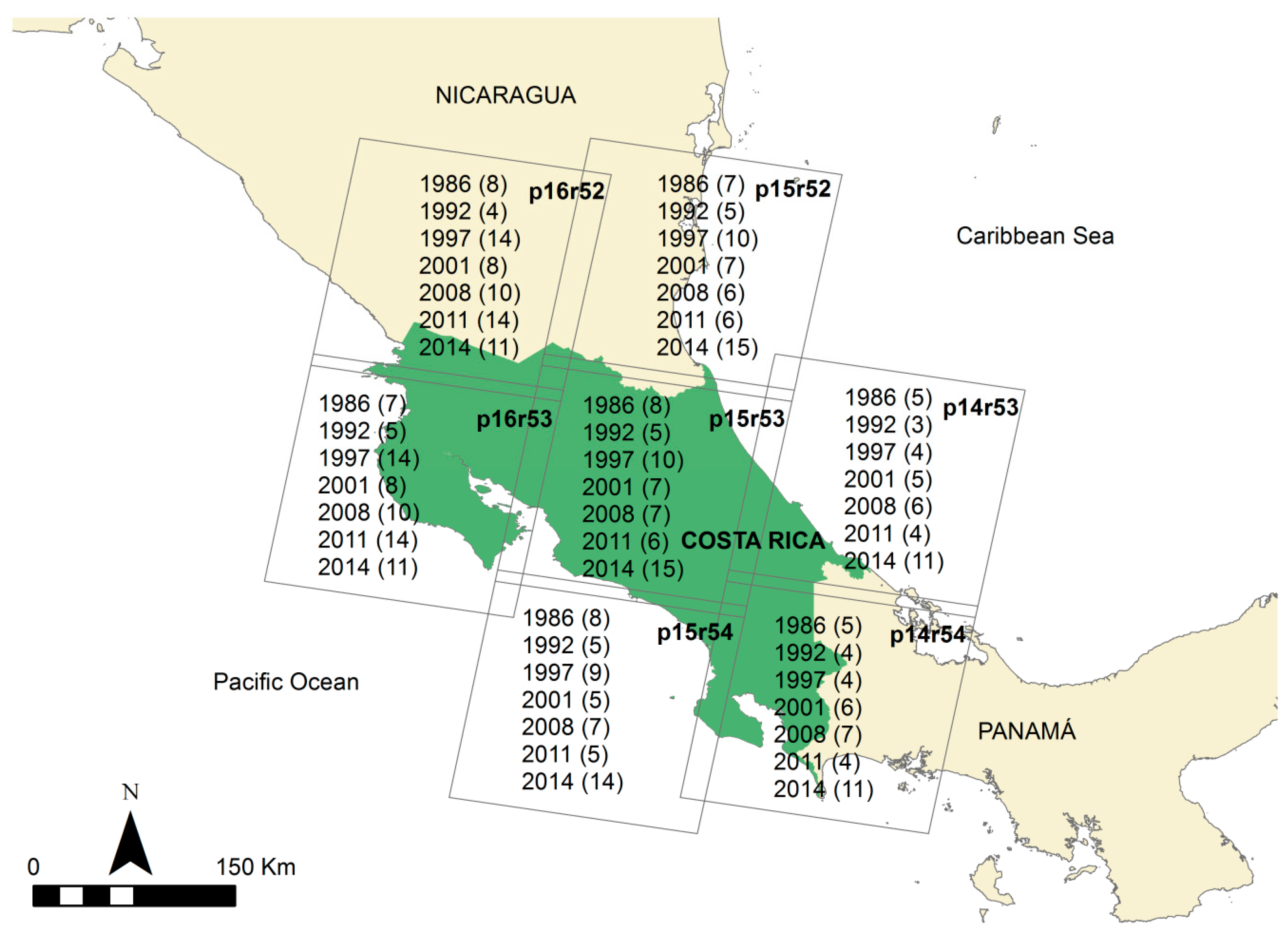
2.1. Historical Period

The choice of historical period for the design of the LC time series takes into account two major government policies and actions relative to forest conservation in Costa Rica: (1) the launch of the Payments for Environmental Services (PES) Program (23 January 1997) subsequent to the Forest law of 1996; and (2) the endorsement of Ecomercados II project by law (7 March 2008), which scaled up the PES Program significantly. Taking these temporal landmarks into account, the following years were considered in order to analyze the LC dynamics before and after their implementation: 1985/1986, 1991/1992, 1997/1998, 2000/2001, 2007/2008, 2011/2012 and 2013/2014.

2.2. Data

Full coverage of Costa Rica requires seven Landsat tiles (paths 14–16 and rows 52–54) (Figure 1). The combination of multiple images for each date and tile was necessary in order to reduce the percentage of cloud cover and cloud shadows in the final maps, yet only images within a 14 month range were considered in order to ensure temporal consistency as suggested under the Verified Carbon Standard Jurisdictional and Nested REDD+ (VCS-JNR) protocols. For this reason, the LC maps compiled data over two years (e.g., 1985/1986). A total of 384 Landsat images (30 m resolution) were used to fill the gaps caused by the abundant cloud cover and shadows: 48 from 1985/1986, 31 from 1991/1992, 65 from 1997/1998, 46 from 2000/2001, 53 from 2007/2008, 53 from 2011/2012 and 88 from 2013/2014 (Figure 1). Imagery from Landsat 4 and 5 Thematic Mapper (TM), Landsat 7 Enhanced Thematic Mapper (ETM+) and Landsat 8 Operational Land Imager and Thermal InfraRed Sensor (OLI/TIRS) were used. The images were selected between December and April (dry season) to minimize seasonal variations, except for the tiles in path 16, where some images were selected also from the rainy season to avoid confusion caused by the presence of deciduous forest.

In addition to the aforementioned Landsat satellite images, several data products were compiled in collaboration with local institutions: (i) Rapid Eye imagery (5 m resolution) from 2012 for the validation procedure of LC maps; (ii) a Digital Elevation Model (30 m resolution) from the Shuttle Radar Topography Mission (SRTM) as predictor variables; (iii) 10,000 control points with LC information from 2013 based on Rapid Eye imagery to create the training sample provided by SINAC (Conservation Area national System from Costa Rica); (iv) 21,395 control points with LC information (considered as ground reference data) for the years 1985/1986, 2000/2001 and 2013/2014 provided by INBio (National Biodiversity Institute from Costa Rica) for independent validation of the final land cover maps.

2.3. Classification Scheme

Seven individual LC maps were produced for the years 1985/1986, 1991/1992, 1997/1998, 2000/2001, 2007/2008, 2011/2012 and 2013/2014 through an open source software based workflow (Figure 2).

The LC maps for the years 1985/1986, 1991/1992 and 2000/2001 show a simplified classification scheme of two classes: forest and non-forest. The LC maps for the years 1997/1998, 2007/2008, 2011/2012 and 2013/2014 show a complete classification scheme of 12 different classes, which represents a disaggregation of the IPCC Land Use Categories (

Table 1. Comparison between the Land Use Categories considered in IPCC (2006) and the classes considered in the Land Cover (LC) Classification in Costa Rica for the years 1997/1998, 2007/2008, 2011/2012 and 2013/2014.

IPCC 2006 Class	LC Costa Rica	LC Class Description
Forest	Forest	Including also planted forests
	Mangrove	Waterlogged forest
	Palm forest	Waterlogged forest
Settlement	Settlement
Grassland	Grassland	Including anthropic pastures and natural grasslands mainly in waterlogged areas
Wetland	Water	Water bodies
Other land	Bare land
	Paramo
Cropland	Annual crops	Including rice, sugar cane and other annual crops
	Pineapple
	Coffee
	Other permanent crops	Including oil palm, orange, mango and other permanent crops

). This classification scheme was developed following the 2006 IPCC Guidelines for National Greenhouse Gas Inventories and it was agreed as part of the national REDD+ process with relevant stakeholders. In addition to these 12 LC classes, six forest age classes per forest class were obtained through a multi-temporal analysis of the maps. Forest was defined as a minimum land area of one hectare with tree crown cover of more than 30% and a minimum tree height at maturity of 5 m, in accordance with the definition stated for the Clean Development Mechanism (CDM) projects in the country.

LC change maps were produced through post-classification of individual maps, which were used to derive a LC change matrix for each of the six periods. Deforestation was defined as the transition from any of the forest to a non-forest class while forest gain was defined as the opposite transition. Forests existing since the first LC map were considered “primary forest” for this study, as it will be further discussed.

2.4. Software

Imagery preparation was completed using different open-source software. Open-source libraries and geographic information systems such as ORFEO Tool Box (OTB) [24], Geospatial Data Abstraction Library (GDAL) [25], System for Automated Geoscientific Analyses (SAGA) [26] and Geographic Resources Analysis Support System (GRASS) [27] were used through QGiS [28] processing framework. QGiS framework is a geoprocessing environment used to integrate native and third-party algorithms from QGIS. Specific tools and workflows adapted to the needs of the project were developed using Python scripts for the QGIS processing framework. In addition, R was used as the environment for statistical computing [29].

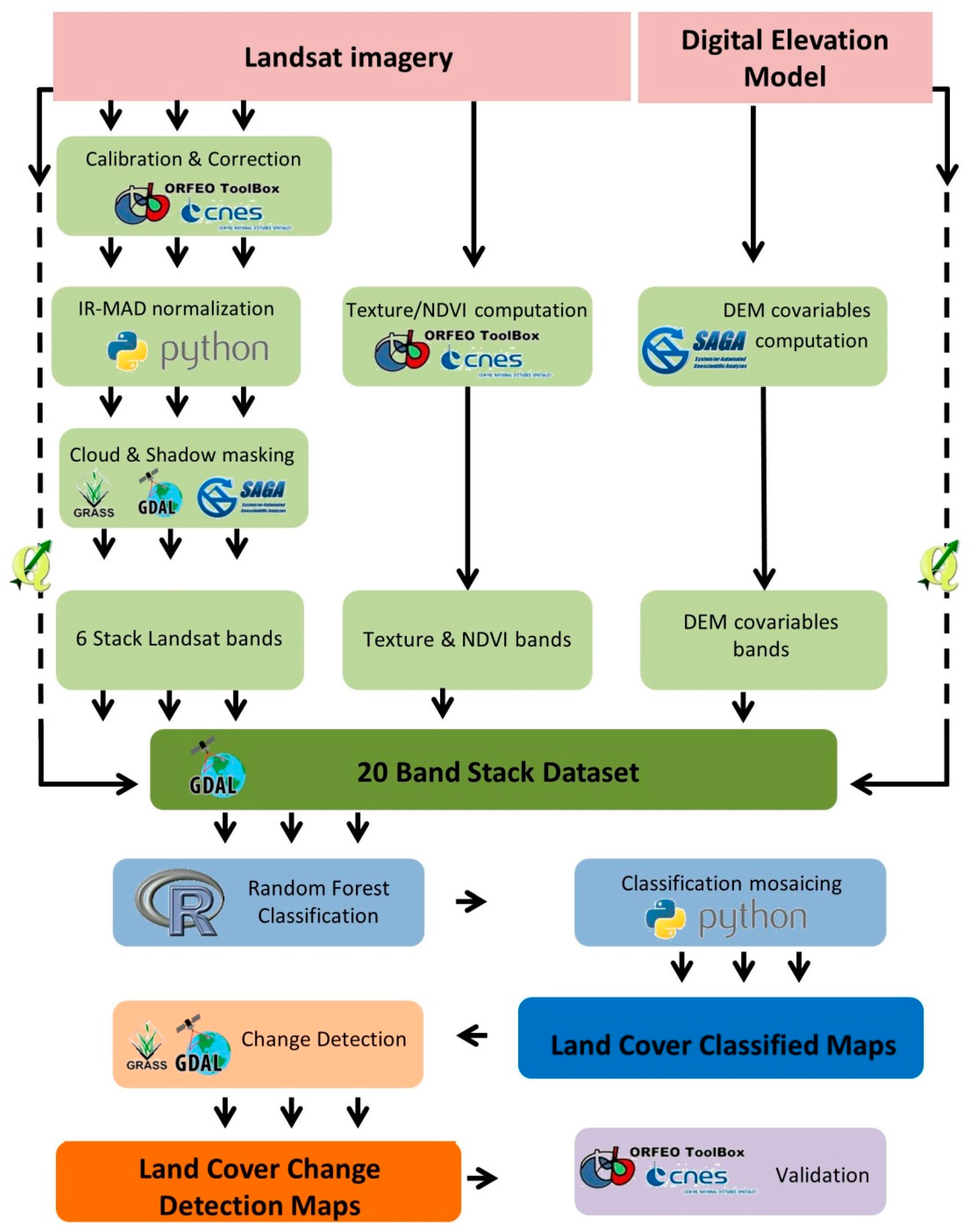
2.5. Imagery Pre-Processing

Geometric validation was firstly carried out for every single image with 20 ground control points per image. Whenever geometric correction was needed, orthorectification was carried out with the Digital Elevation Model (DEM). The radiometric calibration involved the use of standard equations to convert calibrated Digital Numbers (DN) to a satellite reflectance. Imagery were first converted to at-satellite radiance, and then to at-satellite reflectance [30]. Iteratively Re-weighted Multivariate Alteration Detection (IR-MAD) [31] was used for radiometric normalization of the images. The IR-MAD Python scripts developed by Canty [32] were integrated in QGIS. Images with the least cloud coverage were selected as reference images for the process. IR-MAD uses Canonical Correlation analysis (CCA) to find linear combinations between two groups of variables (i.e., the spectral bands of subject and reference images) to generate normalized multispectral images. This algorithm is commonly used in direct change detection approaches [31] but it has shown a good performance for radiometric normalization, avoiding the need for training the classifier for each year with specific ROIs which presents clear advantages in long term monitoring schemes.

An adaptation of the methodology from Martinuzzi et al. [33] was used for cloud and cloud shadow detection for Landsat 4, 5 and 7. For Landsat 8 images, the Quality Assessment Band was employed for cloud detection. A cloud distance map was elaborated to focus on the cloud shadow detection. Near-infrared values taking into account solar illumination and mean cloud height were used in the detection of cloud shadows. The cloud distance map consisted on a range of 4–32 pixels West and 2–27 pixels North from the cloud position. Quality control and validation of the cloud and shadow mask were done with a random point set over 18 randomly selected images. Results from the validation of the masks showed an accuracy of over 95% in the randomly sampled images.

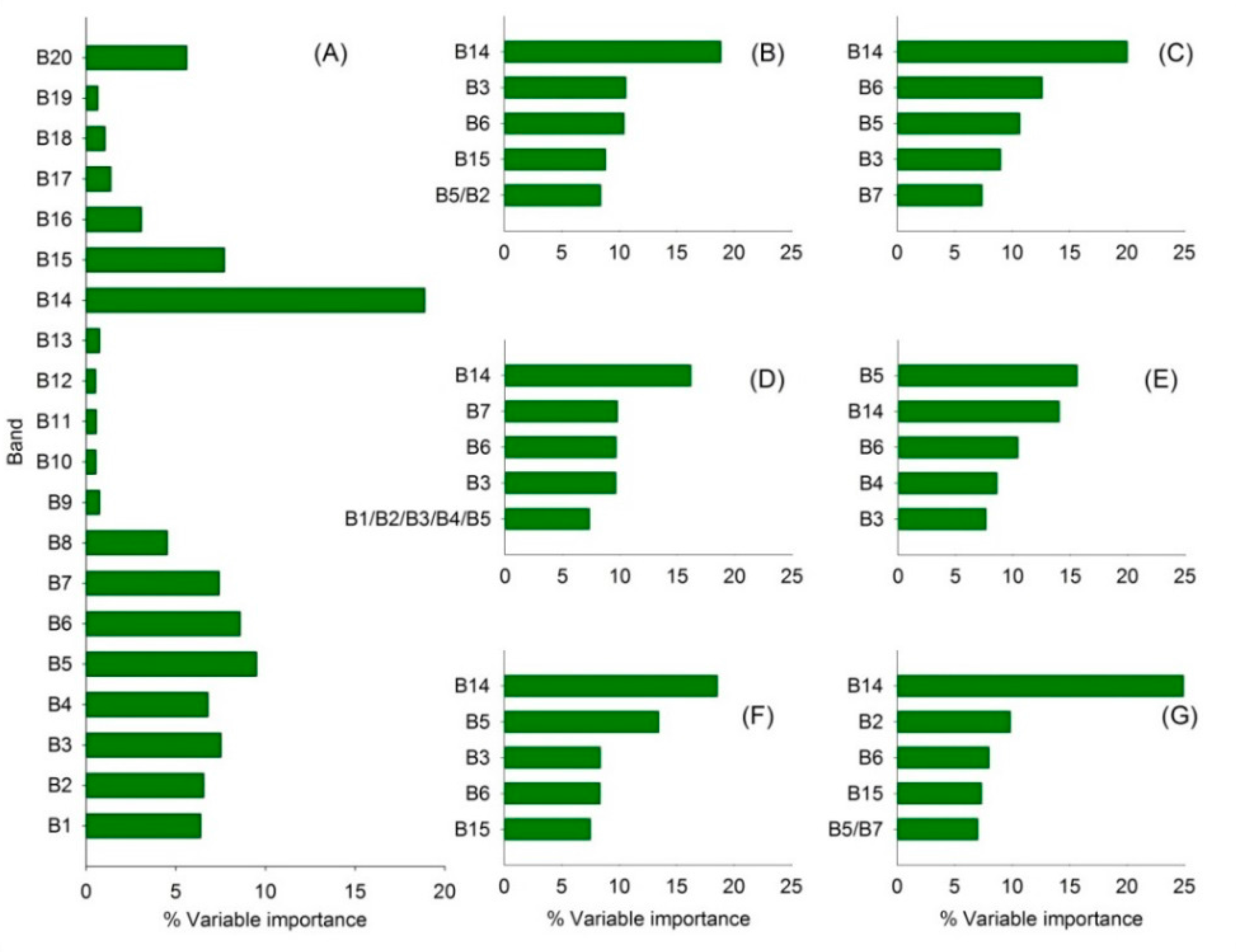
2.6. Predictor Variables

Once the set of images was pre-processed as described in the previous sections, several variables were calculated based on the spectral information of the Landsat images in order to use them as co-variates for image classification. A Normalized Difference Vegetation Index (NDVI) and different Haralick’s texture indices were computed, i.e., Mean, Sum Entropy, Difference of Entropies, Difference of Variances, IC1 and IC2 [34]. In addition, several variables were calculated based on the DEM: elevation, slope, hillshade, plan curvature, profile curvature, Convergence Index (CI) and Multiresolution Index of Valley Bottom Flatness (MRVBF) [35]. Finally, a stack of 20 bands was generated including 6 spectral bands (1–5 and 7 for Landsat 4, 5 and 7; 2–7 for Landsat 8), NDVI, 6 texture indices and 7 variable derivatives from the DEM (

Table 2. Predictor variables used in the supervised classification used to perform a Land Cover (LC) Classification in Costa Rica for the years 1985/1986, 1991/1992, 1997/1998, 2000/2001, 2007/2008, 2011/2012 and 2013/2014. Bands 1–13 are derived from Landsat images spectral data and bands 14–20 are derived from the Digital Elevation Model from the Shuttle Radar Topography Mission (STRM 30 m).

Group of Variables	Band Number	Variable
Spectral	1	Blue
	2	Green
	3	Red
	4	NIR
	5	SWIR-1
	6	SWIR-2
Vegetation Index	7	Normalized Difference Vegetation Index (NDVI)
Texture Indices	8	Mean
	9	Sum Entropy
	10	Difference of Entropies
	11	Difference of Variances
	12	IC1
	13	IC2
Digital Elevation Model	14	Elevation
	15	Slope
	16	Hillshade
	17	Plan curvature
	18	Profile curvature
	19	Convergence Index (CI)
	20	Multiresolution Index of Valley Bottom Flatness (MRVBF)

).

2.7. Image Classification

A supervised classification method was used to classify the 20 band stacks described above. The Random Forest (RF) classifier [36] was selected to perform this classification. This methodology was implemented in R, using the R package “RandomForest: Breiman and Cutler's Random Forests for classification and regression” [37], following the methodology proposed by Horning [38], modified for multiple image classification with a single algorithm. The 20 variables described above were used as explanatory co-variables in the RF models (Table 2). Random forests improve classification accuracy by growing an ensemble of classification trees and letting them vote on the classification decision. The percentage of the Random Forest decision trees voting for the final classification was computed as a classification quality factor (CQ). The classification using RF has two main steps: (i) training of the model; (ii) classifying the image using the trained classifier.

For the model training, regions of interest (ROIs) were manually defined based on (i) 10,000 control points with land cover information based on Rapid Eye imagery; (ii) high resolution historical images from Google Earth; (iii) Landsat images. These ROIs are considered as ground reference data, and they were used to adjust three different sets of models using: (i) Landsat 8 images (RF_L8 models); (ii) Landsat 5 and 7 images of the 2011/2012 and 2013/2014 dry seasons (RF_L5&7 models); and (iii) Landsat 5 and 7 images of the 2011/2012 and 2013/2014 rainy seasons, only for the NW tile (RF_L5&7_rainy model). Therefore classifiers have been adjusted using ground truth from 2011 to 2014 and have subsequently been applied to all images in the time period (from 1985 to 2014). Models RF_L8 were applied to the same Landsat 8 images used for training. The models RF_L5&7 were applied to all Landsat 5 and 7 images (from 1985 onwards) of the dry season. For the NW tile, RF_L5&7_rainy model was applied to all the other Landsat 5 and 7 images (from 1985 onwards) of the rainy season.

Mean Decrease Accuracy (MDA) was used to evaluate the importance of the variables in the RF models. For each predictor variable, MDA is the average of the accuracy across the RF minus the accuracy after permutation of the predictor. Variable importance helps identifying the most influential predictor variables in the classification of each LC class.

2.8. Post-Processing of the Classification

After classifying all 384 Landsat images with the trained RF models, classification results were composited and mosaicked in order to have a single LC map for the whole country for each year of the temporal series. The composites were produced through a specific Python tool developed ad-hoc which assigns the most suitable class to each pixel based on a measure of classification quality (CQ) given by the RF model to each class in each pixel (e.g., a pixel classified as forest in six different images and as coffee in two different images would be considered as forest, unless the sum of the CQ of every coffee classification was higher than the sum of the CQ of all the forest classifications). The compositing and mosaicking process continuously reduces clouds and clouds shadows gaps by assigning the class with the highest CQ to each pixel. The output file of the algorithm was a three band raster: (i) a band containing the classification mosaic; (ii) a band showing a measure of the RF classification quality; and (iii) a band indicating the used image to assign the class to each pixel.

Additional improvements were made to the maps via the creation of masks to increase the accuracy of the classification of some classes such as Settlements, Coffee, Paramo, Mangroves and Palm forests. These masks were based on the criteria given by local experts involved in the national REDD+ process and based on additional information such as the SINAC 2013 forest type map and the DEM. A Sieve filter of 11 pixels was applied to the final maps to establish a minimum mapping unit of 1 ha according to Costa Rica forest definition.

Despite the high number of Landsat images used per year and per tile, there were still a relatively small percentage of pixels without land cover information due to persistent cloud cover and shadows. To solve this deficiency and report a LC map without any data gap, the final LC maps for the years 2000/2001, 2007/2008, 2011/2012 and 2013/2014 were completed with land cover information from the Global Forest Change project [39]. It is important to note that the Global Forest Change project just gives information to fill the gaps based on a non-forest and forest map classes, without considering the IPCC classes used in the classification.

Post-classification LCC detection was made in order to evaluate the historical LC dynamics of Costa Rica. Based on the information of forest area in each year of the series, an estimation of forest gains and losses since 1985/1986 was generated by comparison between maps of the series.

2.9. Validation

The LC maps for the years 1985/1986, 2000/2001 and 2013/2014 were validated with external independent field data provided by the local institutions INBIO and SINAC, not used for training the classification models. A total of 5396, 7463 and 8536 points for the years 1985/1986, 2000/2001 and 2013/2014, respectively, were used for this process as valid ground reference data.

The LC change map of the period 2001–2011 was also validated. For this validation, a sampling plan was developed following the guidance set by Olofsson [40] which resulted in a sampling size of 649 points which were randomly selected and allocated to different post-stratification classes: 315 in stable forest areas, 223 stable non-forest areas, 63 in forest gain areas and 48 in deforestation areas. The ground truthing response of these points was obtained from available high resolution imagery in Costa Rica (2005 airborne photography and 2012 Rapid Eye imagery), free access high resolution database (Google Earth Digital Globe) and Landsat imagery.

Accuracy indicators for all validations were estimated using the equations and guidance provided in Olofsson [40].

3. Results

3.1. Land Cover Classification

The performed validation showed an overall accuracy of 87% for the LC map of 2013/2014 (with full legend including all the described LC classes), 93% for the 2000/2001 map (only forest/non forest classes) and 89% for the 1985/1986 map (only forest/non forest classes) (

Table 3. Validation of the Land Cover (LC) classification in Costa Rica for the years 1985/1986, 2000/2001 and 2013/2014. These dataset was mainly provided by the National Biodiversity Institute from Costa Rica (INBio) and is considered as a valid ground truth by the Government of Costa Rica.

Validation Year	Overall Accuracy	Land Cover Class	Producer’s Accuracy	User’s Accuracy
1985/1986	0.89	Forest	0.89	0.91
		No-forest	0.88	0.85
2000/2001	0.93	Forest	0.92	0.94
		No-forest	0.94	0.92
2013/2014	0.87	Forest	0.91	0.91
		Palm forest	0.68	0.99
		Mangrove forest	0.97	0.91
		Settlement	0.99	0.92
		Grassland	0.85	0.76
		Paramo	0.94	0.85
		Water	0.97	0.60
		Bare land	0.19	0.58
		Annual crops	0.81	0.88
		Pineapple	0.88	0.93
		Other permanent crops (including coffee)	0.82	0.93

). These overall accuracy values are within the range indicated by GOFC-GOLD [10].

The most important variable in the classification (Figure 3) is elevation (B14), followed by the spectral variables (from B1 to B7) and slope (B15). The MRVBF (B20) and one of the texture variables (B8) also contributed to a lesser extent to the classification, while the importance of the remaining variables was small compared to the former (Figure 3). However, the relative importance of these variables in the classification varies depending on each class (Figure 3). Regarding the spectral bands (from B1 to B7) and slope (B15), it can also be observed how the relative importance of these variables fluctuate depending on each class, e.g., the SWIR-1 band (B5) turned out to be a very important variable for classifying grassland and coffee and its importance was lower in other classes such as forest, waterlogged forests, settlement or pineapple, while slope (B15) was moderately important for classifying forest, coffee or pineapple and its importance was lower in other classes such as grasslands, settlement or waterlogged forests (Figure 3).

Despite the high number of Landsat images processed and classified in each year of the time series, a small percentage of pixels remained without classification due to clouds and shadows (Figure 4). However, this percentage is less than 2% of the country for every year in the series.

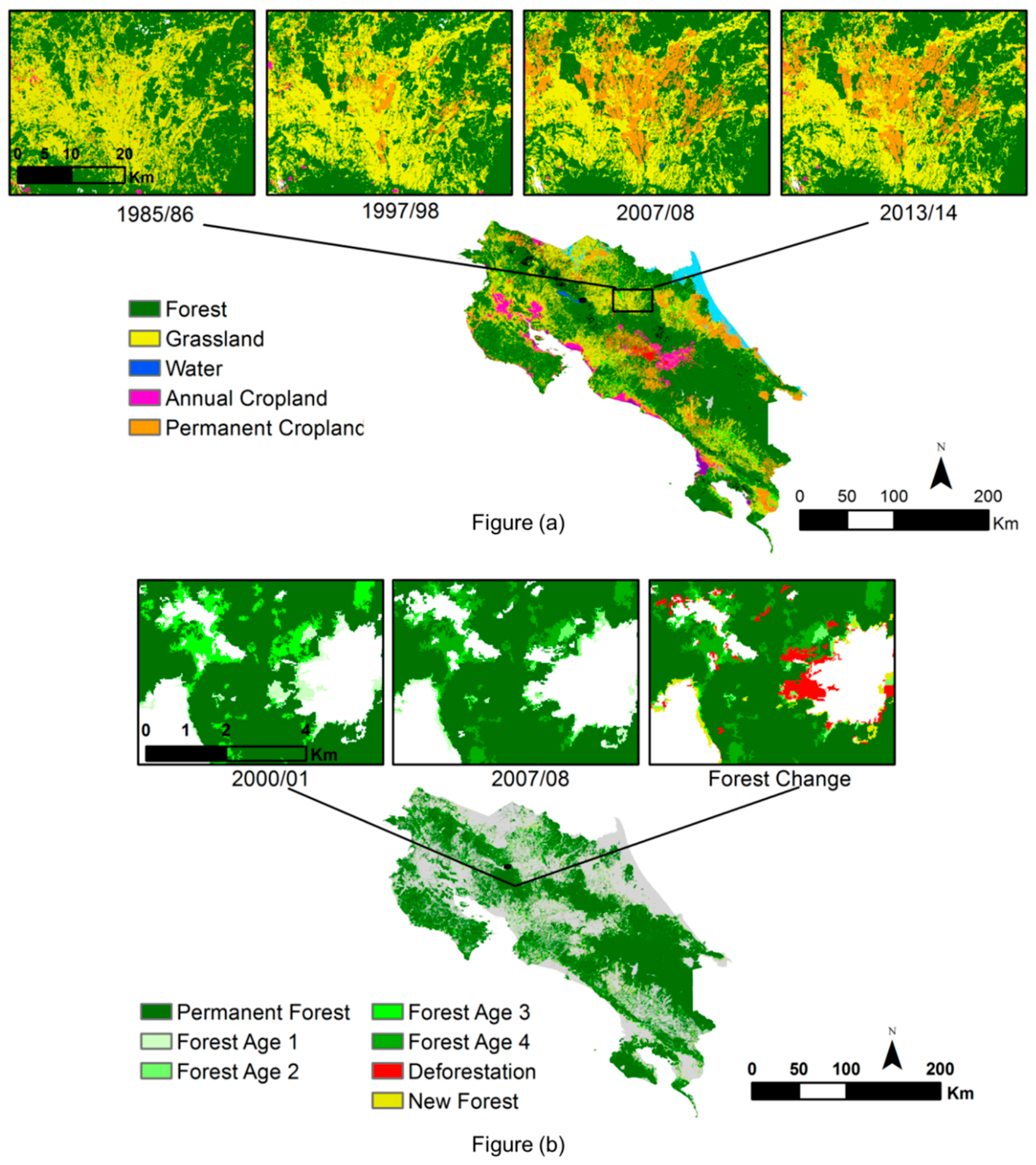
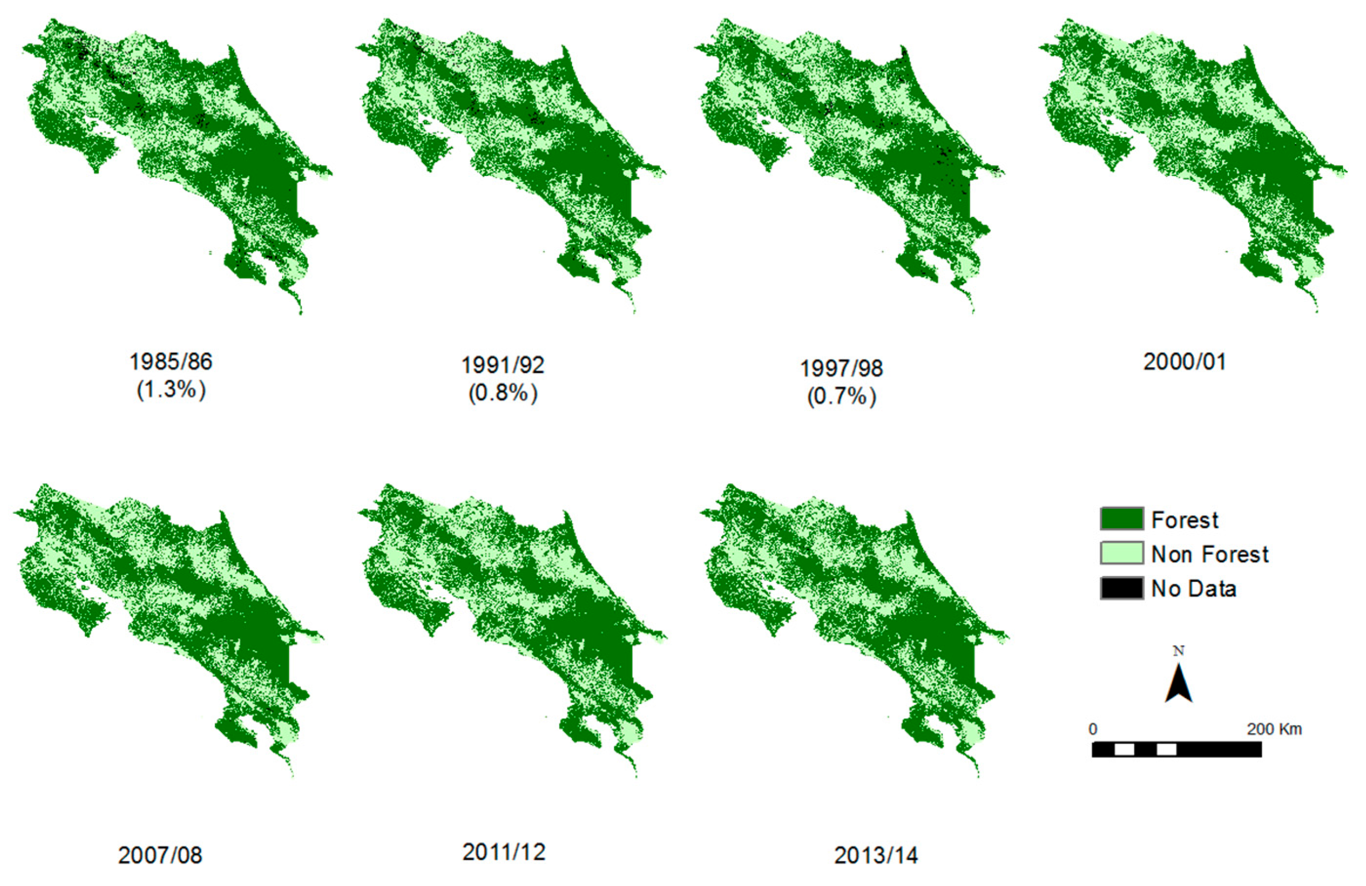
3.2. Land Cover Change Detection

Forest cover changes were validated for the period 2001–2011, with an overall accuracy of 86% (

Table 4. Validation of the observed Land Cover Changes in Costa Rica between 2001 and 2011. The validation was done using the methodology proposed by Olofsson [40] and it is based on 649 randomly selected control points. Confidence intervals (95% significance level) of the accuracy values are reported in parenthesis.

Change Classes	Description	Producer’s Accuracy (Omission)	User’s Accuracy (Commission)	Overall Accuracy
Deforestation	Forest to Non-Forest	0.49 (0.36–0.62)	0.62 (0.47–0.77)	0.86 (0.83–0.89)
Afforestation/reforestation	Non-Forest to Forest	0.50 (0.38–0.62)	0.75 (0.62–0.88)
Forest (no change)	Forest remaining Forest	0.95 (0.93–0.97)	0.88 (0.84–0.91)
Non-forest (no change)	Non-Forest remaining Non-Forest	0.84 (0.8–0.88)	0.87 (0.83–0.92)

). Even though this result may be considered as satisfactory, there is a noticeable difference between the accuracy in forest and non-forest stable classes (87%–88% user accuracy) and the forest change classes (62%–75% user accuracy) (Table 4). LC and LCC areas for the entire historical time series are specified in the Costa Rica Forest Reference Emission Level available at the Forest Carbon Partnership Facility (FCPF).

Forest age-classes were estimated through a multi-temporal analysis of the maps. Age classes vary according to the time difference between the maps. The elapsed time since the appearance of forest in a pixel allows assigning the forest age-class to each forest pixel of the maps (

Table 5. Forest age computed for the time series dataset since 1985/1986. Forest age classes show different age per period due to different time period lengths.

Forest Change Detection Period	1991	1997	2000	2007	2011	2013
1986–1991	1–6	7–12	13–15	16–22	23–26	27–28
1992–1997		1–6	7–9	10–16	17–20	21–22
1998–2000			1–3	4–10	11–14	15–16
2001–2007				1–7	8–11	12–13
2008–2011					1–4	5–6
2012–2013						1–2

). Forests remaining as forests are ascending in age-class in each study period, so a forest age-class area can be compared with the subsequent age-class area in the following study period (e.g., forest age class 1 in 1991/1992 would correspond with forest age class 2 in 1997/1998).

4. Discussion

4.1. Land Cover Classification

The usefulness of classifiers based on decision trees, e.g., data mining tools C5 classifier developed by Quinlan [41], had already been discussed for Costa Rica, as they allow the incorporation of spectral information together with a variety of other variables such as textural bands and DEM derivatives, among others [42,43]. The incorporation of global no charge for user DEM, as Aster Global Elevation Map which is more recent and with highest resolution or Sentinel imagery from mission Copernicus, would help improve the final results in further research. The classifications performed as part of the present paper were based on the Random Forest models, which are nowadays considered as the most efficient tool for adjusting these kinds of models [12,44,45,46,47,48]. The good performance of RF in this LC analysis at a national scale reinforces the evidence for the high potential of this tool to perform operational classification tasks [12]. This is especially relevant considering that RF is a free open source classifier which can be easily used in a free open source environment such as R. Indeed, the performed LC was fully implemented using free open source software (ORFEO, GDAL, SAGA, GRASS, QGIS and R), pointing out the capability of these tools for the operational implementation of this kind of LC tasks at a national level, handling a high number of images, as it has been previously shown [12]. Different free tools such as the available set for temporal data processing in GRASS are also interesting alternatives to include in the workflow to LC and LCC maps at the national scale.

Although the models were only trained for 2011/2012 and 2013/2014 imagery, the validated performance of the model over 2000/2001 and 1985/1986 imagery shows the effectiveness of the normalization process with the IR–MAD algorithm. Ground truth LC datasets might do not exist when generating a long historical series, especially for the oldest periods of these series. However, large amount of high quality data is usually available in recent years. Therefore, the most recent and complete available field information is used in the adjustment and validation processes. Our methodology allows generating a long historical LC series even though ground truth is only available for a few periods of the series.

The high relevance of elevation in LC has been previously described by other authors [12,48,49,50]. In a country such as Costa Rica, with an elevation range of 0–3819 m in an area of just 51,100 km², elevation plays a key role in the arrangement of land cover in the landscape and it has been traditionally observed as a determinant ecological variable and a proxy for several other environmental variables such as precipitation and temperature [51]. Landsat SWIR-1 band (2nd most important variable in the present study, Figure 3) has also been previously identified as a key variable for LC, associated with its vegetation and soil moisture sensitivity properties [12]. Moisture sensitivity was an important factor in the present study because Landsat imagery was selected from the dry period and, consequently, different land covers situated in different landscape positions maintain different moisture levels. Indeed, the SWIR-1 band was the most relevant variable for grassland determination (Figure 3) which explains the inclusion within this grassland class of many wetlands with grassland vegetation.

Obtaining close-to-cloud-free LC maps for every year of the series is considered as one of the biggest accomplishments of the present study and one of the keystones of the proposed methodology. Clouds represent a significant inconvenient in humid tropical regions such as Costa Rica [33] and achieving a cloud-free LC is important in the REDD+ context in order to comply with the principle of completeness.

The remaining low proportion of data gaps caused by the permanent presence of clouds and shadows could be then filled with data from global products. Global Forest Change project [39] was used in the present case, but others global projects can be also used, such as the Global Forest/Non Forest map from ALOS Palsar mosaics [52].

4.2. Land Cover Change Detection

Although post-classification LCC detection has some limitations (due to errors propagation) compared to direct LCC detection, post-classification was selected due to the need of mapping large number of classes in each LC and LCC maps. The methodology presented allows knowing the LC class after deforestation that permits more accurate estimations of GHG emissions from land use and land use change.

The six Forest age-classes obtained through the multi-temporal analysis of the series (Table 5) allows for accurately assigning forest age in each period thereby reducing the area considered as “primary forest” along the series. This is useful for assigning more accurate emission factors to deforested areas and to assign more accurate removal factors to young secondary forests as well as modeling future rates of carbon emissions and removals. This methodology is feasible due to the large number of available study periods. Some limitations arise nevertheless from the hypothesis to determine the first age-class as forest areas in the first year (1985/1986) of the series as “primary forest” (Table 5) as it is likely that forests in 1985/1986 include significant areas of secondary forests which resulted from forests regenerated in the 80s as a consequence of the cattle crisis [53]. Therefore, some of the deforestation detected over these “primary forests” would eventually occur over these young secondary forests. This limitation can be mitigated by dividing the areas classified as forest in the first year of the time series (1985/1986) into “primary” and “secondary” forest. For the subsequent construction of FRELs/FRLs, this division was performed based on an auxiliary map with areas of secondary forest in 1978–1980 elaborated by the National Meteorological Institute of Costa Rica.

The complexity to separate primary and older secondary forest is a common limitation in all remote sensing temporal series of LC change. The shorter the time series, the greater the influence of the potential limitation would be. A short temporal series generates a lower age-class range and therefore a less accurate estimation of emissions and removals, e.g., assuming as “primary forest” all forests from 2000/2001 is less accurate than assuming forest from 1985/1986 as “primary forest”.

By linking deforestation dynamics with forest age, a more accurate description of the process of LCC and associated GHG emissions along the time series can be presented. Figure 5b shows an example of the spatial distribution of age classes and deforestation processes, pointing out that these processes occur mainly along the border of areas of “primary forests” and in areas of young secondary forests. Deforestation of young secondary forests is the dominant land-use change process in the time series (Figure 5b). This provides a new understanding of deforestation processes in the context of REDD+ initiatives in Costa Rica. Emission factors of young secondary forests are lower than those of older or primary forests and accounting for this difference is critical for the construction of a credible FRELs/FRLs and posterior MRV. Moreover, forest age classes could be used to help define when regenerated vegetation is considered as forest, either according to the definition of “forest” under REDD+ or according to the legal definition of “forest”. In Costa Rica, the relationship between vegetation age and diameter at breast height (dbh) of the trees (trees of more than 15 cm dbh according to the Forest Law No. 7575) could be used to assess whether an area with new woody vegetation is already a “forest” according to the Forest Law. Grassland-fallow dynamics in Costa Rica illustrates this situation. Clearing recently forested land before it reaches the thresholds at which it is considered ‘‘forest’’ is a common practice among landowners to avoid the ban on forest clearing under the aforementioned law [21]. This clearing of young forest age-classes that is detected in our results (Figure 5b) has been documented in Costa Rica before [17] and it is considered one of the most common patterns of LC dynamics in the country.

A challenge for Costa Rica, and possibly for other countries as well, is that the parameters and thresholds used to define “forest” under the national legislation are different of those used in the context of REDD+ and the national GHG inventory. Defining a minimum forest age class could thus help finding a definition of “deforestation” that is consistent with the Law and applicable in the context of REDD+, helping also to determine the periodicity required in order for future monitoring events to appropriately assess deforestation events.

Additionally, the spatial pattern of different forest age classes obtained through this time series (e.g., Figure 5b) allows complementary studies of secondary forest fragmentation, which has been identified as a key issue in deforestation and forest regeneration studies in the region [43,53,54].

In countries like Costa Rica, where a large proportion of the forests are secondary forests, the study of a long historical period to assess LC and LCC is critical for assessing the distribution of age classes in forested areas and to generate more accurate estimates of emissions from deforestation. Our study covers a historical period of nearly 30 years and includes seven LC maps. Although the historical period considered for establishing the national FRELs/FRLs is usually around 10 years, the analysis of a longer period is critical for avoiding an over-estimation of emissions from deforestation. This is especially important in tropical areas where the fast growth of vegetation enables a rapid recuperation of forest cover detectable in satellite images, although the carbon content of young secondary forests may take decades and even centuries to equal the carbon content of primary forests.

The ample number of LC classes allows for improving the study of deforestation drivers in a spatial explicitly model. The comparison of LC maps clearly shows the dynamics of land cover in Costa Rica in the last 28 years, e.g., pineapple crops expansion in the last decades over former forest or grassland areas (Figure 5a). This information can be used for the interconnection and complementarity of monitoring efforts for different initiatives in the national greenhouse gas emissions framework, such as Nationally Appropriate Mitigation Actions (NAMAs) in the agriculture or other sectors and the National REDD+ Strategy.

The high comparability of Landsat images and the use of a single classification model for all years ensures strong consistency among the generated historical LC maps, which is considered a mandatory requirement for this kind of analysis within the REDD+ context [7].

5. Conclusions

A methodology for generating consistent data for the establishment of a historical time series and subsequent monitoring of LC dynamics, based on Landsat imagery and open-source software is presented here and tested as a valid operational framework in the context of the REDD+ mechanism. The good validation results for both LC and LC change maps confirms the capability of Random Forest, R package, QGIS and other free open source software (ORFEO, GDAL, SAGA, GRASS, QGIS and R) for the implementation of LC classification maps, which can lower the costs of this kind of projects within the REDD+ context for many developing countries.

An almost cloud-free LC map for every year of the time series was obtained by combining a large number of images. The procedure presented in this paper overcomes the inconvenience of dense cloud cover recurrent in humid tropical regions, without additional costs. Therefore, the usage of a worldwide open access imagery database such as Landsat allows for filling the gaps originating from clouds and cloud shadow removal, representing a cost-effective and replicable methodology with high relevance for developing countries in the context of REDD+.

The usage of the IR-MAD algorithm in image normalization provides consistency in the composition of single image classification and to the entire time series of activity data from LCC allowing for the application of the same trained machine learning algorithm across the entire period of the series.

Due to the requirement of mapping a large number of LC and LCC classes, post-classification LCC detection was selected instead of direct change detection. Although having a large number of LC and LCC classes is a clear advantage for this study, the lower accuracy of deforestation and reforestation mapping shows the need for improving post-classification LCC methodologies to increase the accuracy, reducing error propagation.

In addition, this study shows the advantages of obtaining forest age classes from long time series of activity data. Forest age classes allow improving the assessment of secondary regeneration according to the forest definition applied and for a more accurate estimation of GHG emissions when deforestation is assessed.

References

1. Angelsen, A.; McNeill, D. Evolution of REDD. In Analysing REDD+: Challenges and Choices; Angelsen, A., Brockhaus, M., Sunderlin, W.D., Verchot, L.V., Eds.; Center for International Forestry Research: Bogor Barat, Indonesia, 2012; pp. 31–51. [Google Scholar]
2. Angelsen, A.; Brockhaus, M.; Sunderlin, W.D.; Verchot, L.V. Analysing REDD: Challenges and Choices; Center for International Forestry Research (CIFOR): Bogor, Indonesia, 2012. [Google Scholar]
3. UNFCCC. Report of the Conference of the Parties on its Seventeenth Session; Decision 12/CP.17, Durban, 28 November to 11 December 2011; UNFCC: Bonn, Germany, 2011. [Google Scholar]
4. UNFCCC. Methodological Guidance for Activities Relating to Reducing Emissions from Deforestation and Forest Degradation and the Role of Conservation, Sustainable Management of Forests and Enhancement of Forest Carbon Stocks in Developing Countries; Decision 4/CP.15, UN Doc FCCC/CP/2009/11/Add.1 (30 March 2010); UNFCCC: Bonn, Germany, 2010. [Google Scholar]
5. De Sy, V.; Herold, M.; Achard, F.; Asner, G.P.; Held, A.; Kellndorfer, J.; Verbesselt, J. Synergies of multiple remote sensing data sources for REDD monitoring. Curr. Opin. Environ. Sustain. 2012, 4, 696–706. [Google Scholar] [CrossRef]
6. Joseph, S.; Herold, M.; Sunderlin, W.D.; Verchot, L.V. REDD readiness: Early insights on monitoring, reporting and verification systems of project developers. Environ. Res. Lett. 2013, 8, 034038. [Google Scholar] [CrossRef]
7. Korhonen-Kurki, K.; Brockhaus, M.; Duchelle, A.E.; Atmadja, S.; Thuy, P.T. Multiple levels and multiple challenges for REDD. In Analysing REDD 2012; Center for International Forestry Research (CIFOR): Bogor, Indonesia, 2012; Volume 91. [Google Scholar]
8. UNFCCC. Cost of Implementing Methodologies and Monitoring Systems Relating to Estimates of Emissions from Deforestation and Forest Degradation, the Assessment of Carbon Stocks and Greenhouse Gas Emissions from Changes in Forest Cover, and the Enhancement of Forest Carbon Stocks; Technical Paper FCCC/TP/2009/1; UNFCCC: Bonn, Germany, 2009. [Google Scholar]
9. Hansen, M.C.; Loveland, T.R. A review of large area monitoring of land cover change using Landsat data. Remote Sens. Environ. 2012, 122, 66–74. [Google Scholar] [CrossRef]
10. GOFC-GOLD. A Sourcebook of Methods and Procedures for Monitoring and Reporting Anthropogenic Greenhouse Gas Emissions and Removals Associated with Deforestation, Gains and Losses of Carbon Stocks in Forests Remaining Forests, and Forestation; GOFC-GOLD Land Cover Project Office: Wageningen University, The Netherlands, 2013; p. 236. [Google Scholar]
11. Vittek, M.; Brink, A.; Donnay, F.; Simonetti, D.; Desclée, B. Land cover change monitoring using Landsat MSS/TM satellite image data over West Africa between 1975 and 1990. Remote Sens. 2014, 6, 658–676. [Google Scholar] [CrossRef] [Green Version]
12. Mellor, A.; Haywood, A.; Stone, C.; Jones, S. The performance of random forests in an operational setting for large area sclerophyll forest classification. Remote Sens. 2013, 5, 2838–2856. [Google Scholar] [CrossRef]
13. Barton, D.N.; Faith, D.; Rusch, G.; Acevedo, H.; Paniagua, L.; Castro, M. Environmental service payments: Evaluating biodiversity conservation trade-offs and cost-efficiency in the Osa Conservation Area, Costa Rica. J. Environ. Manag. 2009, 90, 901–911. [Google Scholar] [CrossRef] [PubMed]
14. Daniels, A.E.; Bagstad, K.; Esposito, V.; Moulaert, A.; Rodriguez, C.M. Understanding the impacts of Costa Rica’s PES: Are we asking the right questions? Ecol. Econ. 2010, 69, 2116–2126. [Google Scholar] [CrossRef]
15. Fagan, M.; DeFries, R.; Sesnie, S.; Arroyo, J.; Walker, W.; Soto, C.; Chazdon, R.; Sanchun, A. Land cover dynamics following a deforestation ban in northern Costa Rica. Environ. Res. Lett. 2013, 8, 034017. [Google Scholar] [CrossRef]
16. Kalacska, M.; Sanchez-Azofeifa, G.A.; Rivard, B.; Calvo-Alvarado, J.C.; Quesada, M. Baseline assessment for environmental services payments from satellite imagery: A case study from Costa Rica and Mexico. J. Environ. Manag. 2008, 88, 348–359. [Google Scholar] [CrossRef] [PubMed]
17. Morse, W.C.; Schedlbauer, J.L.; Sesnie, S.E.; Finegan, B.; Harvey, C.A.; Hollenhorst, S.J.; Kavanagh, K.L.; Stoian, D.; Wulfhorst, J. Consequences of environmental service payments for forest retention and recruitment in a Costa Rican biological corridor. Ecol. Soc. 2009, 14, 23. [Google Scholar]
18. Sanchez-Azofeifa, G.A.; Rivard, B.; Calvo, J.; Moorthy, I. Dynamics of tropical deforestation around national parks: Remote sensing of forest change on the Osa Peninsula of Costa Rica. Mt. Res. Dev. 2002, 22, 352–358. [Google Scholar] [CrossRef]
19. Sanchez-Azofeifa, A.; Pfaff, A.; Robalino, J.A.; Boomhower, J.P. Costa Rica’s payment for environmental services program: intention, implementation, and impact. Conserv. Biol. 2007, 21, 1165–1173. [Google Scholar] [CrossRef] [PubMed]
20. Sánchez-Azofeifa, G.A.; Harriss, R.C.; Skole, D.L. Deforestation in Costa Rica: A quantitative analysis using remote sensing imagery. Biotropica 2001, 33, 378–384. [Google Scholar] [CrossRef]
21. Sierra, R.; Russman, E. On the efficiency of environmental service payments: a forest conservation assessment in the Osa Peninsula, Costa Rica. Ecol. Econ. 2006, 59, 131–141. [Google Scholar] [CrossRef]
22. Pontius, R.G.; Cornell, J.D.; Hall, C.A. Modeling the spatial pattern of land-use change with GEOMOD2: Application and validation for Costa Rica. Agric. Ecosyst. Environ. 2001, 85, 191–203. [Google Scholar] [CrossRef]
23. FONAFIFO. Estudio de Cobertura Forestal de Costa Rica; Cooperación Financiera Costa Rica—Alemania: San José, Costa Rica, 2012. [Google Scholar]
24. OTB Development Team. ORFEO Tool Box. Centre National d’Études Spatiales; CNES: Paris, France, 2013. [Google Scholar]
25. GDAL. GDAL—Geospatial Data Abstraction Library; Open Source Geospatial Foundation: Beaverton, OR, USA, 2015. [Google Scholar]
26. Conrad, O.; Bechtel, B.; Bock, M.; Dietrich, H.; Fischer, E.; Gerlitz, L.; Wehberg, J.; Wichmann, V.; Böhner, J. System for Automated Geoscientific Analyses (SAGA) version 2.1.4. Geosci. Mod. Dev. 2015, 8, 1991–2007. [Google Scholar] [CrossRef]
27. GRASS Development Team. Geographic Resources Analysis Support System (GRASS) Software; Version 7.0; Open Source Geospatial Foundation: Beaverton, OR, USA, 2015. [Google Scholar]
28. QGIS Development Team. QGIS Geographic Information System; v 2.4; Open Source Geospatial Foundation: Beaverton, OR, USA, 2009. [Google Scholar]
29. R Development Core Team. R 2.4.0; R Foundation for Statistical Computing: Vienna, Austria, 2006. [Google Scholar]
30. Chander, G.; Markham, B.L.; Helder, D.L. Summary of current radiometric calibration coefficients for Landsat MSS, TM, ETM, and EO-1 ALI sensors. Remote Sens. Environ. 2009, 113, 893–903. [Google Scholar] [CrossRef]
31. Canty, M.J.; Nielsen, A.A. Automatic radiometric normalization of multitemporal satellite imagery with the iteratively re-weighted MAD transformation. Remote Sens. Environ. 2008, 112, 1025–1036. [Google Scholar] [CrossRef]
32. Canty, M.J. Image Analysis, Classification and Change Detection in Remote Sensing: With Algorithms for ENVI/IDL and Python; CRC Press: Boca Raton, FL, USA, 2014. [Google Scholar]
33. Martinuzzi, S.; Gould, W.A.; González, O.M.R. Creating Cloud-Free Landsat ETM Data Sets in Tropical Landscapes: Cloud and cloud-Shadow Removal; US Department of Agriculture, Forest Service, International Institute of Tropical Forestry Río Piedras: San Juan, Puerto Rico, 2007.
34. Haralick, R.M. Statistical and structural approaches to texture. Proc. IEEE 1979, 67, 786–804. [Google Scholar] [CrossRef]
35. Gallant, J.C.; Dowling, T.I. A multiresolution index of valley bottom flatness for mapping depositional areas. Water Resour. Res. 2003, 39. [Google Scholar] [CrossRef]
36. Breiman, L. Random forests. Mach. Learn. 2001, 45, 5–32. [Google Scholar] [CrossRef]
37. Liaw, A.; Wiener, M. Classification and regression by randomForest. R News 2002, 2/3, 18–22. [Google Scholar]
38. Horning, N. Introduction to Decision Trees and Random Forests; American Museum of Natural History’s Center for Biodiversity and Conservation: New York, NY, USA, 2013. [Google Scholar]
39. Hansen, M.C.; Potapov, P.V.; Moore, R.; Hancher, M.; Turubanova, S.A.; Tyukavina, A.; Thau, D.; Stehman, S.V.; Goetz, S.J.; Loveland, T.R.; et al. High-resolution global maps of 21st-century forest cover change. Science 2013, 342, 850–853. [Google Scholar] [CrossRef] [PubMed]
40. Olofsson, P.; Foody, G.M.; Herold, M.; Stehman, S.V.; Woodcock, C.E.; Wulder, M.A. Good practices for estimating area and assessing accuracy of land change. Remote Sens. Environ. 2014, 148, 42–57. [Google Scholar] [CrossRef]
41. Quinlan, J.R. C4. 5: Programs for Machine Learning; Morgan Kaufmann: San Mateo, CA, USA, 1993. [Google Scholar]
42. Sesnie, S.E.; Gessler, P.E.; Finegan, B.; Thessler, S. Integrating Landsat TM and SRTM-DEM derived variables with decision trees for habitat classification and change detection in complex neotropical environments. Remote Sens. Environ. 2008, 112, 2145–2159. [Google Scholar] [CrossRef]
43. Algeet-Abarquero, N.; Sánchez-Azofeifa, A.; Bonatti, J.; Marchamalo, M. Land cover dynamics in Osa Region, Costa Rica: Secondary forest is here to stay. Reg. Environ. Chang. 2014. [Google Scholar] [CrossRef]
44. Pal, M. Random forest classifier for remote sensing classification. Int. J. Remote Sens. 2005, 26, 217–222. [Google Scholar] [CrossRef]
45. Gislason, P.O.; Benediktsson, J.A.; Sveinsson, J.R. Random forests for land cover classification. Pattern Recog. Lett. 2006, 27, 294–300. [Google Scholar] [CrossRef]
46. Waske, B.; Braun, M. Classifier ensembles for land cover mapping using multitemporal SAR imagery. ISPRS J. Photogramm. Remote Sens. 2009, 64, 450–457. [Google Scholar] [CrossRef]
47. Ghimire, B.; Rogan, J.; Galiano, V.R.; Panday, P.; Neeti, N. An evaluation of bagging, boosting, and random forests for land-cover classification in Cape Cod, Massachusetts, USA. GiSci. Remote Sens. 2012, 49, 623–643. [Google Scholar] [CrossRef]
48. Rodriguez-Galiano, V.F.; Ghimire, B.; Rogan, J.; Chica-Olmo, M.; Rigol-Sanchez, J.P. An assessment of the effectiveness of a random forest classifier for land-cover classification. ISPRS J. Photogramm. Remote Sens. 2012, 67, 93–104. [Google Scholar] [CrossRef]
49. Fahsi, A.; Tsegaye, T.; Tadesse, W.; Coleman, T. Incorporation of digital elevation models with Landsat-TM data to improve land cover classification accuracy. For. Ecol. Manag. 2000, 128, 57–64. [Google Scholar] [CrossRef]
50. Dewan, A.M.; Yamaguchi, Y. Land use and land cover change in Greater Dhaka, Bangladesh: Using remote sensing to promote sustainable urbanization. Appl. Geogr. 2009, 29, 390–401. [Google Scholar] [CrossRef]
51. Holdridge, L.R. Life Zone Ecology; Tropical Science Center: San Jose, Costa Rica, 1967. [Google Scholar]
52. Shimada, M.; Itoh, T.; Motooka, T.; Watanabe, M.; Shiraishi, T.; Thapa, R.; Lucas, R. New global forest/non-forest maps from ALOS PALSAR data (2007–2010). Remote Sens. Environ. 2014, 155, 13–31. [Google Scholar] [CrossRef]
53. Arroyo-Mora, J.P.; Sánchez-Azofeifa, G.A.; Rivard, B.; Calvo, J.C.; Janzen, D.H. Dynamics in landscape structure and composition for the Chorotega region, Costa Rica from 1960 to 2000. Agric. Ecosyst. Environ. 2005, 106, 27–39. [Google Scholar] [CrossRef]
54. Broadbent, E.N.; Zambrano, A.M.A.; Dirzo, R.; Durham, W.H.; Driscoll, L.; Gallagher, P.; Salters, R.; Schultz, J.; Colmenares, A.; Randolph, S.G. The effect of land use change and ecotourism on biodiversity: A case study of Manuel Antonio, Costa Rica, from 1985 to 2008. Landsc. Ecol. 2012, 27, 731–744. [Google Scholar] [CrossRef]
Figure 1. Details of the number of Landsat images processed for each year of the time series and each of the 7 Landsat tiles which covers Costa Rica: paths (p) 14–16, rows (r) 52–54.
Remotesensing 08 00593 g001
Figure 2. Methodological workflow for land cover and land cover change classification.
Remotesensing 08 00593 g002
Figure 3. Measurement of the relative variable importance of the predictor variables in the adjusted Random Forests for classifying: (A) complete land cover classification; (B) forest class; (C) palm forest classes; (D) settlement class; (E) grassland class; (F) pineapple class; (G) coffee class.
Remotesensing 08 00593 g003
Figure 4. Distribution of the forest and non-forest land cover classes in Costa Rica for every year of the temporal series (1985/1986, 1991/1992, 1997/1998, 2000/2001, 2007/2008, 2011/2012 and 2013/2014). Details about the percent of the country where no class could be assigned due to clouds and shadows are reported in parenthesis. There are not gaps due to cloud and cloud shadows for the years 2000/2001, 2007/2008, 2011/2012 and 2013/2014. For the remainder of the years, gaps without information were filled using land cover information from the Global Forest Change project [39].
Remotesensing 08 00593 g004
Figure 5. Illustration of land cover change dynamics in sample areas in Costa Rica: (a) Permanent cropland expansion from 1986 to 2013; (b) Forest age class distribution and deforestation patterns over different forest age classes.
Remotesensing 08 00593 g005