
Exploring the Relationship between Burn Severity Field Data and Very High Resolution GeoEye Images: The Case of the 2011 Evros Wildfire in Greece


Abstract
:
1. Introduction
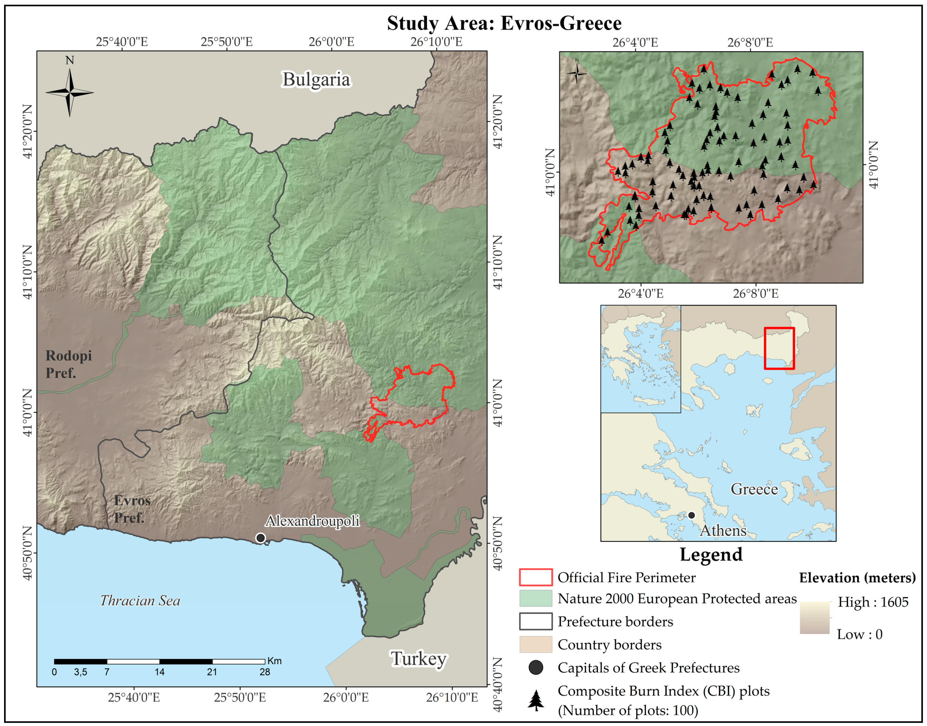
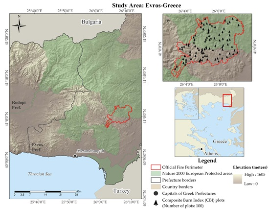
2. Study Area
3. Datasets and Preprocessing
3.1. Field Data
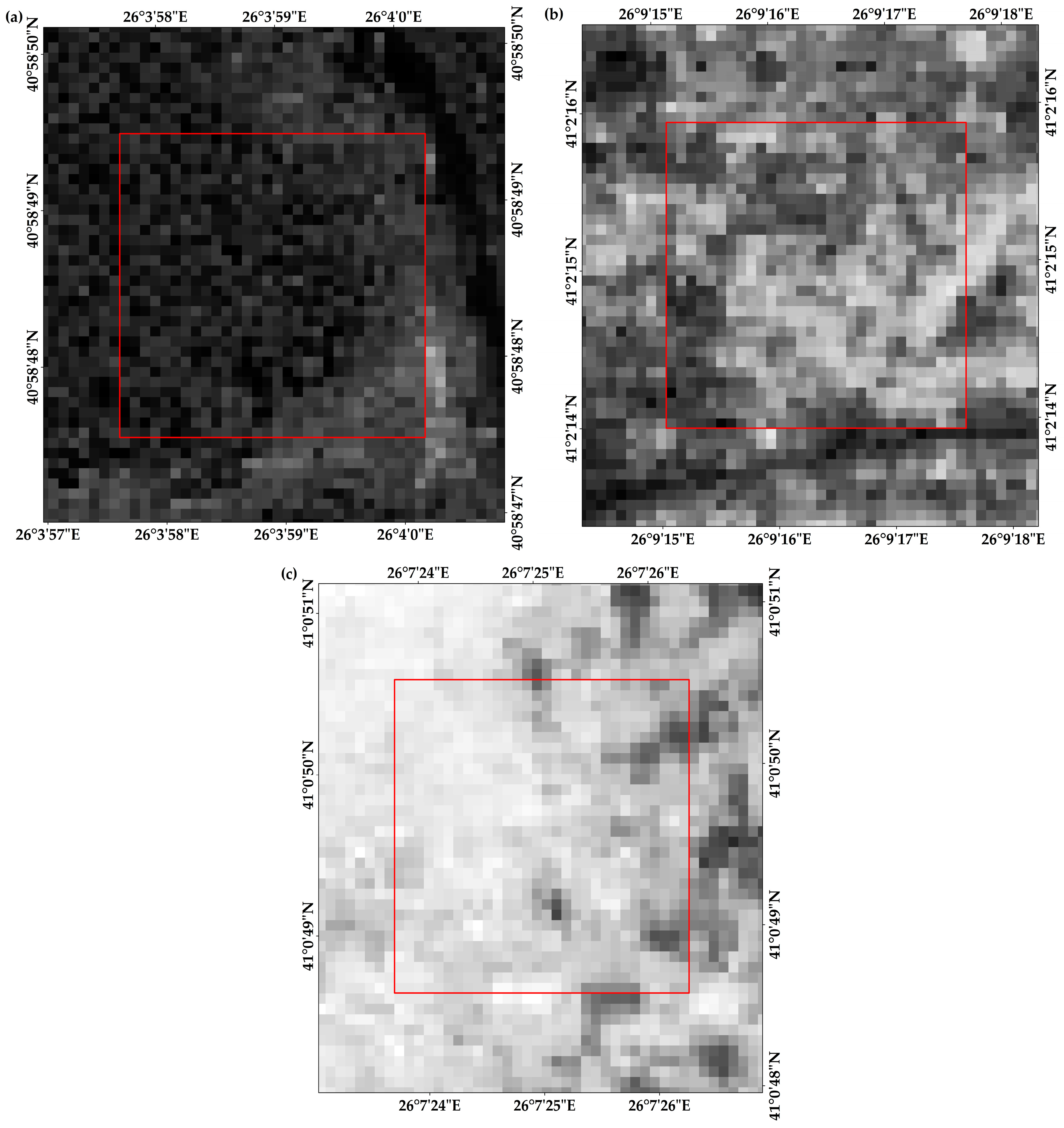
3.2. Satellite Data
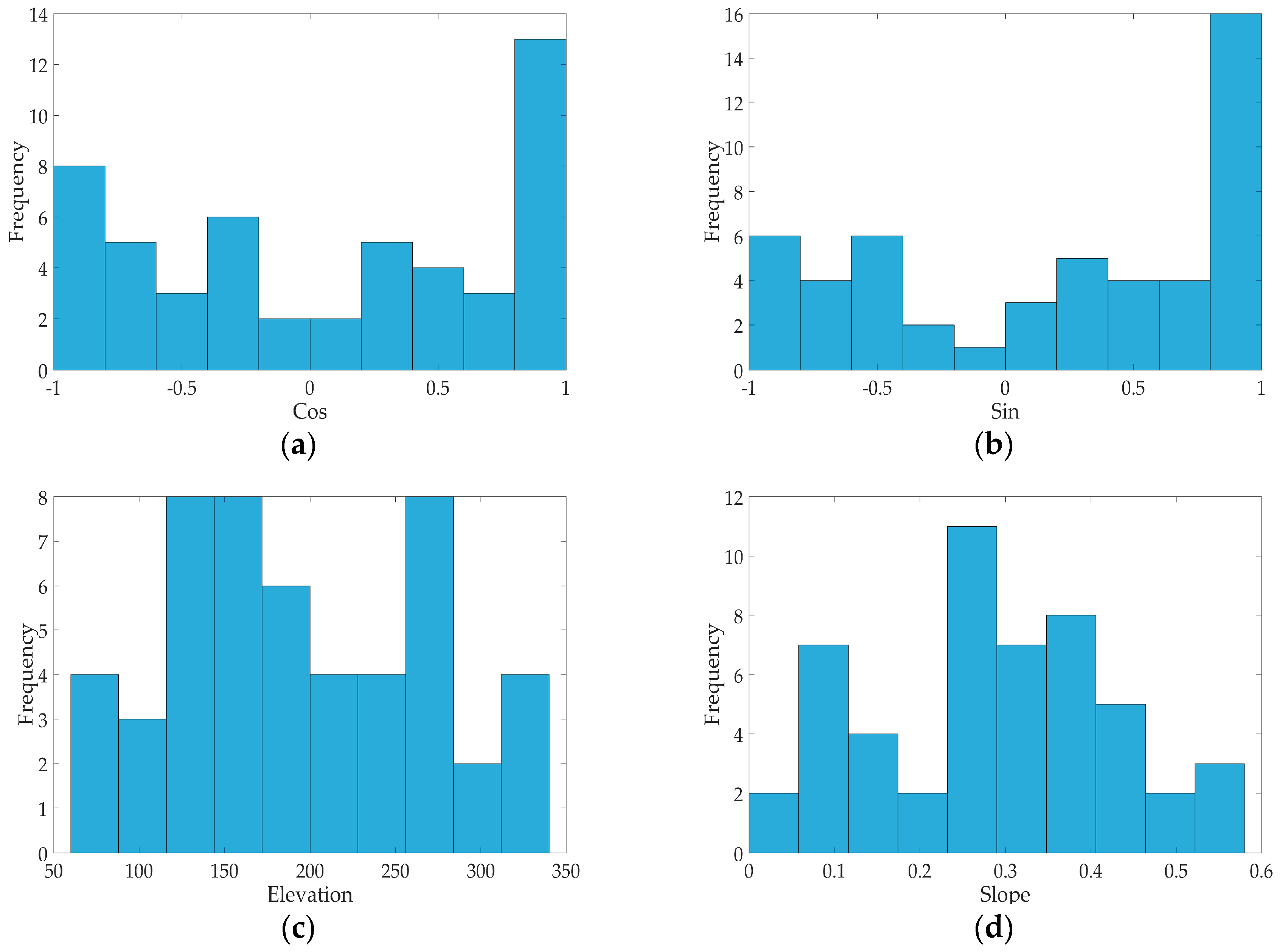
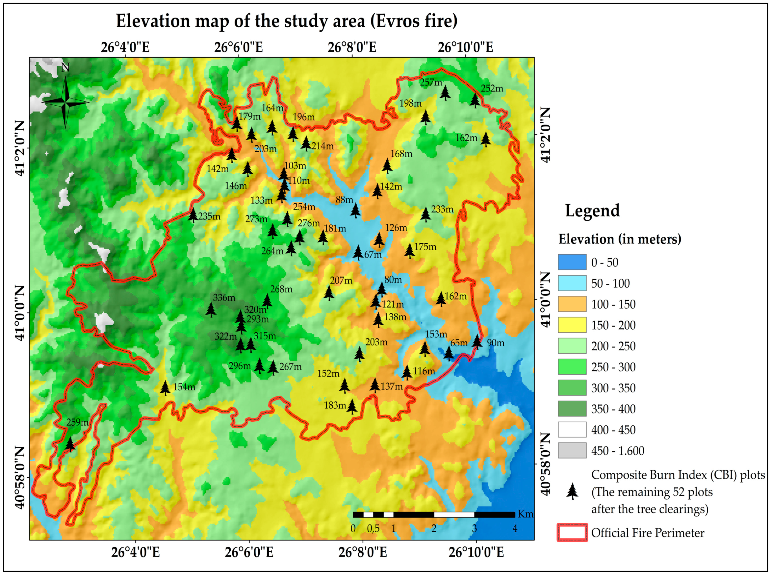
3.3. Topographic Data
4. Methodology
5. Results
6. Discussion
7. Conclusions
Acknowledgments
Author Contributions
Conflicts of Interest
References
- Moreira, F.; Viedma, O.; Arianoutsou, M.; Curt, T.; Koutsias, N.; Rigolot, E.; Barbati, A.; Corona, P.; Vaz, P.; Xanthopoulos, G. Landscape-wildfire interactions in southern Europe: Implications for landscape management. J. Environ. Manag. 2011, 92, 2389–2402. [Google Scholar] [CrossRef] [PubMed] [Green Version]
- Hoscilo, A.; Tansey, K.J.; Page, S.E. Post-fire vegetation response as a proxy to quantify the magnitude of burn severity in tropical peatland. Int. J. Remote Sens. 2013, 34, 412–433. [Google Scholar] [CrossRef]
- Lentile, L.B.; Holden, Z.A.; Smith, A.M.; Falkowski, M.J.; Hudak, A.T.; Morgan, P.; Lewis, S.A.; Gessler, P.E.; Benson, N.C. Remote sensing techniques to assess active fire characteristics and post-fire effects. Int. J. Wildland Fire 2006, 15, 319–345. [Google Scholar] [CrossRef]
- Gouveia, C.; DaCamara, C.; Trigo, R. Post-fire vegetation recovery in Portugal based on spot/vegetation data. Nat. Hazards Earth Syst. Sci. 2010, 10, 673–684. [Google Scholar] [CrossRef]
- Chen, X.; Vogelmann, J.E.; Rollins, M.; Ohlen, D.; Key, C.H.; Yang, L.; Huang, C.; Shi, H. Detecting post-fire burn severity and vegetation recovery using multitemporal remote sensing spectral indices and field-collected composite burn index data in a ponderosa pine forest. Int. J. Remote Sens. 2011, 32, 7905–7927. [Google Scholar] [CrossRef]
- FAO. State of the World’s Forests-2014; FAO: Rome, Italy, 2014. [Google Scholar]
- Gitas, I.; Polychronaki, A.; Mitri, G.; Veraverbeke, S. Advances in Remote Sensing of Post-Fire Vegetation Recovery Monitoring—A Review; InTech: Vienna, Austria, 2012. [Google Scholar]
- Key, C.H.; Benson, N.C. Landscape assessment (LA). In FIREMON: Fire Effects Monitoring and Inventory System; General Technical Report RMRS-GTR-164-CD; Rocky Mountain Research Station, US Department of Agriculture, Forest Service: Fort Collins, CO, USA, 2006; pp. LA-1–LA-51. [Google Scholar]
- Birch, D.S.; Morgan, P.; Kolden, C.A.; Abatzoglou, J.T.; Dillon, G.K.; Hudak, A.T.; Smith, A.M. Vegetation, topography and daily weather influenced burn severity in central Idaho and western Montana forests. Ecosphere 2015, 6, 1–23. [Google Scholar] [CrossRef]
- Naveh, Z. Mediterranean uplands as anthropogenic perturbation dependent systems and their dynamic conservation management. In Terrestrial and Aquatic Ecosystems, Perturbation and Recovery; Ellis Horwood: New York, NY, USA, 1991; pp. 544–556. [Google Scholar]
- Ryan, K.C. Dynamic interactions between forest structure and fire behavior in boreal ecosystems. Silva Fenn. 2002, 36, 13–39. [Google Scholar] [CrossRef]
- Schepers, L.; Haest, B.; Veraverbeke, S.; Spanhove, T.; Vanden Borre, J.; Goossens, R. Burned area detection and burn severity assessment of a heathland fire in Belgium using Airborne Imaging Spectroscopy (APEX). Remote Sens. 2014, 6, 1803–1826. [Google Scholar] [CrossRef]
- Ireland, G.; Petropoulos, G.P. Exploring the relationships between post-fire vegetation regeneration dynamics, topography and burn severity: A case study from the Montane Cordillera Ecozones of Western Canada. Appl. Geogr. 2015, 56, 232–248. [Google Scholar] [CrossRef]
- Catry, F.; Rego, F.; Moreira, F.; Fernandes, P.; Pausas, J. Post-fire tree mortality in mixed forests of central Portugal. For. Ecol. Manag. 2010, 260, 1184–1192. [Google Scholar] [CrossRef]
- Driscoll, D.A.; Lindenmayer, D.B.; Bennett, A.F.; Bode, M.; Bradstock, R.A.; Cary, G.J.; Clarke, M.F.; Dexter, N.; Fensham, R.; Friend, G. Fire management for biodiversity conservation: Key research questions and our capacity to answer them. Biol. Conserv. 2010, 143, 1928–1939. [Google Scholar] [CrossRef]
- Moreira, F.; Arianoutsou, M.; Vallejo, V.R.; de las Heras, J.; Corona, P.; Xanthopoulos, G.; Fernandes, P.; Papageorgiou, K. Setting the scene for post-fire management. In Post-Fire Management and Restoration of Southern European Forests; Springer: Berlin, Germany; Heidelberg, Germany, 2012; pp. 1–19. [Google Scholar]
- Viedma, O.; Quesada, J.; Torres, I.; De Santis, A.; Moreno, J.M. Fire severity in a large fire in a Pinus pinaster forest is highly predictable from burning conditions, stand structure, and topography. Ecosystems 2014, 18, 237–250. [Google Scholar] [CrossRef]
- Morgan, P.; Keane, R.E.; Dillon, G.K.; Jain, T.B.; Hudak, A.T.; Karau, E.C.; Sikkink, P.G.; Holden, Z.A.; Strand, E.K. Challenges of assessing fire and burn severity using field measures, remote sensing and modelling. Int. J. Wildland Fire 2014, 23, 1045–1060. [Google Scholar] [CrossRef]
- Karaman, M.; Özelkan, E.; Örmeci, C. Determination of the forest fire potential by using remote sensing and geographical information system, case study-Bodrum/Turkey. In Advances in Remote Sensing and GIS Applications in Forest Fire Management From Local to Global Assessments; Publications office of the European Union: Stressa, Italy, 2011; pp. 51–55. [Google Scholar]
- Collins, B.M.; Kelly, M.; van Wagtendonk, J.W.; Stephens, S.L. Spatial patterns of large natural fires in Sierra Nevada wilderness areas. Landsc. Ecol. 2007, 22, 545–557. [Google Scholar] [CrossRef]
- Turner, M.G.; Hargrove, W.W.; Gardner, R.H.; Romme, W.H. Effects of fire on landscape heterogeneity in Yellowstone National Park, Wyoming. J. Veg. Sci. 1994, 731–742. [Google Scholar] [CrossRef]
- Pinto, A.; Fernandes, P.M. Microclimate and modeled fire behavior differ between adjacent forest types in Northern Portugal. Forests 2014, 5, 2490–2504. [Google Scholar] [CrossRef]
- Boiffin, J.; Aubin, I.; Munson, A.D. Ecological controls on post-fire vegetation assembly at multiple spatial scales in eastern North American boreal forests. J. Veg. Sci. 2014. [Google Scholar] [CrossRef]
- Mouillot, F.; Ratte, J.-P.; Joffre, R.; Mouillot, D.; Rambal, S. Long-term forest dynamic after land abandonment in a fire prone Mediterranean landscape (central Corsica, France). Landsc. Ecol. 2005, 20, 101–112. [Google Scholar] [CrossRef]
- Key, C.; Benson, N. Measuring and remote sensing of burn severity. In Proceedings of the Joint Fire Science Conference and Workshop, Boise, Idaho, 15–17 June 1999; p. 284.
- Key, C.; Benson, N. FIREMON: Fire Effects Monitoring and Inventory System; USDA Forest Service, Rocky Mountain Research Station: Fort Collins, CO, USA, 2006. [Google Scholar]
- Chuvieco, E. Earth Observation of Wildland Fires in Mediterranean Ecosystems; Springer: Berlin/Heidelberg, Germany, 2009. [Google Scholar]
- Keeley, J.E. Fire intensity, fire severity and burn severity: A brief review and suggested usage. Int. J. Wildland Fire 2009, 18, 116–126. [Google Scholar] [CrossRef]
- Mitri, G.H.; Gitas, I.Z. Mapping the severity of fire using object-based classification of IKONOS imagery. Int. J. Wildland Fire 2008, 17, 431–442. [Google Scholar] [CrossRef]
- Amato, V.J.; Lightfoot, D.; Stropki, C.; Pease, M. Relationships between tree stand density and burn severity as measured by the Composite Burn Index following a ponderosa pine forest wildfire in the American Southwest. For. Ecol. Manag. 2013, 302, 71–84. [Google Scholar] [CrossRef]
- Chen, G.; Metz, M.R.; Rizzo, D.M.; Dillon, W.W.; Meentemeyer, R.K. Object-based assessment of burn severity in diseased forests using high-spatial and high-spectral resolution MASTER airborne imagery. ISPRS J. Photogramm. Remote Sens. 2015, 102, 38–47. [Google Scholar] [CrossRef]
- Keane, R.E.; Dillon, G.; Jain, T.; Hudak, A.; Morgan, P.; Karau, E.; Sikkink, P.; Silverstein, R. The Problems with Fire Severity and Its Application in Fire Management; USDA Forest Service, Rocky Mountain Research Station: Missoula, MT, Canada, 2012. [Google Scholar]
- Díaz-Delgado, R.; Lloret, F.; Pons, X. Influence of fire severity on plant regeneration by means of remote sensing imagery. Int. J. Remote Sens. 2003, 24, 1751–1763. [Google Scholar] [CrossRef]
- Edwards, A.C.; Maier, S.W.; Hutley, L.B.; Williams, R.J.; Russell-Smith, J. Spectral analysis of fire severity in north Australian tropical savannas. Remote Sens. Environ. 2013, 136, 56–65. [Google Scholar] [CrossRef]
- Dzwonko, Z.; Loster, S.; Gawroński, S. Impact of fire severity on soil properties and the development of tree and shrub species in a Scots pine moist forest site in southern Poland. For. Ecol. Manag. 2015, 342, 56–63. [Google Scholar] [CrossRef]
- Wang, G.G.; Kemball, K.J. The effect of fire severity on early development of understory vegetation following a stand-replacing wildfire. In Proceedings of the 5th Symposium on Fire and Forest Meteorology Jointly with 2nd International Wildland Fire Ecology and Fire Management Congress, Orlando, FL, USA, 16–20 November 2003; pp. 16–20.
- Johnstone, J.F.; Chapin, F.S., III. Effects of soil burn severity on post-fire tree recruitment in boreal forest. Ecosystems 2006, 9, 14–31. [Google Scholar] [CrossRef]
- Blaschke, T.; Hay, G.J.; Kelly, M.; Lang, S.; Hofmann, P.; Addink, E.; Feitosa, R.Q.; van der Meer, F.; van der Werff, H.; van Coillie, F. Geographic object-based image analysis—Towards a new paradigm. ISPRS J. Photogramm. Remote Sens. 2014, 87, 180–191. [Google Scholar] [CrossRef] [PubMed]
- Cansler, C.A.; McKenzie, D. How robust are burn severity indices when applied in a new region? Evaluation of alternate field-based and remote-sensing methods. Remote Sens. 2012, 4, 456–483. [Google Scholar] [CrossRef]
- Demirel, N.; Emil, M.K.; Duzgun, H.S. Surface coal mine area monitoring using multi-temporal high-resolution satellite imagery. Int. J. Coal Geol. 2011, 86, 3–11. [Google Scholar] [CrossRef]
- Epting, J.; Verbyla, D. Landscape-level interactions of prefire vegetation, burn severity, and postfire vegetation over a 16-year period in interior Alaska. Can. J. For. Res. 2005, 35, 1367–1377. [Google Scholar] [CrossRef]
- Tucker, C.J. Red and photographic infrared linear combinations for monitoring vegetation. Remote Sens. Environ. 1979, 8, 127–150. [Google Scholar] [CrossRef]
- Casady, G.M.; van Leeuwen, W.J.; Marsh, S.E. Evaluating post-wildfire vegetation regeneration as a response to multiple environmental determinants. Environ. Model. Assess. 2010, 15, 295–307. [Google Scholar] [CrossRef]
- Wu, Z.; Middleton, B.; Hetzler, R.; Vogel, J.; Dye, D. Vegetation burn severity mapping using Landsat-8 and WorldView-2. Photogramm. Eng. Remote Sens. 2015, 81, 143–154. [Google Scholar] [CrossRef]
- Deng, Y.; Goodchild, M.F.; Chen, X. Using NDVI to define thermal south in several mountainous landscapes of California. Comput. Geosci. 2009, 35, 327–336. [Google Scholar] [CrossRef]
- Wimberly, M.C.; Reilly, M.J. Assessment of fire severity and species diversity in the southern Appalachians using Landsat TM and ETM+ imagery. Remote Sens. Environ. 2007, 108, 189–197. [Google Scholar] [CrossRef]
- Dillon, G.K.; Holden, Z.A.; Morgan, P.; Crimmins, M.A.; Heyerdahl, E.K.; Luce, C.H. Both topography and climate affected forest and woodland burn severity in two regions of the western US, 1984 to 2006. Ecosphere 2011, 2, 1–33. [Google Scholar] [CrossRef]
- Rao, C.R. The use and interpretation of principal component analysis in applied research. In Sankhyā: The Indian Journal of Statistics, Series A; Springer: Berlin, Germany; Heidelberg, Germany, 1964; pp. 329–358. [Google Scholar]
- Legendre, P.; Legendre, L.F. Numerical Ecology; Elsevier: Amsterdam, The Netherlands, 2012. [Google Scholar]
- Legendre, P.; Oksanen, J.; ter Braak, C.J. Testing the significance of canonical axes in redundancy analysis. Methods Ecol. Evol. 2011, 2, 269–277. [Google Scholar] [CrossRef]
- Gittins, R. Canonical Analysis: A Review with Applications in Ecology; Springer: Berlin, Germany; Heidelberg, Germany, 1985. [Google Scholar]
- Van den Brink, P.J.; ter Braak, C.J. Principal response curves: Analysis of time-dependent multivariate responses of biological community to stress. Environ. Toxicol. Chem. 1999, 18, 138–148. [Google Scholar] [CrossRef]
- Bajocco, S.; Rosati, L.; Ricotta, C. Knowing fire incidence through fuel phenology: A remotely sensed approach. Ecol. Model. 2010, 221, 59–66. [Google Scholar] [CrossRef]
- Ter Braak, C.J.; Prentice, I.C. A theory of gradient analysis. Adv. Ecol. Res. 1988, 18, 271–317. [Google Scholar]
- Legendre, P.; Legendre, L. Numerical Ecology, 2nd ed.; Elsevier: Amsterdam, The Netherlands, 1998. [Google Scholar]


| Satellite Sensor | Code Name | Acquisition Date | Spectral Range |
|---|---|---|---|
| GeoEye-1 | GeoEyetime1 | 20 November 2011 | Blue: 450–510 nm |
| Green: 510–580 nm | |||
| Red: 655–690 nm | |||
| Near Infra Red: 780–920 nm | |||
| GeoEye-1 | GeoEyetime2 | 23 August 2012 | Blue: 450–510 nm |
| Green: 510–580 nm | |||
| Red: 655–690 nm | |||
| Near Infra Red: 780–920 nm | |||
| WorldView-2 | - | Soon after the fire | Blue: 450–510 nm |
| Green: 510–580 nm | |||
| Red: 630–690 nm | |||
| Near Infra Red 1: 770–895 nm |
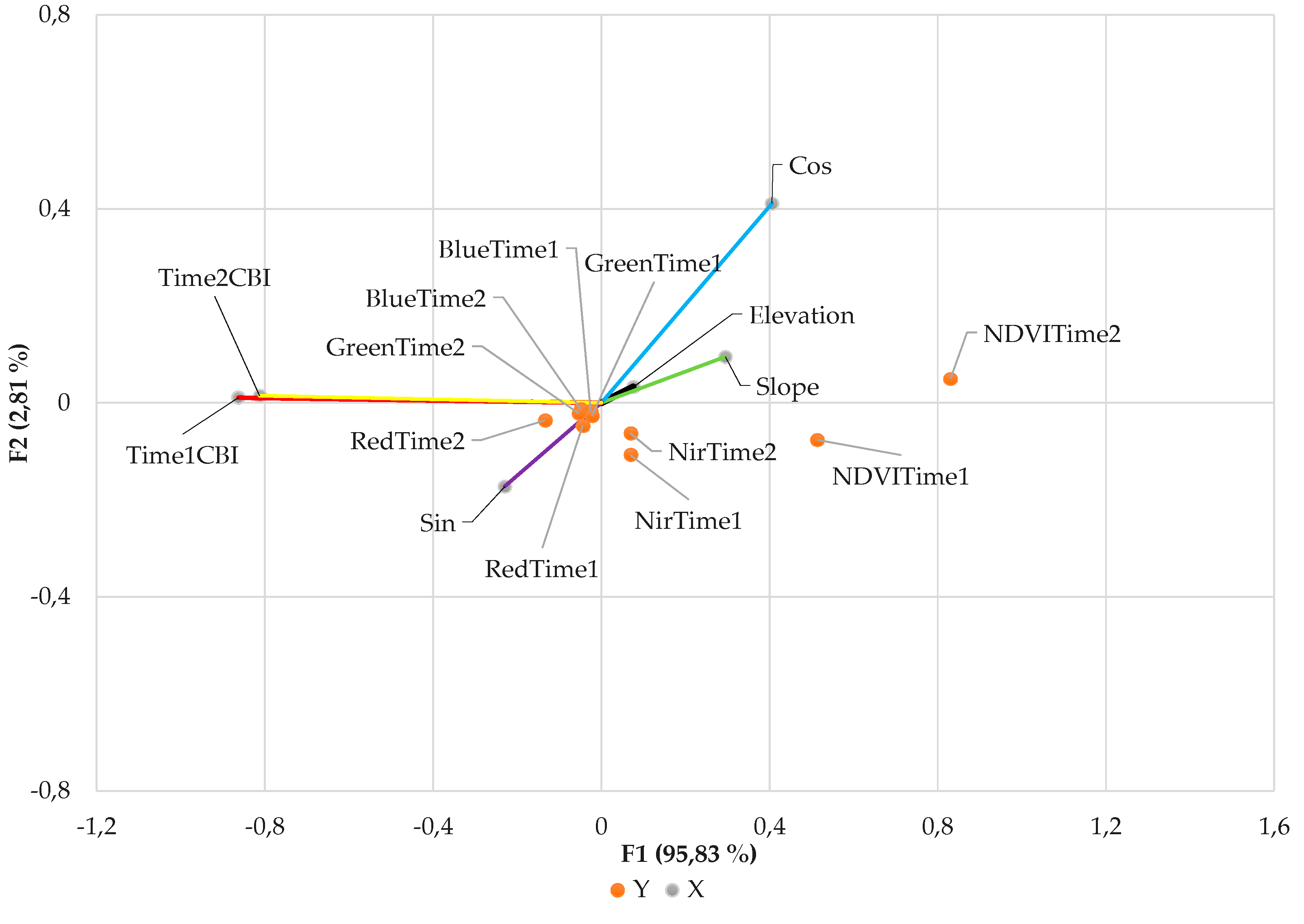
| Variable | F1 | F2 | F3 |
|---|---|---|---|
| Elevation | 0.0764 | 0.0328 | −0.4437 |
| Slope | 0.2954 | 0.0949 | 0.0787 |
| Cos | 0.4058 | 0.4115 | −0.0962 |
| Sin | −0.2299 | −0.1725 | −0.2778 |
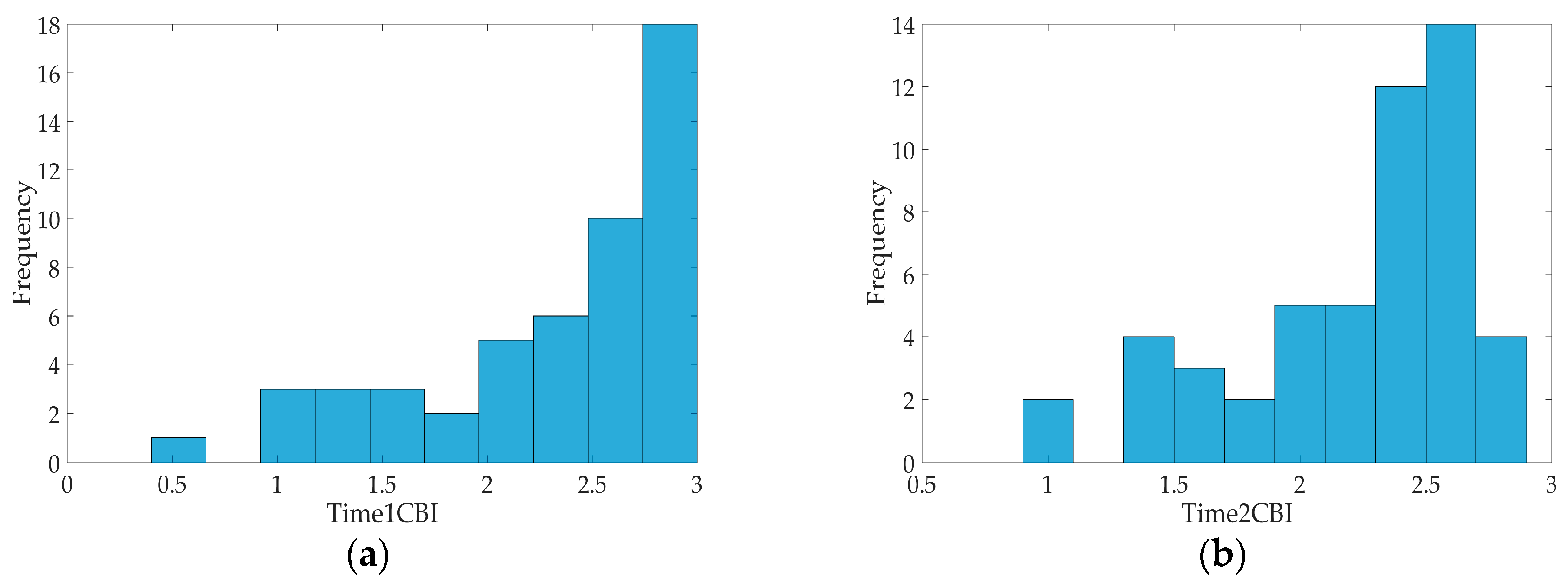
| Time1CBI | −0.8628 | 0.0109 | 0.0380 |
| Time2CBI | −0.8127 | 0.0147 | 0.0127 |
| Variable | F1 | F2 | F3 |
|---|---|---|---|
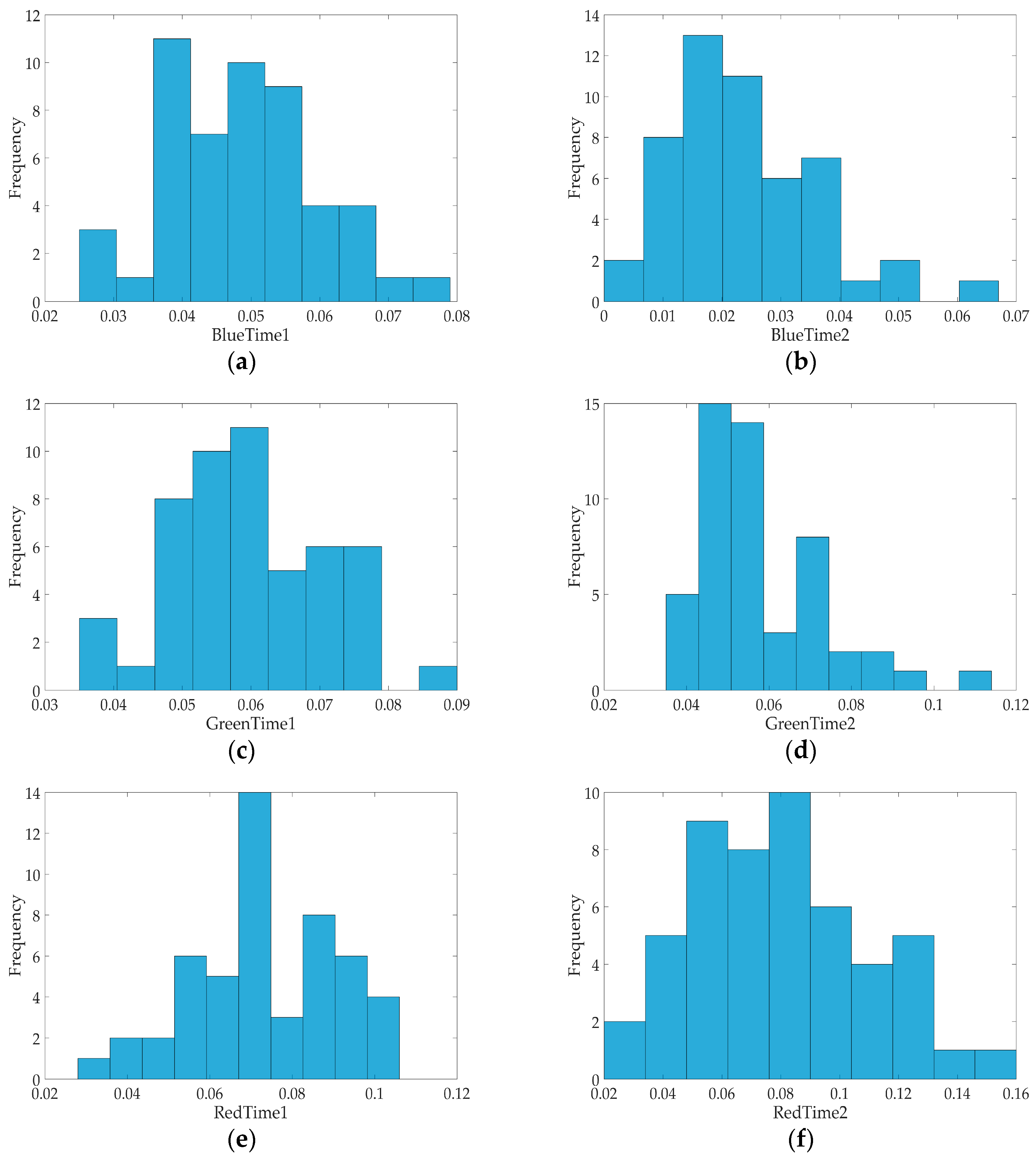
| BlueTime1 | −0.0254 | −0.0168 | 0.0269 |
| GreenTime1 | −0.0224 | −0.0270 | 0.0272 |
| RedTime1 | −0.0445 | −0.0474 | 0.0301 |
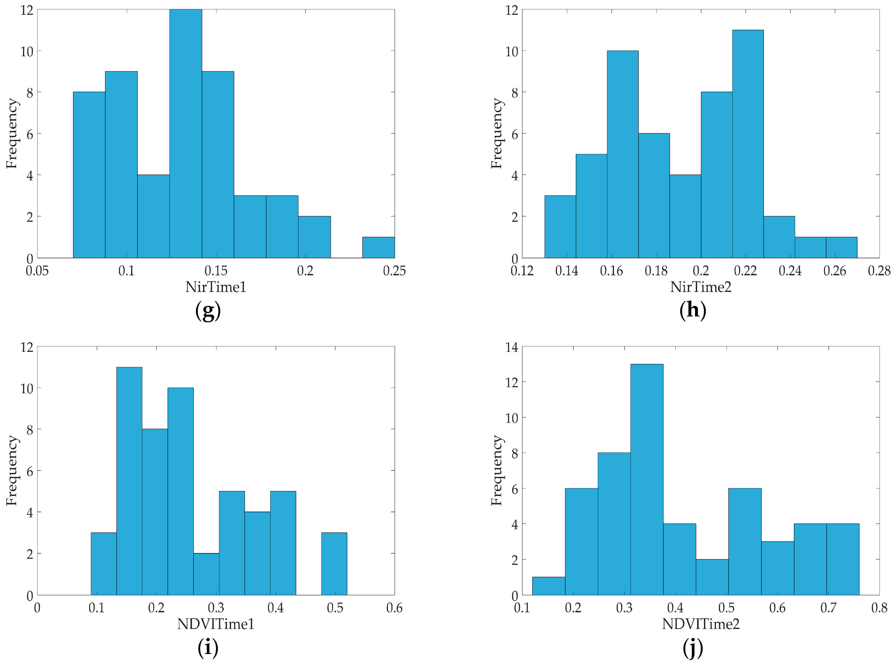
| NirTime1 | 0.0691 | −0.1078 | 0.0256 |
| BlueTime2 | −0.0495 | −0.0128 | 0.0090 |
| GreenTime2 | −0.0542 | −0.0216 | 0.0096 |
| RedTime2 | −0.1344 | −0.0360 | 0.0078 |
| NirTime2 | 0.0693 | −0.0629 | 0.0287 |
| NDVITime1 | 0.5136 | −0.0763 | −0.0722 |
| NDVITime2 | 0.8301 | 0.0497 | 0.0457 |
© 2016 by the authors; licensee MDPI, Basel, Switzerland. This article is an open access article distributed under the terms and conditions of the Creative Commons Attribution (CC-BY) license (http://creativecommons.org/licenses/by/4.0/).
Share and Cite
Dragozi, E.; Gitas, I.Z.; Bajocco, S.; Stavrakoudis, D.G. Exploring the Relationship between Burn Severity Field Data and Very High Resolution GeoEye Images: The Case of the 2011 Evros Wildfire in Greece. Remote Sens. 2016, 8, 566. https://doi.org/10.3390/rs8070566
Dragozi E, Gitas IZ, Bajocco S, Stavrakoudis DG. Exploring the Relationship between Burn Severity Field Data and Very High Resolution GeoEye Images: The Case of the 2011 Evros Wildfire in Greece. Remote Sensing. 2016; 8(7):566. https://doi.org/10.3390/rs8070566
Chicago/Turabian StyleDragozi, Eleni, Ioannis Z. Gitas, Sofia Bajocco, and Dimitris G. Stavrakoudis. 2016. "Exploring the Relationship between Burn Severity Field Data and Very High Resolution GeoEye Images: The Case of the 2011 Evros Wildfire in Greece" Remote Sensing 8, no. 7: 566. https://doi.org/10.3390/rs8070566