1. Introduction
Sugar is an important ingredient in the human diet that is mainly produced from sugarcane (
Saccharum spp. hybrid) in more than one-hundred countries within the latitude belt 37°N to 31°S [
1]. Sugarcane is also being used for bio-ethanol production, power generation from cane residues [
2], and other minor products such as bagasse, molasses and cane wax [
3]. In 2014, sugarcane crops in the world were using 27.2 million hectares [
4]. Sugarcane cultivation is widespread in Central America, covering 616,706 ha [
4], and is a key component for the Nicaraguan economy, which had 71,347 ha used for sugarcane, producing an average of 88.8 tons per ha during the harvest of 2014–2015 [
5], and 77.4% of the land devoted to sugarcane cultivation in Nicaragua is concentrated in the northwestern region of the country [
6].
Global harvest of sugarcane had a nearly sixfold increase from 1950 to 2007 while harvested area increased 3.5 times according to data collected by the Food and Agriculture Organization of the United Nations FAO [
7]. To cope with the increasing demand for sugar and other sugarcane products, many companies and farmers are expanding sugarcane plantations to new areas, clearing forest and displacing more traditional crops in tropical areas with the consequent biodiversity loss [
8,
9,
10]. Increasing yield and improving cropping efficiency are key points in a strategy for reducing agricultural expansion and environmental footprint [
11]. Proof that more attention should be given to increase yield and efficiency is that Nicaragua decreased its average yield in 7.6%, and crop areas continued to expand during harvest 2015–2016 [
12].
Sugarcane is a semi-perennial crop that tends to reach its maximum vegetative development during a grand growth stage of around 120 days to 270 days after planting in a 12-month cane [
13]. Main sugarcane varieties found in Nicaragua are from the Canal Point Sugarcane Research Station, City, Florida, US and are CP722086, CP892143 and CP731543. In general, a crop of cane takes about 12–13 months to grow in Leon and Chinandega, provinces on the pacific coast of Chinandega. Most large sugarcane plantations in Nicaragua divide their crop areas into three management zones with different planting and harvesting times. Typical harvesting periods in a year are: (i) November to January; (ii) January to March; and (iii) March to April, before rainy season starts (commonly in May) and harvesting labor increases its cost related to wet terrain and increasing transportation time of cane to the mill. In general, a cropping cycle is comprised of one plant crop and 4–5 ratoon (regrowth) crops. When ripe, the cane is usually about 2–3 m tall.
The first growth stage of sugarcane production is called the germination and establishment phase [
14]. This phase takes place at the beginning of the cycle (around 10–15 days after harvest depending on cane variety). Normally, there are areas in the plantation where stalks do not develop, either because rhizomes were damaged during previous agronomic activities such as harvest (machines passing over croplines) due to unsuccessful sprouting, or because of death of young stalks caused by pests, diseases or inappropriate water distribution [
15]. All of these causes result in the appearance of patches devoid of crop, commonly known as gaps. Farmers need to fill the gaps in the crop lines with new plants; otherwise, yield severely diminishes [
16]. According to field data, gap percentage could be as high as 30% in certain plots in Nicaragua, although this figure is subject to large uncertainty because current gap assessment methods do not obtain sufficient, precise nor cost effective information.
An operational methodology for the field assessment of gap area by measuring gap length along segments of crop lines proposed by Stolf in Brazil [
17] is being used nowadays with minor modifications. By collecting gap percentage at different plots, the manager can classify plantation zones according to crop planting quality and decide whether to replant one specific area or the whole plot. An important drawback of this method is that it requires a very intense field effort. Methods using sensors on land vehicles have been developed and tested [
18,
19] require circulating over the entire plantation, which is costly in time and fuel, and increases the risk of damaging the crop.
Agriculture has been an important field of application for Remote Sensing (RS) since the earliest days (
i.e., Neblette 1927 and 1928 in [
20]), and the interest increased with the advent of civil satellite imagery. Agricultural applications have surpassed the initial goals of crop acreage and mapping to include crop health and yield assessment. According to Atzberger [
21], there are five application domains of RS in agriculture: biomass and yield estimation, crop vigor and drought stress monitoring, assessment of crop phenological development, crop acreage and mapping, and mapping disturbance and other changes. Nowadays, precision agriculture has triggered an important effort by the Remote Sensing community to provide timely geo-referenced information on crop condition (density, vigor, phenological stage, water, nutritional status) with sufficient resolution. Crop scouting has been traditionally used to provide this information, but scouting is slow, time and labor intensive, often expensive, and the quality of its results is difficult to assess, hence the renewed interest in Remote Sensing. A wealth of research is being carried out on the use of sophisticated instruments aboard satellites and airplanes to relate critical plant properties to sensor measurements (
i.e., [
22,
23,
24]). The challenge is achieving operational methods able to be applied within reasonable budgets, a goal that has to be met at on-farm level [
20].
Abdel-Rahman and Ahmed [
25] reviewed studies on RS applications to sugarcane cultivation. Most studies were based on satellite imagery and dealt with a range of applications such as mapping sugarcane over large areas, varietal identification, detection of stress (caused by diseases, pests and nutrient and water deficiencies) and yield prediction. The authors reported many successful studies, although this was not always the case, in particular when many confounding factors were present. It is worthwhile to note that studies conducted with hand-held spectrometers (
i.e., [
26,
27]) achieved good results. Research carried out with spectrometers indicates that it is possible to retrieve nitrogen content [
28] and the nitrogen/silicon ratio [
23], which are critical data for fertilizing plans and yield forecasting. Schmidt
et al. [
29] conducted a study using a Digital Multi-Spectral Video camera mounted on a microlite, which is a small fixed-wing mono motor plane, over sugarcane fields. Results were good for the discrimination of age groups, crop moisture stress and variety identification, but not for yield prediction and fertilizer application, although the authors reported “numerous teething problems in data acquisition and camera equipment setup”.
The use of mini Unmanned Aerial Vehicles (UAV) or Remote Piloted Aircraft Systems (RPAS), a.k.a. “drones”, is revolutionizing Remote Sensing and is increasingly applied to diagnose agricultural fields [
30,
31,
32,
33]. This technology has reached operational reliability and offers the possibility to map and monitor small areas, a task that would be very expensive by an aircraft, especially when the farm to monitor is not close to an airport. Therefore, RS from UAVs can be, in principle, a solution to incorporate RS at on-farm level. Nevertheless, it also must be considered that sensors aboard mini UAVs must be miniaturized versions of those traditionally used from satellites and airplanes because size and weight constraints, with the resulting lower quality, which has to be added to the inherent instability of a small platform. Therefore, it is important to test whether a particular agricultural application can be satisfactorily achieved by using instruments aboard a mini UAV.
Considering the critical importance of a correct assessment and the mapping of gap percent for optimizing sugarcane cultivation, the goal of this study was to assess, within the economic constraints of a developing country, the appropriateness of conventional digital imagery acquired from a mini-UAV for this purpose, using a photo-interpreted version of Stolf’s methodology as a reference.
2. Methods
2.1. Study Site and Aerial Campaign
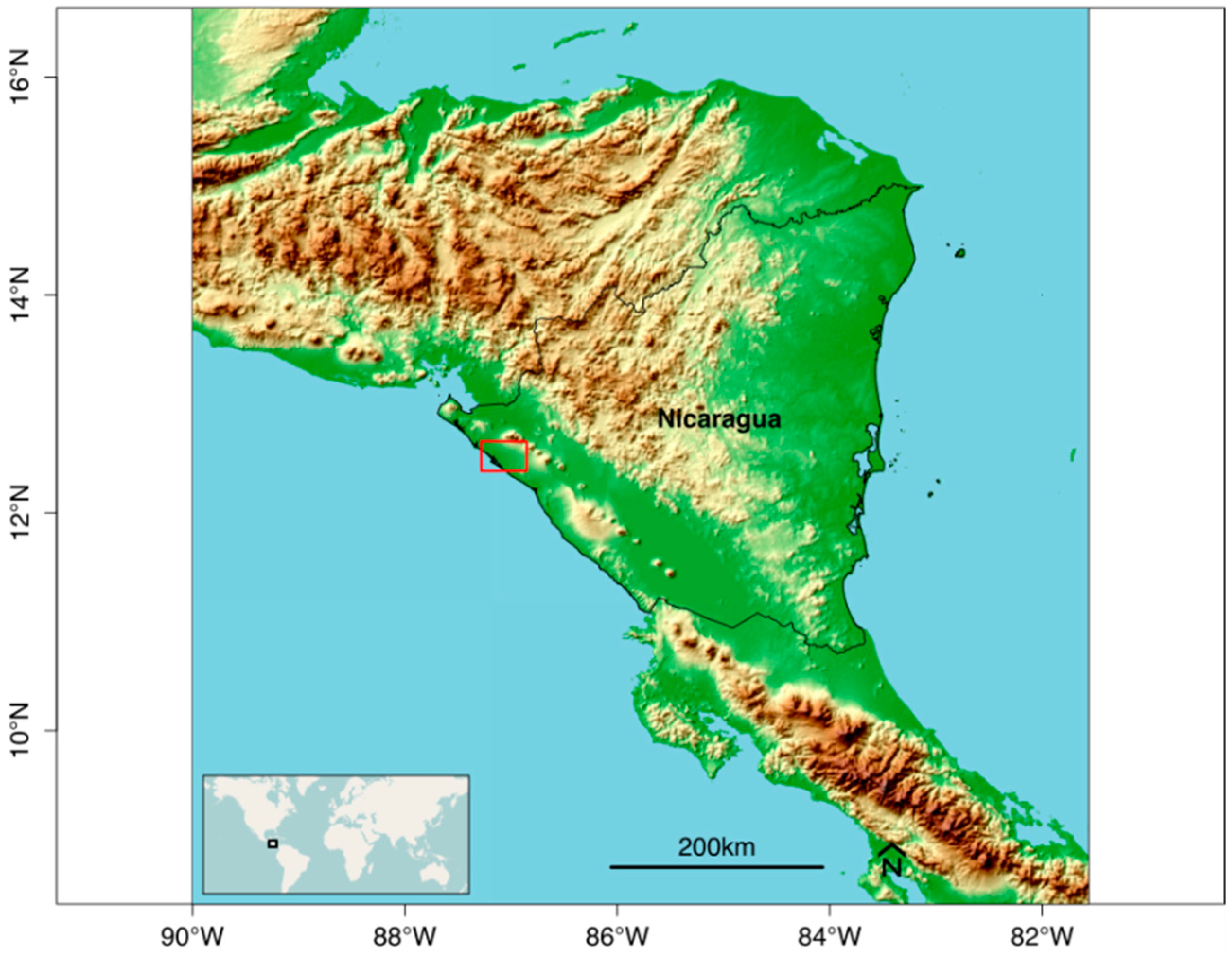
The UAV imagery was acquired over a plot of sugarcane named El Gobierno (12.448192°N, 87.053016°W and 19 m above sea level). The El Gobierno plot belongs to a 12,000 ha plantation located in the NW of Nicaragua, Central America (
Figure 1) in the departments of Leon and Chinandega. The region has tropical savanna climate classified as “Aw” in the Köppen and Geiger system. Daily mean temperature ranges from 27.0 to 27.4 °C and rainfall from 1592 to 1979 mm. [
34]. Most common soil orders in the area are inceptisols, entisols and vertisols, which are of volcanic origin [
35].
The flight mission was planned with Lentsika software (2010 version from CEPED co, Torino, Italy), which transformed the overlaps and pixel size requirements into flight commands and parameter information for the autopilot. However, Lentsika software does not take into account specific camera features that are required to accomplish an accurate pixel size estimation; thus, further calculations had to be made and the Lentsika information was used only as a rough estimation.
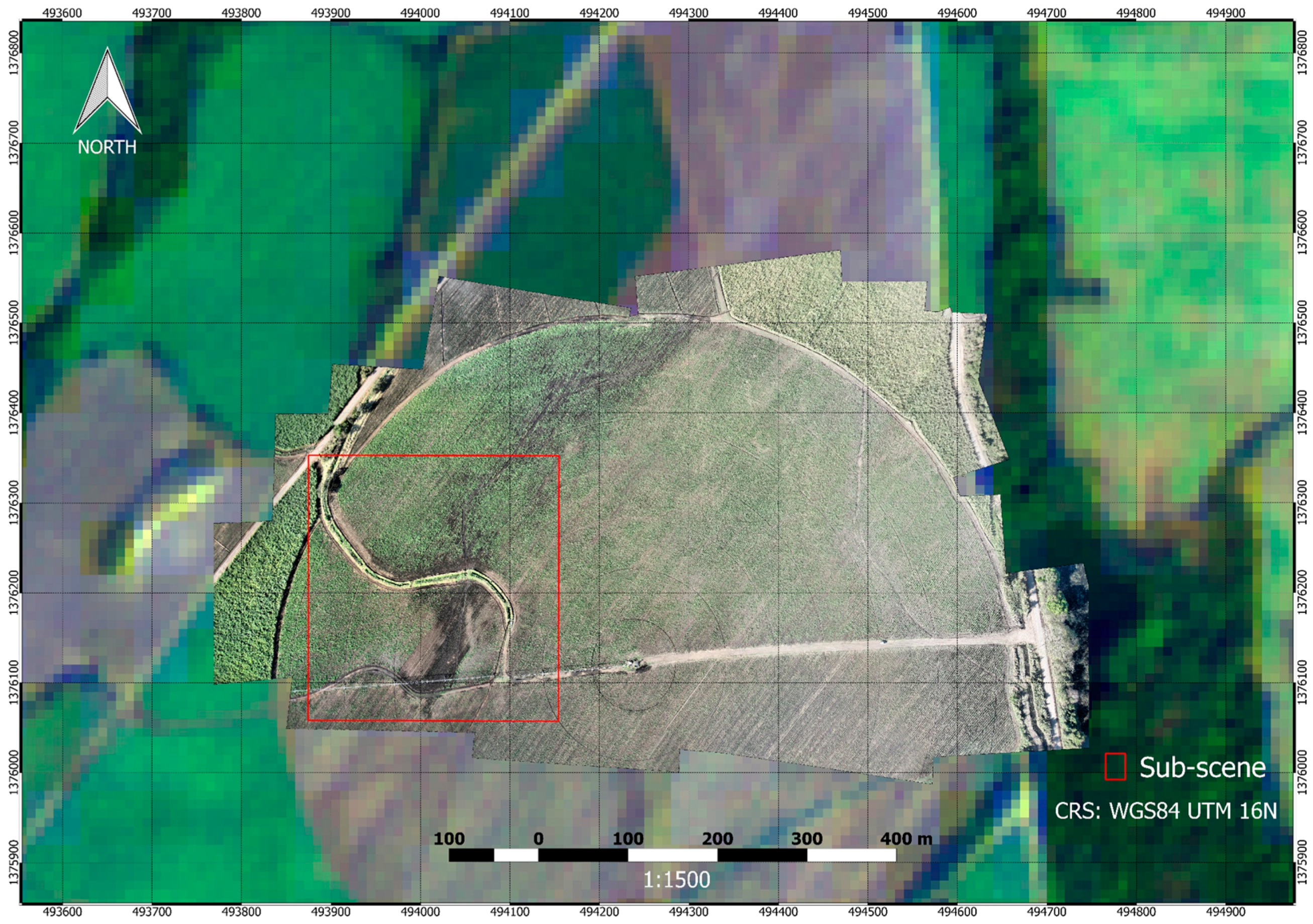
A 16 min flight at 190 m above ground level with an overlap of 90% and a sidelap of 50% was carried out with the UAV to cover 24 hectares of the El Gobierno plot, registering 134 images with an average pixel resolution of 4.7 cm (
Figure 2).
2.2. UAV System
A Cropcam UAV with HORIZON ground control software (Micropilot Co., Stony Mountain, MB, Canada) was used for aerial image acquisition. The Cropcam weighs 3 kg, has a wingspan of 1.8 m and a maximum endurance of 45 min. In practice, due to payload weight, wind speed and airframe modifications for a more stable flight and safe landing, endurance is reduced to 20 min at an average speed of 60 km/h. Our system includes a military grade autopilot unit (MP2028), which is a electromechanical system used to guide the plane without human assistance, in a radio controlled glider airframe. The autopilot guides the plane using GPS technology and differences in air pressure with a pitot tube in order to improve the speed control, flight performance and stability. The system has telemetry capacities, and transmits its position (x, y, z) to a computer using a radio modem, allowing the user to control the plane either via the radio control transmitter or via the computer. The autopilot supports multiple features and is programmable to fly a route and trigger a camera or other payload at specific locations.
The UAV was equipped with a conventional consumer grade still camera, a Canon SD780is with 5.9 mm focal length and a 1/2.3″ CCD sensor (6.17 mm × 4.55 mm) of 12.1 mega pixels, that was mounted under the wing (Canon Inc., Tokyo, Japan).
2.3. Image Mosaicking and Geo-Referencing
A Mosaic with pixel resolution of 4.7 cm was produced by stitching the 134 images through PTGUI software, version 8.3.10 (New House Internet Services BV, Rotterdam, The Netherlands), and geo-referenced using the Georeferencer Tool plugin of Quantum Geograpic Information System (QGIS) software, version 1.7.4 [
36] with a first-degree polynomial transformation. A high accuracy GPS for ground references was not available; therefore, pairs of ground control points were identified on the mosaic and Google Earth imagery that was used as a reference. The simple first-degree polynomial transformation could be used because the terrain was flat, the area small (24 ha) and few pairs of ground control points could be reliably identified. The resultant mosaic had a geometric error of 2.04 m estimated by identifying additional pairs of corresponding sites on the mosaic and Google Earth imagery. Reasons for this geometric error are given in discussion.
2.4. Stolf Method
Stolf [
17] developed a methodology for assessing crop planting quality in sugarcane plantations based on gap evaluation, in which the lengths of gap segments are measured and added up along crop lines in the field. For practical reasons, gap segments are defined as those segments with no sugarcane plants or decayed sugarcane plants longer than 0.5 m. The method is applied by deploying a measuring tape on the ground and using a 0.5 m stick as the reference of minimum gap length. The length of so-defined gap segments is accumulated and the percentage of gap in a given distance is reported. Planting quality levels are defined based on gap percentage intervals as reproduced in
Table 1.
Obviously, not all crop lines can be measured at their entire length, as this would imply measuring (and walking) 6.5 km along crop lines for just a 1 ha plot. Aware of this, Stolf proposed measuring 4–5 random samples of 20–25 m for a 7 ha plot. Actually, current practices in El Gobierno are more intense: 1 random sample of 30 m is measured for each 0.7 ha plot (locally known as “manzana”).
2.5. Processing
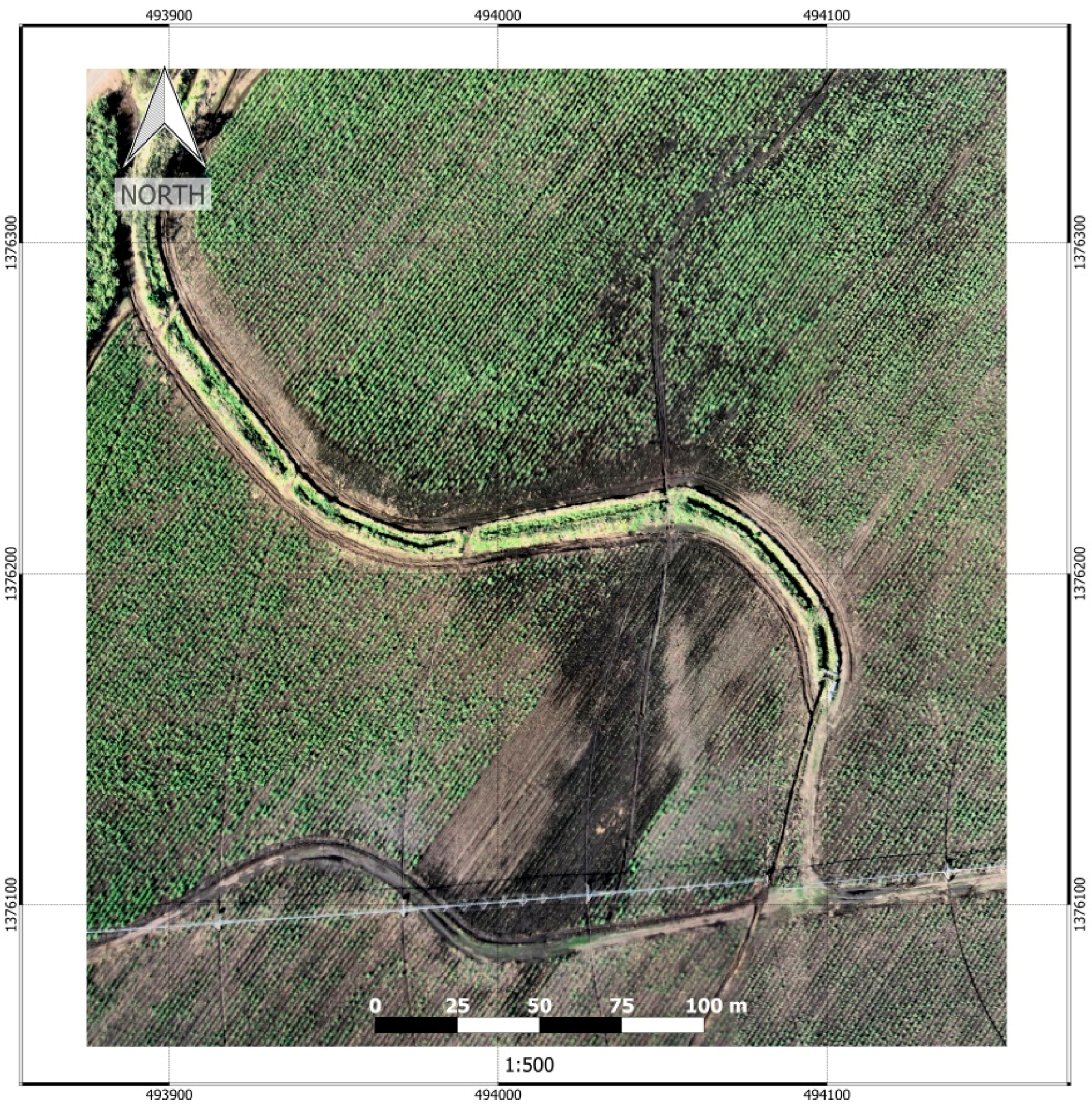
For this pilot study, we selected a sub-scene of 6272 lines × 5941 columns (8.2 ha) in the SW corner of the mosaic (
Figure 3) and calculated a coarsened version with 23.5 cm resolution (1254 lines × 1188 columns) that was used for processing, keeping the higher-resolution version (4.7 cm per pixel) for photo-interpretation. As we detail in the following sub-sections, the processing method had two parts. First, we applied a supervised classification to create a binary image coded as “sugarcane” and “gap”, where “gap” included bare soil and decayed plant material. Second, we estimated Gap percentage for a grid of 10 m × 10 m cells, and Crop Planting Quality Level following Stolf’s standard thresholds (
Table 1). This second step involved estimating Linear Gap percentage (gap estimates along lines) from the Gap percent based on the classification (thus a 2D estimate). Both processing steps required reference information that we produced through photo-interpretation of the 4.7 cm resolution mosaic.
All statistical processing and graphics were performed in R [
37], with packages rgdal [
38], raster [
39], rgeos [
40], MASS [
41], ggplot2 [
42] and plyr [
43]. Display and exploration of imagery and spatial data sets was done in QGIS [
36].
2.5.1. Reference Information
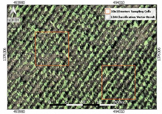
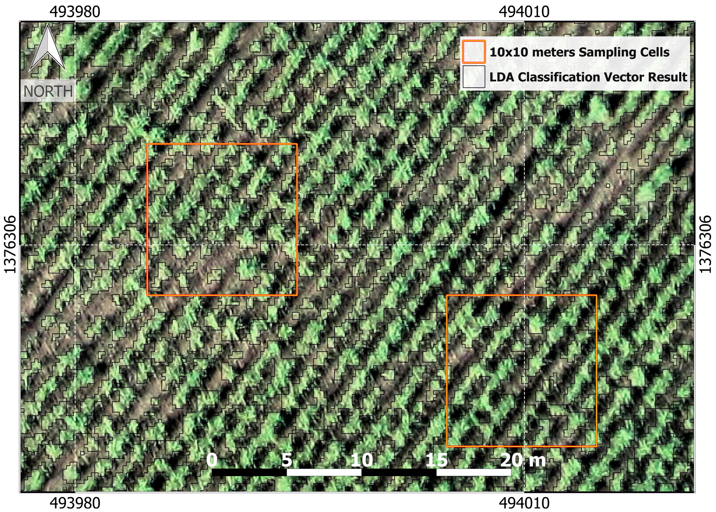
Actual field information was not available for this study, so we created two data sets of reference information (acting as “ground truth”) through interactive photo-interpretation of the image at 4.7 cm resolution, in which plants could be distinguished. For the classification, we generated training and validation sets of point sites for which we determined whether the corresponding cover was sugarcane or gap. We defined a regular grid of 31 × 28 (768) cells of 10 m of side and selected a random subset of 25 cells. In order to create a training set of site observations for the supervised classification, we selected a random set of 300 point sites within the selected cells. These 300 points were complemented by a set of 10 point sites randomly distributed over an area almost totally devoid of sugarcane and with notoriously darker soil. Photo-interpretation diagnosed each point site as “fresh sugarcane”, “regular soil or withered sugarcane” or “dark soil”. We discarded one point site because of dubious interpretation.
For the estimation of Linear Gap percentage, we digitized crop lines and gap lines in the random subset of 25 grid cells. This procedure actually mimics Stolf’s method as performed in the field (see
Section 2.4), although with much higher sampling intensity. We wrote an R script to import the shape files and calculated total row length, total gap length, Linear Gap Percentage and Crop Planting Quality Levels for each random cell.
In order to define the potential crop area, we digitized polygons of constant width (0.8 m) with axes coincident with those of the crop rows. We used these polygons to define the crop mask. We also digitized a mask of roads that included a small and narrow area (0.1 ha) between the limit of the road and the NW edge of the area of study to define areas not to be included in the surface calculations.
2.5.2. Classification
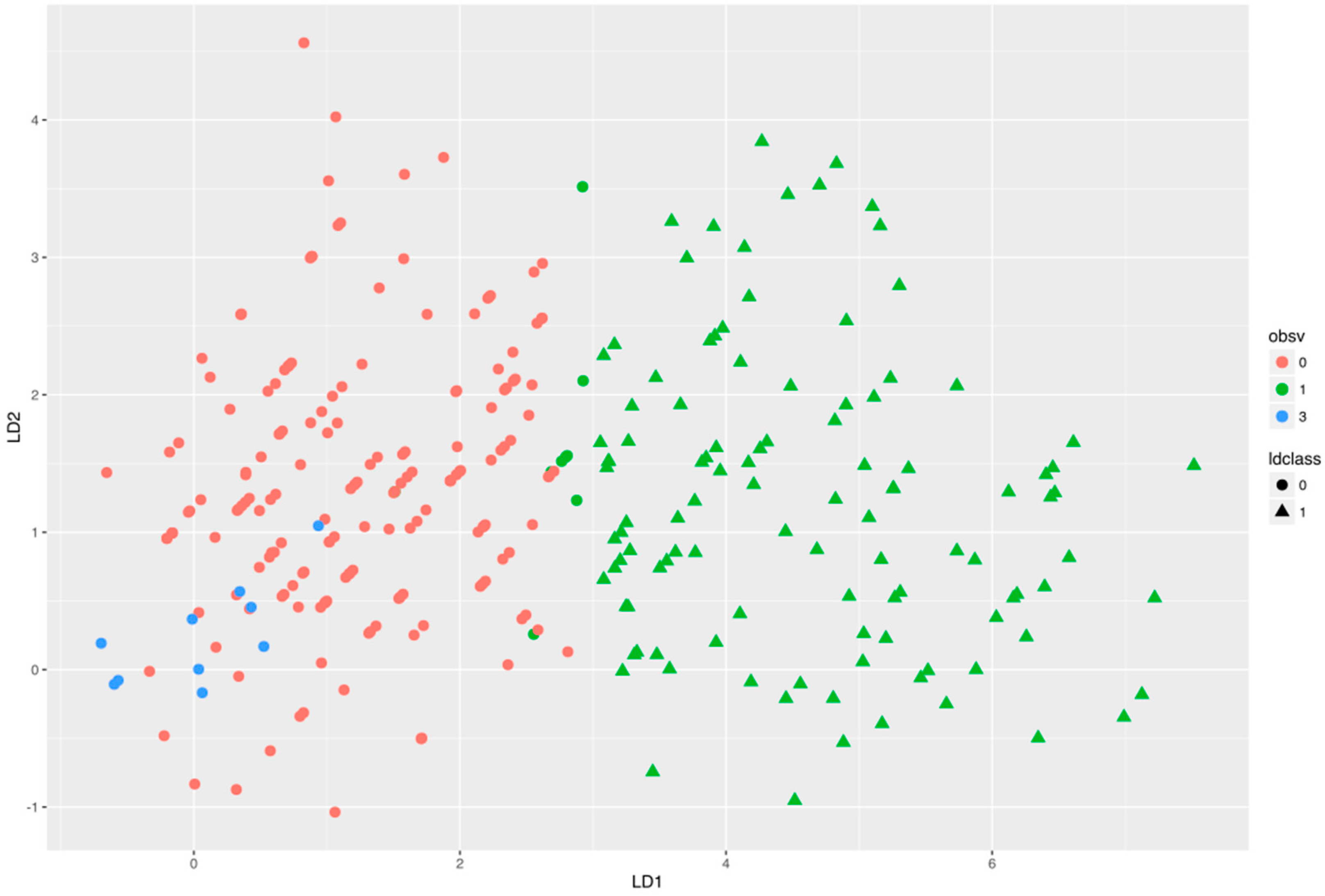
We retrieved the red (R), green (G) and blue (B) values corresponding to the 309 point sites from the image and generated a training data set with the red-green-blue bands (RGB) values as variables, and the diagnosed classes as grouping factors for running a Linear Discriminant Analysis (LDA [
44]). LDA produced the transformation matrix for the canonical components and a cross-validated classification of the point sites. Cross-validation is a built-in method in the LDA function in R that consists of iteratively calculating the LDA excluding one element from the data set and predicting the class of the excluded element. This way, all elements were classified by a model that excluded the element for the fit. LDA output was used to display the point sites data on the canonical space, to build the confusion matrix and to calculate overall producer and user accuracies [
45]. Finally, we used the fitted LDA model to predict the class of all pixels in the image, resulting in the “Classified Raster Layer”.
2.5.3. Linear Gap Percentage and Crop Planting Quality Maps
We calculated “Gap Percentage” for each grid cell as the percentage of gap pixels in the corresponding areas of the Classified Raster Layer and within the area defined by the crop mask, excluding the area defined by the roads mask.
For the random sub-sample of 25 grid cells for which we had previously estimated “Linear Gap Percentage” by digitizing on the 4.7 cm resolution image (see
Section 2.5.1):
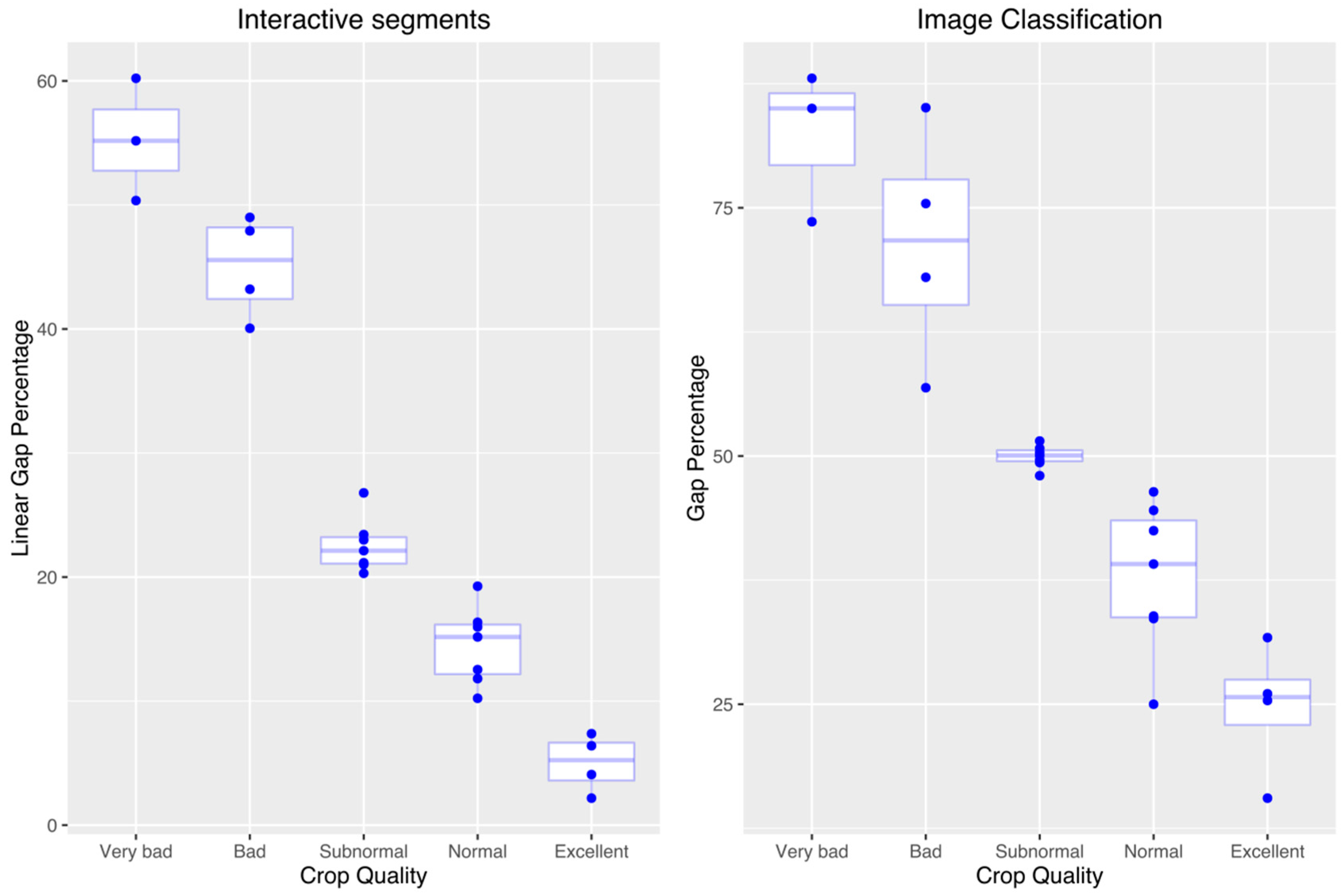
- (i)
We compared boxplots of Gap and Linear Gap Percentage by “Crop Planting Quality Levels”, to visually explore the appropriateness of the image-derived information to define “Crop Planting Quality Levels”.
- (ii)
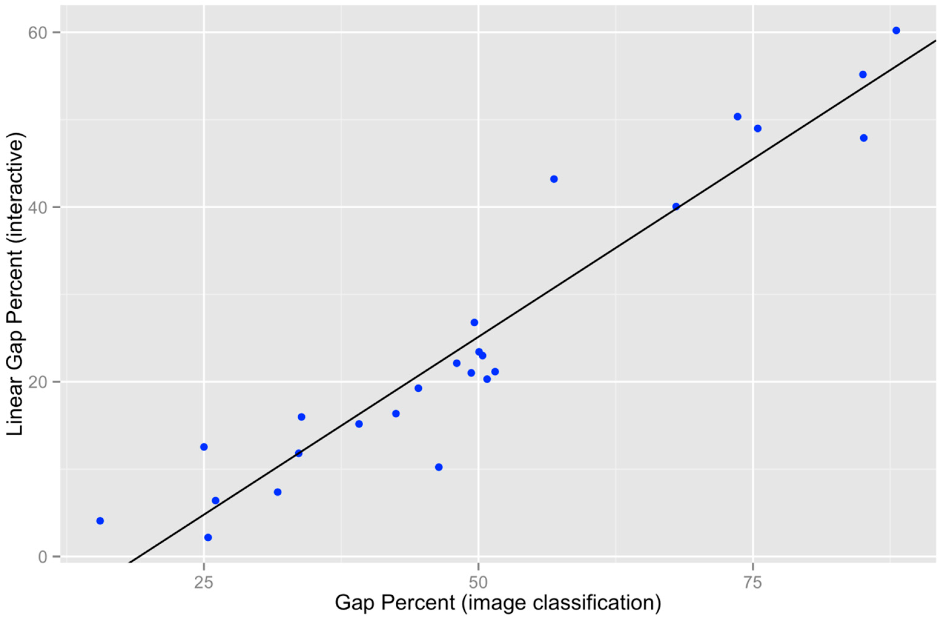
We fitted a linear regression model of “Linear Gap percentage” vs. “Gap percentage”.
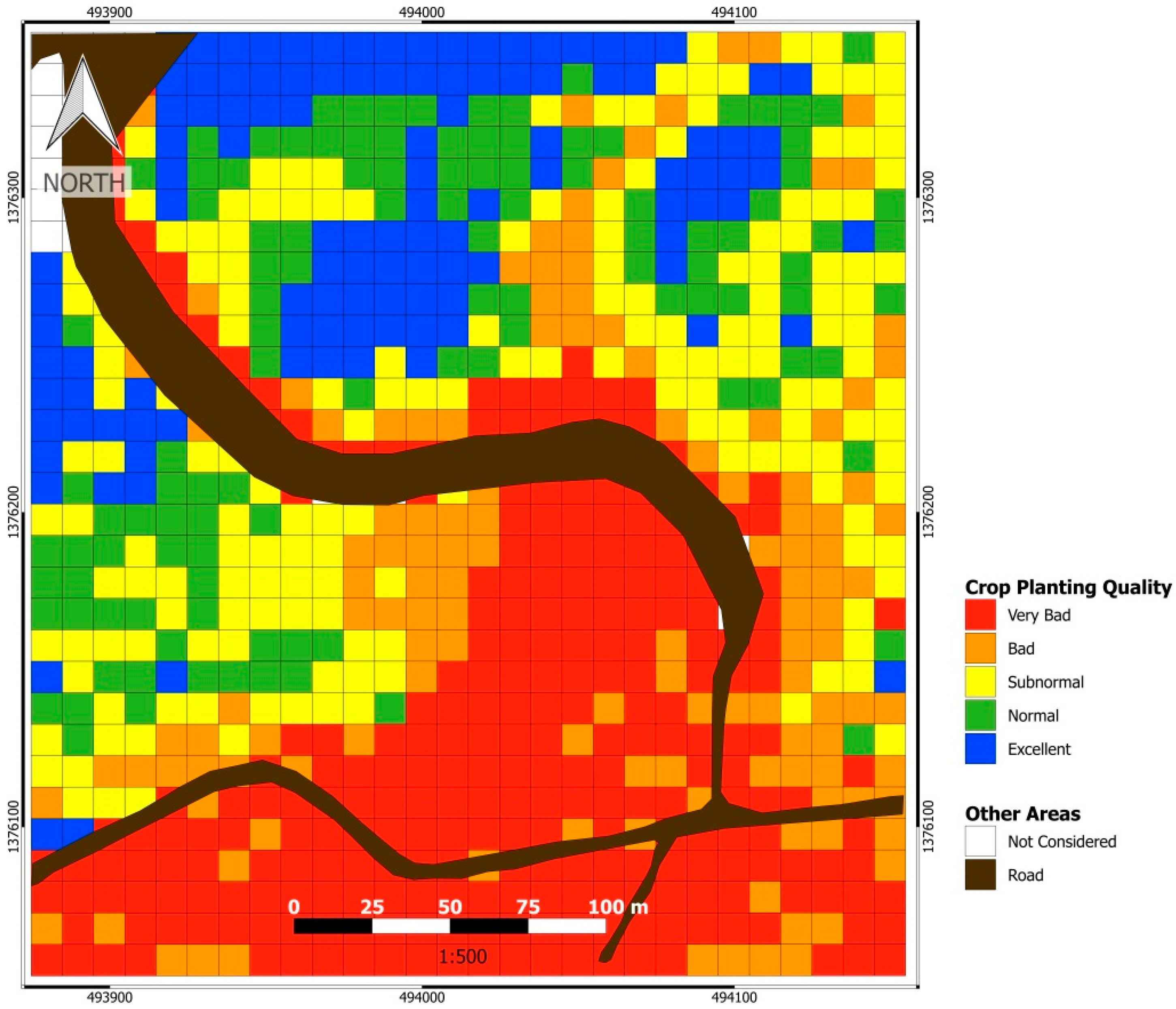
We applied the regression coefficients to calculate predicted “Linear Gap percentage” values to all grid cells and, from them, predicted “Crop Quality levels” by applying Stolf’s standard thresholds (
Table 1).
The accuracy of the regression model was assessed by its coefficient of determination (R2) and root mean square error (RMSE), while the accuracy of predicted and the observed “Crop Planting Quality levels” was assessed by cross validation. To this end, we wrote an R script in which the regression is calculated with all data (from the subset of grid cells) but one, and the threshold applied to determine the predicted “Crop Planting Quality Level” of the excluded element. The script iterates in a manner that each element is excluded from the calculation of the regression model used to determine its predicted “Crop Planting Quality Level”. These observed and predicted values were collected in a confusion matrix, thus allowing for an independent estimate of the accuracy, which was measured by the Spearman correlation coefficient (as corresponds to interval variables).
4. Discussion
Our methodology is operational and outperforms current field methods, as the classification error is small and clearly compensated by the superior spatial intensity of an image-based method: current practices of field gap evaluation in El Gobierno (one segment of 30 m evaluated every 0.7 ha) would have implied evaluating 11 segments of 30 m, a length approximately equivalent to that of all crop lines within five plots of 10 m × 10 m, that is only about 0.45% of the total crop lines length. While this sampling intensity, which requires a very significant human effort, might provide some insight for monitoring overall crop planting quality, it is clearly insufficient to map gap percentage and derived crop planting quality, which makes re-planting activities very difficult to guide. Instead, our method uniformly maps Crop Planting Quality for the whole area by units of 10 m × 10 m.
In practice, for applying this methodology on a regular basis to a given plantation, Stolf’s thresholds for Crop Planting Quality Levels would be calculated in terms of the classification-based gap percentage at the beginning of the study: the regression model relating linear (interactive) and classification-derived Gap percentages would be fitted once and would hold as long as the geometric arrangement of the plantation (and thus the fit of the rectangular mask to the crop rows) remain the same.
According to our evaluation, there is a very good agreement between our estimate of Crop Planting Quality and the one resulting from Stolf’s method. The observed small discrepancy is due to classification error and to the differences in Gap percentage estimates between the linear (interactive) and the classification-based methods. Future improvements to the method should thus concern these two aspects, with the addition of improving geometric accuracy. We briefly review these possible improvements in the rest of the Discussion and point out possible future related studies.
Besides the obvious improvement of using a better camera, improved image processing methods could reduce classification error further. Object-based recognition [
46,
47] could improve identifying sugarcane plants [
48], and more sophisticated classification methods (notably Support Vector Machines [
49,
50]) will probably outperform LDA. It can be argued that requiring a training set of diagnosed sites could be seen as a drawback. While testing completely unsupervised methods is certainly of interest, generating a training set is not a very time-consuming task and the detailed inspection of the imagery is always interesting and worthwhile. The classification approach that is crucial in this methodology assumes that color is uniformly registered across the mosaic, which implies that care must be taken at image acquisition and mosaicking. While methods such as Contrast Limited Adaptive Histogram Equalization (CLAHE [
51]) can be used in those cases in which the mosaic is not uniform, angular effects deserve more careful consideration in future studies [
52].
Part of the dispersion of the regression model relating linear (interactive) and classification-derived Gap percentages is caused by the rectangular masks of the crop rows not fitting the actual irregular limits of the rows equally everywhere, as mentioned in
Section 3.2. Image segmentation could be used to delineate crop rows [
53] and produce an image-derived irregular mask fitting the actual crop instead of the digitized regular rectangles. Image segmentation has been applied to Unmanned Aerial System (UAS)imagery with similar purposes in orchards and vineyards (
i.e., [
54,
55]) In our case, the consistent generation of an adaptive mask would greatly increase the stability of the relationship between the linear (interactive) and the classification-based estimates of Gap percentage.
The elementary mosaicking and georeferencing methods that we have applied in this study are acceptable for very flat surfaces and yet have resulted in a large geometric error compared to pixel resolution. This error can be tolerated in this application because the final Crop Planting Quality product is a 10 m × 10 m grid, but would be an obvious problem for final products demanding finer resolution. More sophisticated mosaicking methods performing ortho-rectification are required in general for UAS imagery. Several commercial alternatives exist that use structure from Motion (SfM [
56,
57]) based software that apply automatic tie point generation, bundle block adjustment technology and efficiently generate ortho-rectified mosaics and digital surface models (also known as crop surface models, CSMs) with homogeneous radiometric responses. However, these types of products require ground control points (GCP) with high geometric accuracy, which is not easy for areas without unclassified high-resolution official orthophotomaps as in this case. Deploying markers on the ground and reading their coordinates with sub-metric (or even centimetric) accuracy is a very effective solution. Unfortunately, sub-metric or centimetric GPS equipment was not available for this study, but it is clearly a very needed piece of equipment for future campaigns, and acquisition should be facilitated by the current trend towards low-cost real time kinematics GPS (orRTK GPS) systems. Nevertheless, it must be noted that, while deploying ground markers on small areas such as the one of the sub-scene processed in this study (8.2 ha) is feasible, deployment of markers on larger areas such as the one of the entire mosaic (24 ha) will require a significant effort. This situation is pushing towards alternatives such as using RTK GPS during flight to get highly accurate camera locations data, thus avoiding the need of setting physical ground reference at the site while still getting high accuracy in final mosaic products [
58].
Extending the method presented in this study to large plantations would have a considerable interest, making relevant the fact that Remote Sensing from UAVs should not be considered outside the framework of Remote Sensing from other vehicles. Large plantations will require optimizing pixel size to cover a large extent while keeping computing requirements within feasible limits on one hand, and sufficient gap detection on the other. Such an optimization implies a sensitivity analysis of gap detection to pixel length for each considered instrument (
i.e., [
59,
60,
61]), a task for which the integration of UAV Remote Sensing from a range of heights, and satellite (
i.e., Sentinel-2) imagery would be most useful.
We have used Stolf’s method in this study to demonstrate that image-derived gap percentage can map Crop Planting Quality levels as an effective and spatially intense alternative to field-estimated linear gap percentage because Stolf’s method is currently the most common method. In addition, gaps are readily assessed by photo-interpretation of very high-resolution imagery because of their high contrast to fresh sugarcane. Nevertheless, estimating Crop Planting Quality based on gap percentage is not necessarily the only or the best method. It might very well be the case that our estimate of gap percentage could be better related to a more formal measure of crop quality such as green biomass rather than linear gap percent. In other words, alternative measures of crop planting quality at sampling sites in the field could be both more relevant agronomically and better related to image-derived information. Crop surface models, which would require high accuracy GCP and stereo images, should be investigated in sugarcane as it has provided useful data to study biomass in rice [
62] and estimate yield in corn in conjunction with spectral data [
63]. Furthermore, as multi-spectral imagery can provide information beyond gap percentage, for example on plant condition (see Introduction section), using a multi-spectral camera with bands going into the near-infrared region of the electromagnetic spectrum would represent an important improvement. It is relevant to note, though, that addressing the issue of remote sensing of plant condition goes well beyond simply using a better sensor, but involves ground sampling procedures and appropriate analytical methods because photo-interpretation methods (as those used here) cannot provide reliable information on quantitative plant properties. In addition, image processing and information retrieval methods would have to suit leaf size constraints, including finer pixel size and object-based analysis (
i.e., [
64]).
5. Conclusions
Current practices of field gap evaluation in sugarcane plantations are highly demanding in terms of human labor and hence of very limited spatial intensity. For example, in this area of study, the rate was one segment of 30 m evaluated every 0.7 ha, which implies a length approximately equivalent to 0.45% of the total crop lines length. This sampling intensity is clearly insufficient to map gap percent and derived crop quality, which makes re-planting difficult to guide. Instead, our method, based on the processing of the digital mosaic of UAV images, estimates linear gap percentage with an RMSE of only 5.04 for a grid of 10 m × 10 m resolution, and derived Crop Planting Quality highly agreed with those derived from a photo-interpreted version of the currently used Stolf’s method (Spearman’s correlation coefficient 0.92). Furthermore, a map of canopy gaps is produced with high overall accuracy (97% estimated by cross-validation; 92.9% estimated by independent sample) at 23.5 cm resolution. Although some image processing improvements in image quality and processing can probably further reduce the error, the current methodology is ready for immediate operational application.
Previous results based on satellite imagery and hand-held spectroradiometry, together with the effectiveness of UAVs to image sugarcane crops at high resolution and the power of current processing methods as shown in this article, indicate the interest of replacing the conventional RGB imagery used in this study with multi-spectral imagery, to go beyond gap mapping into mapping plant status.


