Article

Abiotic Controls on Macroscale Variations of Humid Tropical Forest Height

1
Institute of the Environment and Sustainability, University of California, Los Angeles, CA 90095, USA
2
Earth and Environment, Boston University, Boston, MA 02215, USA
3
Jet Propulsion Laboratory, California Institute of Technology, Pasadena, CA 91109, USA
4
Natural Resource Ecology Laboratory, Colorado State University, Fort Collins, CO 80523, USA
5
Agence National des Parks Nationaux, Battery 4, Libreville B.P. 20379, Gabon
*
Author to whom correspondence should be addressed.
Remote Sens. 2016, 8(6), 494; https://doi.org/10.3390/rs8060494
Submission received: 31 March 2016 / Revised: 29 May 2016 / Accepted: 7 June 2016 / Published: 14 June 2016
(This article belongs to the Special Issue Remote Sensing of Vegetation Structure and Dynamics)

Abstract

:
Spatial variation of tropical forest tree height is a key indicator of ecological processes associated with forest growth and carbon dynamics. Here we examine the macroscale variations of tree height of humid tropical forests across three continents and quantify the climate and edaphic controls on these variations. Forest tree heights are systematically sampled across global humid tropical forests with more than 2.5 million measurements from Geoscience Laser Altimeter System (GLAS) satellite observations (2004–2008). We used top canopy height (TCH) of GLAS footprints to grid the statistical mean and variance and the 90 percentile height of samples at 0.5 degrees to capture the regional variability of average and large trees globally. We used the spatial regression method (spatial eigenvector mapping-SEVM) to evaluate the contributions of climate, soil and topography in explaining and predicting the regional variations of forest height. Statistical models suggest that climate, soil, topography, and spatial contextual information together can explain more than 60% of the observed forest height variation, while climate and soil jointly explain 30% of the height variations. Soil basics, including physical compositions such as clay and sand contents, chemical properties such as PH values and cation-exchange capacity, as well as biological variables such as the depth of organic matter, all present independent but statistically significant relationships to forest height across three continents. We found significant relations between the precipitation and tree height with shorter trees on the average in areas of higher annual water stress, and large trees occurring in areas with low stress and higher annual precipitation but with significant differences across the continents. Our results confirm other landscape and regional studies by showing that soil fertility, topography and climate may jointly control a significant variation of forest height and influencing patterns of aboveground biomass stocks and dynamics. Other factors such as biotic and disturbance regimes, not included in this study, may have less influence on regional variations but strongly mediate landscape and small-scale forest structure and dynamics.

Graphical Abstract

1. Introduction

Humid tropical forests play an important role in the global carbon cycle by covering only 7%–10% of the Earth land surface, yet they contain about 40%–50% of the terrestrial carbon stock [1], and are responsible for about 70% of terrestrial carbon sink [2]. With increasing amount of high-resolution remote sensing data and availability of networks of ground plots, understanding the fine scale variations of forest structure and dynamics and their biotic and abiotic controls have improved significantly over the past decade [3,4,5,6,7,8]. However, understanding macroscale variations of forest structure and their ecological and environmental controls lags behind. This is because existing ground plots are sparsely distributed and not suitable for macroscale studies [9,10], and investments in design and implementation of regional scale ecological studies are inadequate.
The heterogeneity of the forest structure in humid tropics may come from: (1) small-scale dynamics such as tree falls, mortality, and recruitment [11]; (2) large scale disturbance in the form of storms and droughts [4,7,12,13]; (3) natural environmental variations in climate, soil, and geology [14,15,16,17]; and (4) evolutionary processes forming the phylogenetic variations and the biogeography of forest species [18,19]. In addition, recent or past human induced land use activities such as small and large-scale forest clearing or tree extractions may have also influenced the variations of forest structure. This heterogeneity, generally using tree height and/or diameter as a measurable quantity, is therefore a reflection of environmental impacts on the local vegetated surface in humid tropical forests [20].
At continental scales, individual-based ground measurements suggest large regional differences in canopy height with tallest trees reported in tropical Asia, followed by forests in Africa and America [21]. These patterns, however, may not directly translate to variations of forest above ground biomass (AGB) as diameter and wood density of trees also control the forest AGB and influence the landscape heterogeneity [22,23]. Over sharp gradients such as tropical montane forests, tree height decreases with the rising elevation as proxy for decreasing temperature [24], present a combined effect of both climatic factors and edaphic properties. Studies using field observations also show that the aboveground live biomass variations at landscape scales, which are highly related to the variation of large trees [25], are positively correlated with soil texture gradients and topography. In addition to the impact of soil structural properties, nutrient availability in soil, such as exchangeable cations, carbon, nitrogen, and pH, as well as soil phosphorus status, have been found to have a non-negligible impact on the tropical forest height structure and its dynamics [17]. Therefore, height of trees may be considered a key functional trait at each location in tropical forests, capturing both the phylogentic variability of species, differences in allometry, and their growth trajectory [26].
To understand and quantify the variability and the controls on forest mean and maximum tree height in tropical forests, a systematic observation of tree height is required. Existing ground observations documented in research networks of plots have contributed significantly in understanding the local characteristics of forest structure [3,21]. However, the plot networks are not designed to provide enough samples on regional or continental scale variations. Alternatively, remote sensing techniques can provide systematic observations of tropical forest structure using recently advance active sensors such as lidar (Light Detection and Ranging) and radar (Radio Detection and Ranging) from airborne and spaceborne platforms [27,28,29].
Here, we focus on investigating the natural environmental controls on macroscale variations of tropical forest heights. Our study will include only humid tropical forests including low land and high land terra firme and swamp forests across elevation, soil, and climate gradients. We exclude dry and woodland forests in tropical regions due to their readily distinct distributions in different climate and soil conditions (REF). We use observations from the Geoscience Laser Altimeter System (GLAS) satellite between 2004 and 2008, measuring forest top canopy height (TCH) and vertical profile at about 0.25 ha effective footprint size across humid tropical forests. We perform statistical analysis of the variations of forest canopy height at regional scale, linking variations of top canopy tree height to the environmental controls. We also identify individual climate and edaphic factors that significantly contribute to the TCH variation by accounting for the spatial autocorrelation effects. As an independent systematic sampling of forest vertical structure, the GLAS-derived TCH data give us the opportunity to study the relationships between humid pantropical forests and the associated environmental influences with statistically large samples covering the entire tropical region.

2. Materials and Methods

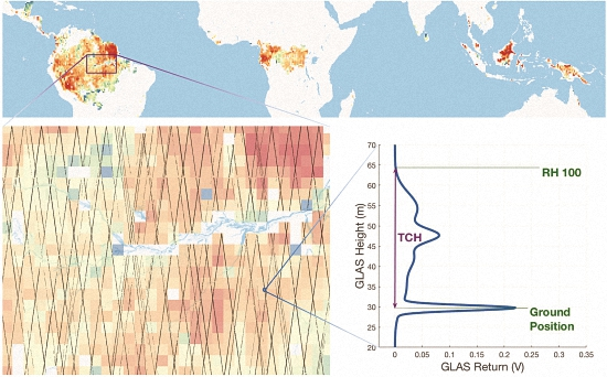
2.1. Remote Sensing Data

We used three remote sensing-based data sets in our study. First, the land cover (LC) map from Globcover 2009 [30] was used to define our study region (57°S–30°N) and pick dense tropical forest pixels only. We selected classes 40 (Closed to open (>15%) broadleaved evergreen and/or semi-deciduous forest (>5 m)) and 160 (Closed (>40%) broadleaved forest regularly flooded-Fresh water from the Globcover map and defined them as tropical dense forests). All other pixels were marked as invalid and not included in further calculations. Although the area of flooded forests is underestimated in Globcover due to the lack of SWIR band in the MERIS sensor [31] and significant confusion in classification because of the similarity of the spectral reflectances, by combining the two classes, we circumvent possible errors of mis-classification and use the overall domain of humid tropical for this study.
For forest structure, we rely solely on the measurements from GLAS lidar data because of the extensive systematic coverage over tropical forests for a period of more than four years (2003–2008). GLAS sensor aboard the Ice, Cloud and land Elevation Satellite (ICESat) is the first spaceborne waveform sampling lidar instrument for continuous global observation of the Earth. It emits short duration laser pulses and records the echoes reflected from the Earth’s surface [31]. When the surface is vegetated, the return echoes or waveforms are the function of the canopy vertical distribution and ground elevation within the area illuminated by the laser (the footprint), thus reflecting the canopy structure information [1,32,33]. From each GLAS lidar footprint, we selected the top canopy height of the lidar waveform, representing the maximum height of trees of the forest sampled within the lidar footprint. Top canopy height (TCH) is calculated as the difference between the elevation of the first returned energy minus the mean elevation of ground elevation, and corrected for topographic effects using waveform indices [34]. We use TCH instead of maximum height throughout the paper because the maximum height measured by the GLAS large footprint is on the average smaller than a similar measurement from small footprint lidar due to Gaussian shape of the waveform and the spread of the engery over the larger footprints. TCH represents the most accurate retrieval of all canopy parameters derived from lidar waveforms [35,36]. TCH from GLAS, unlike other metrics derived from the lidar waveforms, provides the most direct measurement of forest height systematically sampled over the landscape (Figure S1). GLAS measurements can provide similar features of forest structure as derived from high-resolution airborne observations (Figure S2), suggesting that the large number of samples can be readily used in characterizing forest height at landscape to regional scales. In addition, examples of comparison of GLAS waveforms and high-resolution airborne observations acquired over different continents show distinct and different features of the canopy structure (Figure S3), suggesting continental differences in forest structure with potential relations to edaphic and climate variables.
For terrain topography, we used the surface elevation data from the Shuttle Radar Topography Mission (SRTM) collected on a near-global scale using Interferometric Synthetic Aperture radar (InSAR) measurement at C-band (5.3 GHz) [37,38]. We also used the SRTM data to create surface slopes for further filtering of GLAS data. In this study, we removed all GLAS lidar measurements on steep terrains (slope > 10%) to reduce any errors associated with impacts of the slope on GLAS waveforms and forest height measurements. The high-resolution original data were resampled from approximately 90-m (3 arcsec) to 1-km (30 arcsec) spatial resolution using spatial average as well as local standard deviation, both of which were used as environmental layers representing terrain characteristics.

2.2. Climate and Soil Data

We used all 19 bioclimatic variables from the WorldClim climate database [39,40] in our study. WorldClim is a set of average monthly climate data collected globally from ground-based weather stations and interpolated to a 1-km resolution grid. Variables 1 to 11 are related to characteristics of temperature, including annual mean/min/max temperatures and seasonality parameters such as diurnal and annual range, standard deviation and seasonal mean temperatures. Variables 12 to 19 capture the characteristics of precipitation similar to the variables used for temperature [41]. The average bioclimatic variables are derived from data from different sources spanning over five decades of observations (1950 to 2000).
We also used the recently proposed bioclimatic stress variable E [42] derived from water deficit, temperature and precipitation seasonality:
E = ( 0.178 × T S 0.938 × C W D 6.61 × P S ) × 10 3
where TS/PS is the temperature/precipitation seasonality as defined in the Worldclim dataset, and CWD is the maximum climatological water deficit (in mm/year) derived from monthly precipitation and evapotranspiration data derived from the Climate Research Unit dataset. E factor is a measure of environmental stress, increasing with temperature seasonality and CWD (a negative quantity), emphasizing on the hydraulic limitations impacting the growth of tropical forests and a parameter to scale the height-diameter relation of trees over all tropical regions [42]. We used the E-factor as the 20th climate variable in the spatial statistical analyses.
The soil data were based on the Harmonized World Soil Database (HWSD) and were used to evaluate the impact of edaphic conditions on forest height distribution. The HWSD data are gridded in a 30 arc-second (about 1 km) raster format with over 16,000 soil-mapping units collected from the Food and Agriculture Organization of the United Nations (FAO), the International Institute for Applied Systems Analysis (IIASA), and other partners [41]. The soil maps are linked to an attribute database of 12 different soil characteristics, including physical compositions such as clay and sand contents, chemical properties such as pH values and cation-exchange capacity, as well as biological variables such as organic matters. Four original source databases, the European Soil Database (ESDB), the China soil map (CHINA), the regional the Soil and Terrain (SOTER) databases (SOTWIS) and the Digitized Soil Map of the World (DSMW), were used to create the HWSD raster files through harmonization and merging processes including range and missing data checks, recoding, unit conversions, data inconsistency checks, and so on [43].

2.3. Developing of Gridded Data Layers

GLAS data are in a form of vector points representing the lidar footprints at specific locations in geographic latitude/longitude coordinates. The GLAS data were rasterized using the Globcover 2009 data as the base map for selecting valid GLAS lidar measurements and aggregating the values. First, we aggregated the land cover map into 0.5° × 0.5° spatial resolution using majority resampling filter. We then selected only the GLAS shots that fall in the classes 40 and 160 of Globcover 2009 representing the humid tropical terra firme and swamp forests. For the aggregation process, the 0.5° grid cell was marked valid only when more than 70% of the aggregated pixels from the original-resolution Globcover data fall into the class 40 or 160. For each valid forested 0.5° grid cell, we regarded the cell as having a valid observation only when a sufficiently large number (>50) of GLAS shots located within the cell boundary. We used the direct gridding approach without kriging or spatial modeling as we regarded each GLAS shot as an independent sample of forest height measurement, and treated other variations such as the forest growth within the study period to be minor dispersions to the regional uncertainty. For each forested cell with valid GLAS observations, we simply averaged all GLAS-based TCH and built a 0.5-deg map of mean TCH (TCHm) (Figure 1). We created another map, 90-percentile TCH (TCH90)–calculated as the 90-percentile height of all TCH observations within each half-degree cell, to represent the maximum attainable height of forests (Figure S4). The use of 90-percentile TCH instead of maximum value provided a statistically stable measure of forests dominated by tall trees by avoiding sample size differences among populations within each grid cell and at the same time any noise and outliers associated with detecting maximum TCH at individual lidar footprint. The two height metrics provide strong statistical measures of forest functional traits related to regional forest growth and architectural differentiation [26]. The gridded lidar height products were based on statistically adequate sample size (>50 shots), providing regional variations of forest height structure for reliable comparison with the soil and climate data. We tested the patterns of TCHm and TCH90 globally for any errors associated with over representation of grid cells by randomly subsampling each valid grid cell to a minimum of 50 shots per grid and found no significant changes in the magnitude and spatial patterns of forest height structure globally (Figure S5). This comparison provided assurance that the grid cells with higher number of GLAS shots may have better standard errors around the mean value but have no bias.
WorldClim and HWSD are interpolated spatial datasets at resolutions as high as 1 kilometer. However, most native resolutions of these variables are at the scale of 50–100 km2. Without having fine scale environmental variables, we cannot find the true small scale variations of tree height against the abiotic factors. Using the climate and soil data close to their native resolution will help to understand the macroscale variability of forest height much better. Therefore, we aggregated climate and soil characteristics at 0.5° grid cells using spatial averages, and performed all spatial analyses studying the relationships between GLAS forest structure and environmental variables, including climate and soil properties, at the 0.5° grid cells globally.

2.4. Spatial Analysis

To evaluate the relationships between forest structure and environmental factors, we used the spatial regression method, spatial eigenvector mapping (SEVM), which includes the spatial autocorrelation of gridded forest height metrics as a set of independent variables [44,45]. It is statistically rigorous and aim to retrieve the best linear unbiased estimators of regression coefficients. The spatial regression analyses were performed using the SAM (Spatial Analysis in Macroecology) v4.0 software [46]. We used TCHm and TCH90 for each 0.5-deg cell as our investigated response variables, while predictor variables were separated into 3 groups: (a) 20 climate variables; (b) 12 soil properties; and (c) the three-dimensional spatial features derived from the surface elevation data (SRTM) as well as the spatial autocorrelation information based on geographic latitude/longitude information of each grid cell (or pixels) using SEVM method (All important predictor variables in the spatial regressions are listed in Table 1). Predictor variables were normalized using standard z-scores, so that all observations should have zero-mean and 1-standard-deviation. The normalization procedure ensures that the magnitudes of regression coefficients are comparable between different features. We also randomly sampled 1000 0.5-deg cells in America to make the sample size of tropical forested areas comparable to the other two continents (we have in total 986 and 1133 valid observations in Africa and Asia, respectively).
The SEVM method needs to model the spatial correlation of variables as a set of independent variables. To achieve this, we used the “Gabriel Criterion” [47] to build the first-order connectivity matrix, such that the correlations between neighboring spatial units can be modeled by including the short-distance between the units as a variable. The choice of first-order connectivity was determined empirically as regression residuals of the data present stronger spatial autocorrelations at smaller distance classes [45]. We then included SEVM spatial filters as an additional set of predictor variables, and selected valid filters based on the criterion to minimize the Moran’s I value [48] of regression residuals.
Since multicollinearity exists in our predictor variables, we used a model selection procedure based on Akaike information criterion (AIC) [17,49] to remove variables that are highly correlated. We divided our predictor set into 3 subsets: soil, temperature, and precipitation. Since the correlation between subsets should be much less than multicollinearity within subset, we first focused on removing variables that are highly correlated with other variables in the same subset. For each subset, we searched for models with the least AIC value and the condition number [50] smaller than 30. We further searched down for the range of ΔAIC < 6 [51] to check the existence of potential model with less predictor variables and smaller condition number. This procedure continued iteratively until we could not find a better model or when the condition number of our selected model was already smaller than 5. After we obtained 3 best subsets of predictor variables for each continent, the combined variables were screened using the variance inflation factor (VIF) for detection of residual multicollinearity, and we manually removed one of the two variables that have VIF values large than 10 [52].
The procedure for the model selection is equivalent to the feature reduction using techniques such as principal component analysis (PCA) with minimal information loss. Here we chose to preserve the original predictor variables in model selection, allowing direct interpretation of regression results compared to the transformed variables selected from the PCA analysis. We also calculated the partial R2 values based on the SEVM results to assess the individual and combined contributions of climate, soil, and geographical features in explaining the variability of forest height. The final set of environmental variables proved useful after model selection procedure of both TCHm and TCH90 includes 12 soil variables, 17 climatic variables and 2 topographic variables (Table 1). The processing steps of spatial analysis have been summarized in Figure S6.

3. Results

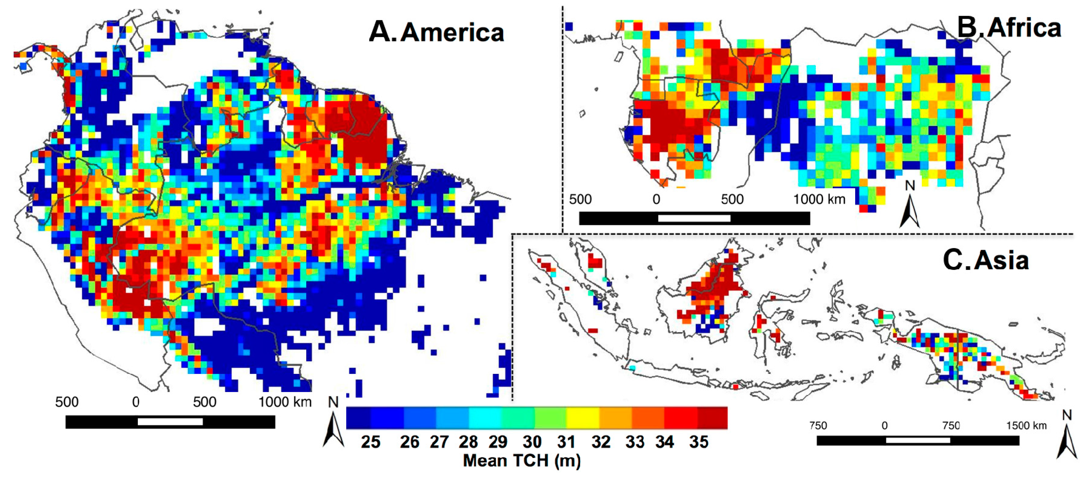
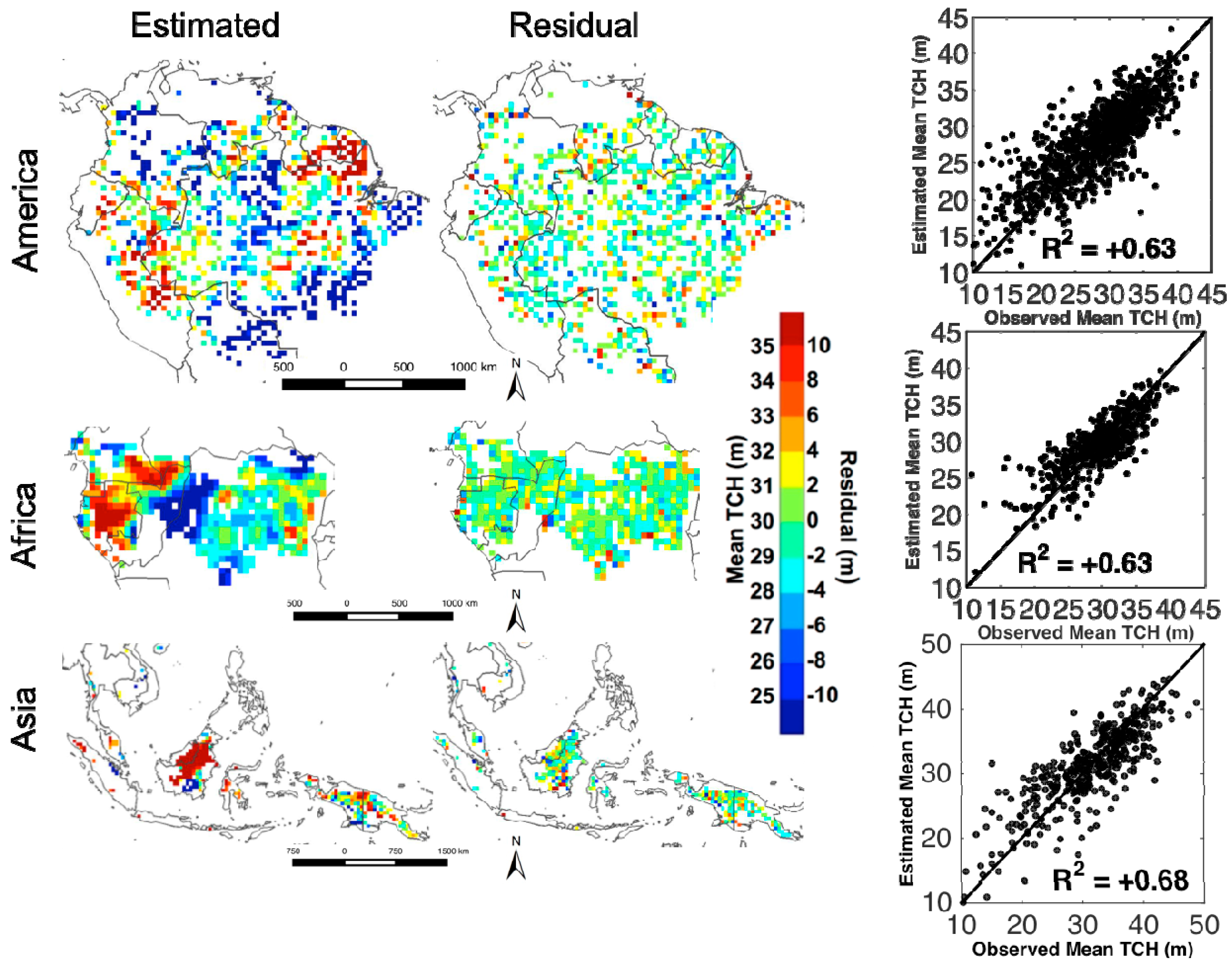
3.1. Spatial Patterns

The macroscale patterns of TCHm shown in the 0.5-deg gridded map (Figure 1) capture the known large-scale variations in forest structure along soil, elevation and climate gradients across three continents [1]. The Amazon region shows an overall lower TCHm and TCH90 (Figure 1 and Figure S4) than the forests in Africa and Asia, with a large fraction of forest in the Amazon having TCHm between 25 and 35 m. Forests in the central drainage system of the Amazon basin, distributed west of Rio Negro and the north and south of the Solomois River have on average 2 m shorter trees than forests surrounding it. The tallest forests, prominently visible in the TCH90 map, are located in the central east, northeast, and the southwest Amazonia in the state of Acre and southern Peru (Figure S4A). Tree height gradually decreases by going south to regions near the arc of deforestation and fragmented landscapes or in transitional semi-deciduous forests between Amazonia and Cerrado.
Tree height in western landscapes of the Central Africa, particularly in central and western Gabon grow taller than most regions in the African humid tropical forests, whereas trees in the central Congo Basin are on the average 2–4 m lower with TCHm ranging between 28 and 30 m (Figure S4B). Forests in Asia show the highest TCHm and TCH90 of all continents, especially in Malaysia, Kalimantan, Papua and some regions of Myanmar with TCHm often exceeding 32 m (Figure 1) and TCH90 reaching values >50 m (Figure S4C) on the average in the grid cells.
As a comparison, we created a stratified map separating potential ecoregions based on the 1-km gridded data of soil, ground elevation, land cover, and vegetation fractional cover maps (Supplementary S1; Tables S1 and S2). We used the GLAS lidar shots in each strata or ecoregion to create the mean TCH (Figure S7). This map shows finer features and variations when compared to the gridded TCH of coarser resolution (Figure 1), and also has an advantage of capturing the mean TCH under similar environmental factors. For example, inundated forests of the central Amazonia and along the river systems with average tree height of less than 25 m are separated (Figure S7B), while similar patterns are not readily visible in the gridded data (Figure 1). On the other hand, any spatial variation of TCH at pixel level vanishes and only a single measure exists for each strata, e.g., the vast region of western Amazon stratified as one ecoregion with one mean TCH (Supplementary S1; Figures S8 and S9), comparing to the gridded map (Figure 1) exhibiting a high contrast between the north and the south. Although the ecoregion-based map has its own merits, we decided to use the gridded map for further statistical analyses for its much larger sample size (in total 3119 gridded cells vs. 348 strata).

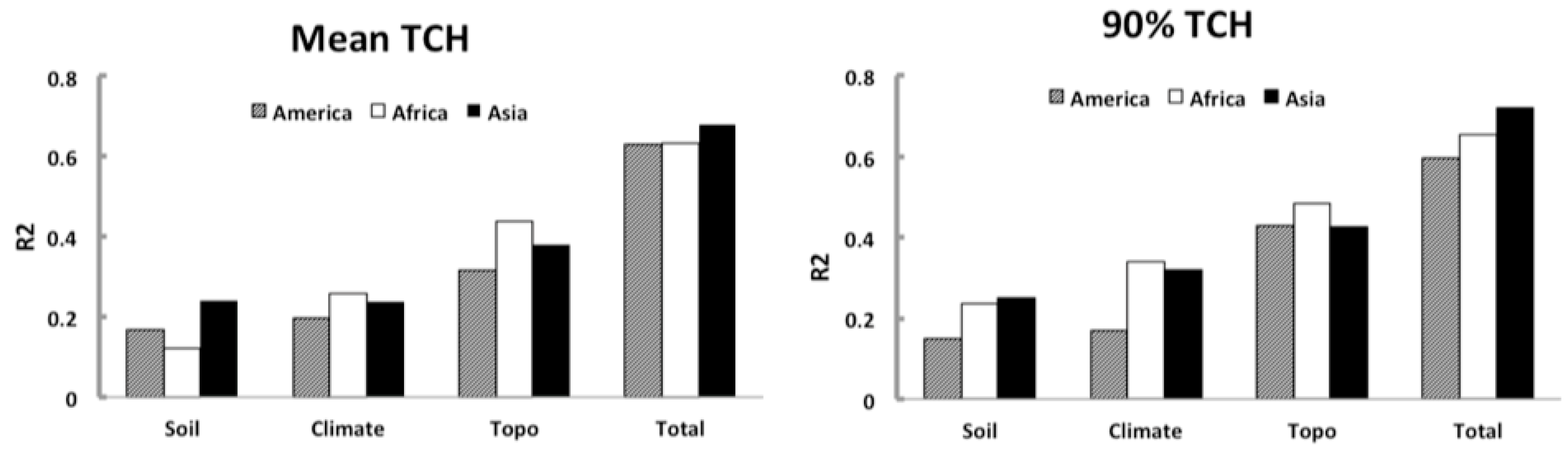
3.2. Statistical Analysis

Using spatial regression models, we estimated the tree height variations from the linear combination of environmental variables, thus explaining the first-order changes of forest tree heights with climate, soil and topographic features. With the help of landscape spatial features such as surface elevation and the contextual information from spatial correlation of pixels, the model can explain 63% of the variations in mean forest height (TCHm) using environmental variables in America and Africa, and about 68% of the variation in Asia (Figure 2). For the variability of large trees represented by TCH90, the explanatory power is less in America (60%), while the model performance improved in Asia (72%). The residual figures show that there is still a slight bias toward overestimation of short trees and underestimation of tall trees using environmental variables and regression model. Nevertheless, these spatial-based analyses successfully remove spatial autocorrelations (Figure S10) between geographically close pixels, which can help to correctly interpret the results of statistical regressions between forest height and various environmental inputs. We also found similar results using GLS spatial regression (Supplementary S2, Figure S11, Tables S3–S5). From partial linear regressions using SEVM, both TCHm and TCH90 are found to be mostly influenced by the landscape spatial features. The climate and soil together explain more than 30% of the variations in forest height (31% in America, 30% in Africa, and 47% in Asia), with climate variables having slightly higher explanatory power than soil properties (Figure 3).

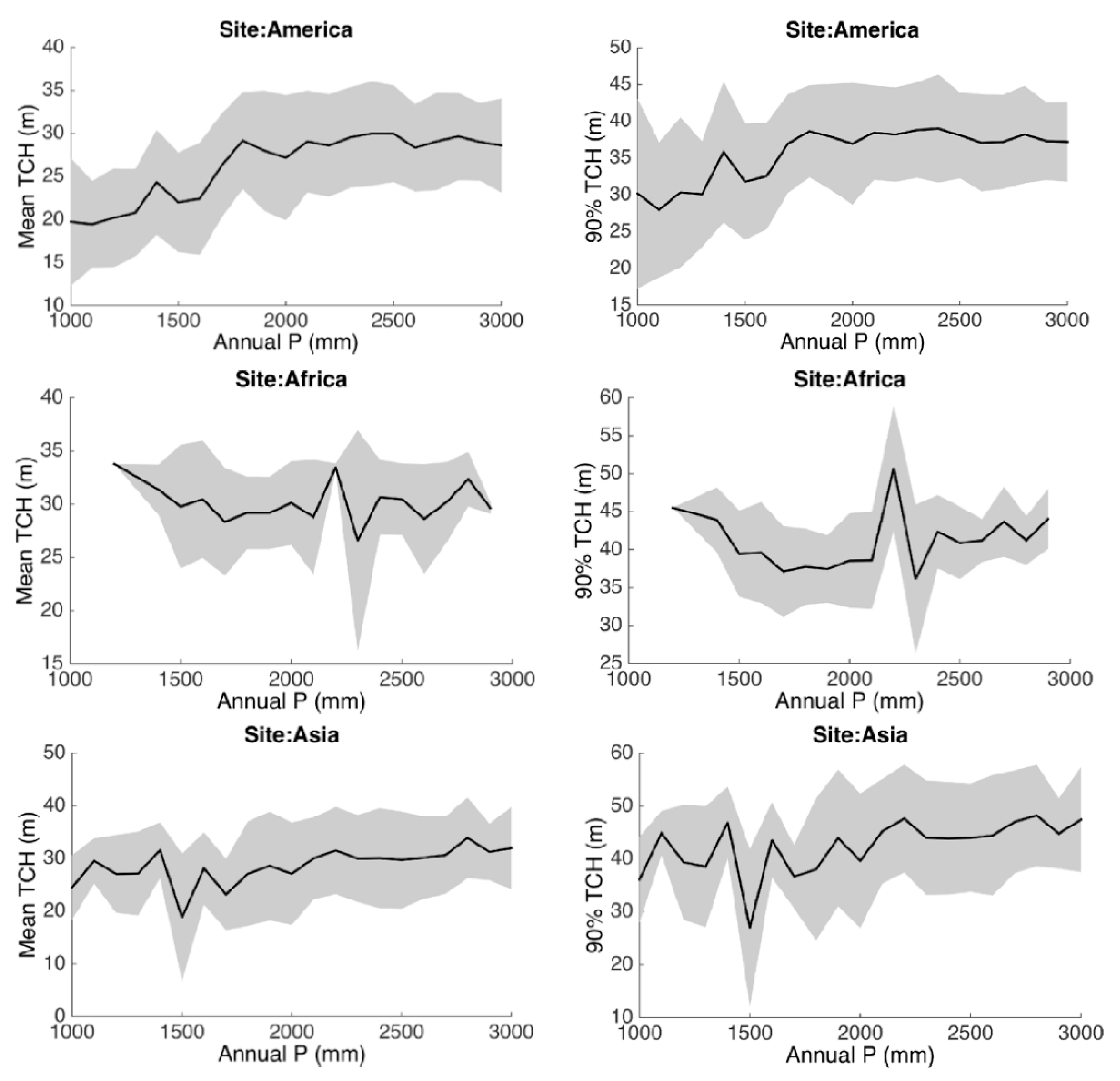
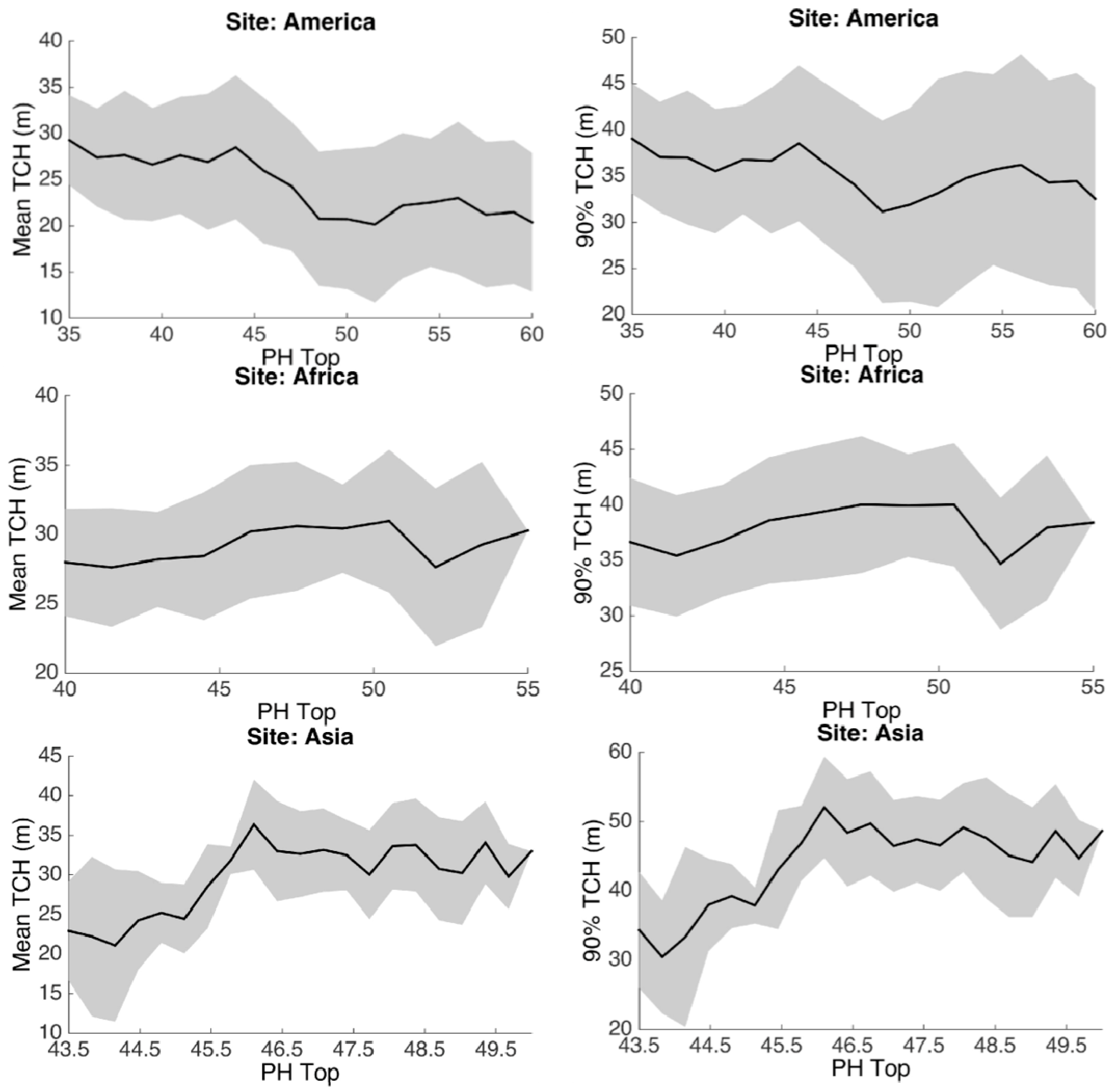
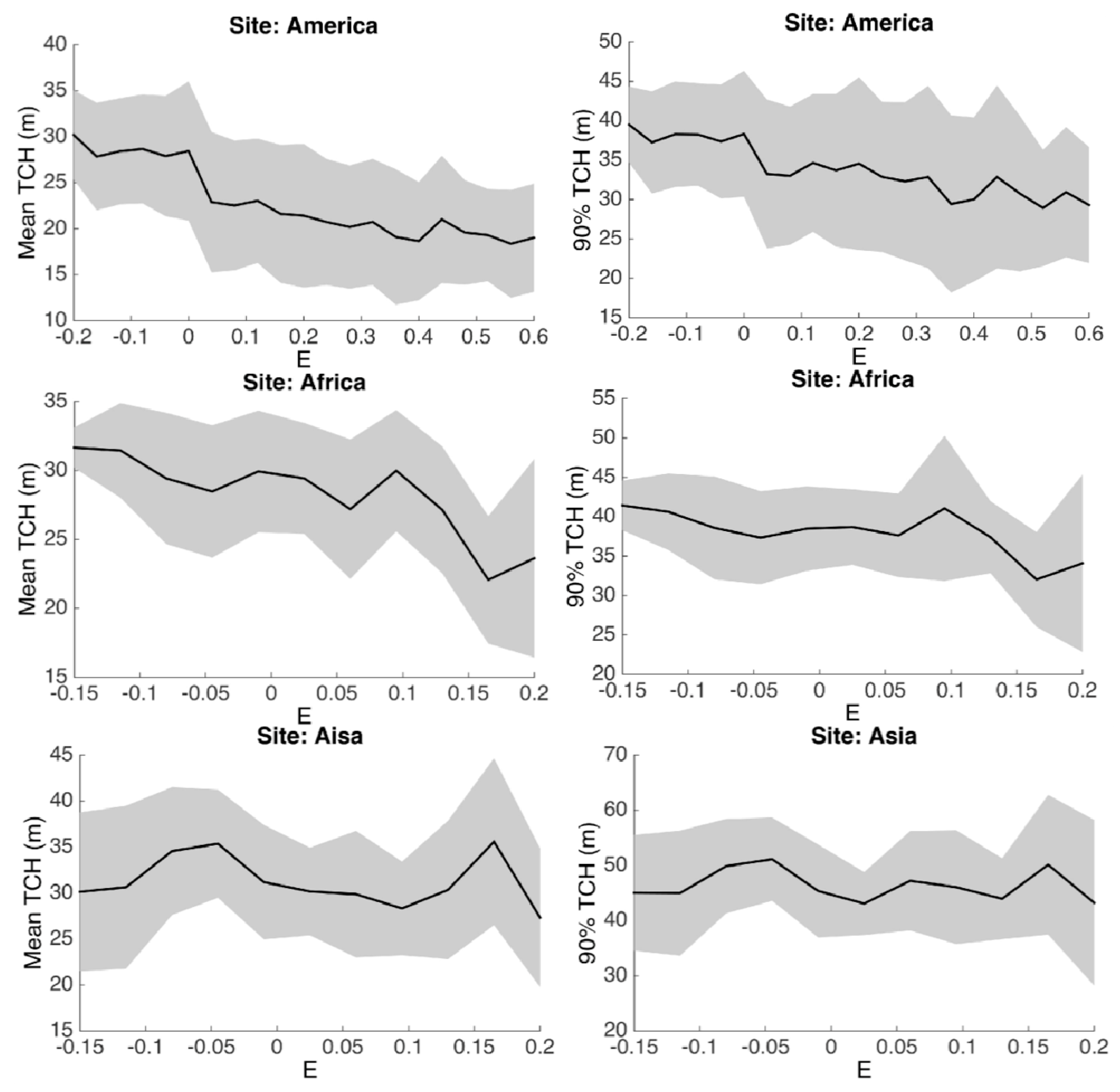
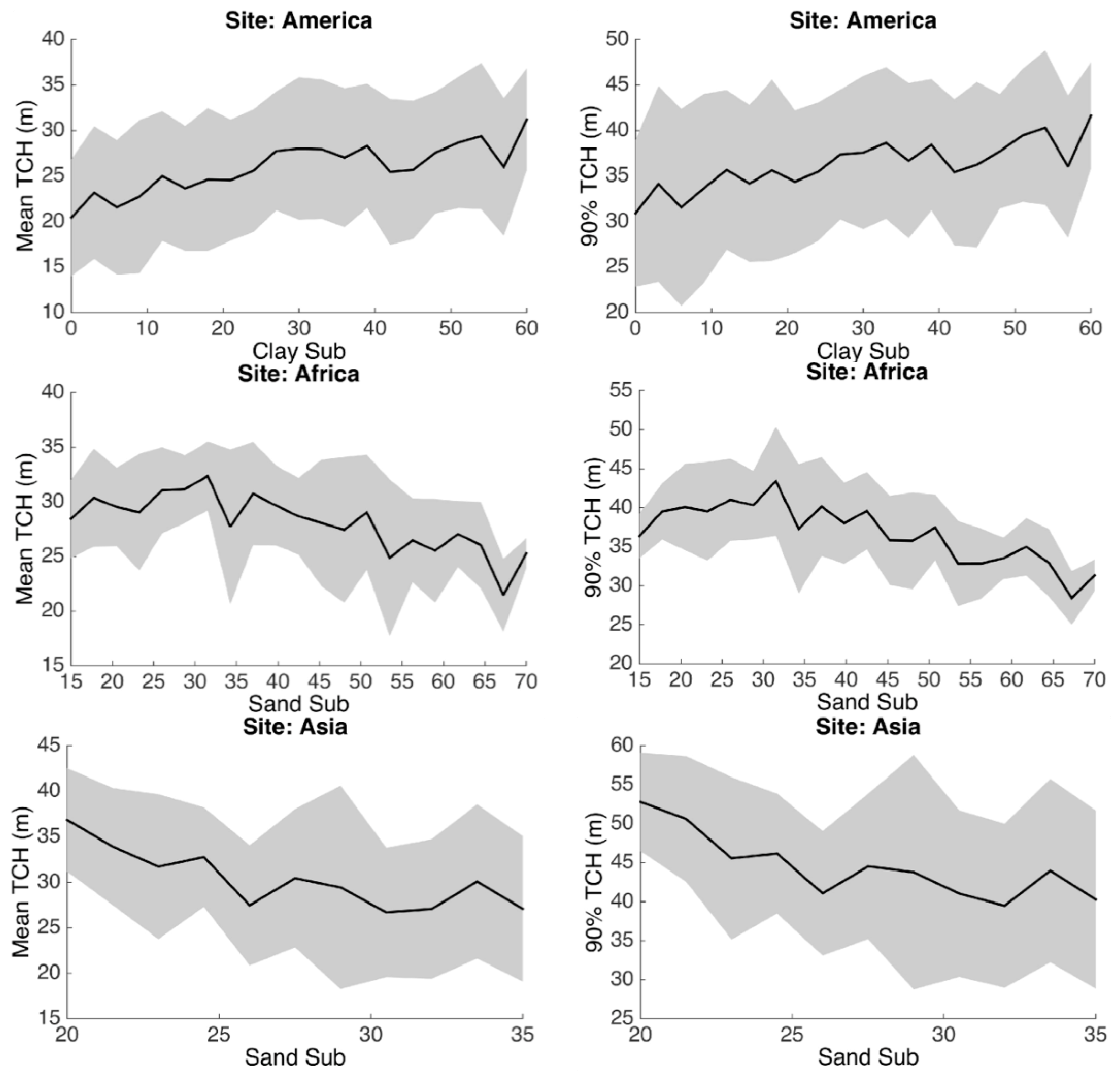
3.3. Environmental Controls

We identified environmental variables that are significantly correlated with spatial variations of TCH (Table 2 and Table 3). Among climate variables, the bioclimatic stress variable E shows high sensitivity to TCH90 variations across all continents, whereas it shows less significant sensitivity to variations of TCHm. The importance of seasonality of climate in explaining tree height growth and spatial variations are shown in terms of different precipitation variables. For American and African forests, precipitation of driest quarter is correlated with variations of TCH90 suggesting strong influence on tree growth. In Asia, the seasonality of precipitation is negatively correlated with TCH90 indicating taller forests growing in areas with more climate stability throughout the year and with less seasonality. Seasonality of precipitation has slightly less effect on the average forest height (TCHm) except in Asia with similar explanatory power as for TCH90.
Terrain elevation heterogeneity or ruggedness represented by STRM SD variable is positively correlated with TCH variation across all continents in both methods, indicating that the ruggedness is much more important than the average ground elevation in tree height distributions. This variable strongly influenced the distribution of dominant forest height (TCH90) in America and Africa and has the largest coefficient compared to other predictor variables (Table 3). However, the same is not true about TCHm, expect with some statistical significance in Africa, suggesting that moderate ruggedness of the landscape impact the dominant tree height more than the average height.
Soil properties have less influence on variations of TCH compared to either the climate or the geographical features. However, individual properties present nonnegligible impacts on TCH variations. Clay content, as a physical structural property of soil, exhibits a significantly positive relationship to both TCH metrics in all continents. Cation-exchange capacity (CEC), a well-known chemical property and a measure of soil fertility, is also a significant factor in Africa and Asia for TCHm, and in America and Asia for TCH90. A general chemical measure, pH value, shows significant but completely opposite effects on TCH metrics in America than other continents, with pH value negatively correlated to TCHm and TCH90 in Americas, but positively correlated in Africa and Asia. For other soil biological properties, we find that the soil organic carbon (OC) content has a strong negative correlation on TCH metrics in America, while it shows positively correlated with TCHm in Africa, and less clear in Asia.

4. Discussion

Results from our study suggest that mean annual properties of climate in humid tropical regions such as annual mean and total precipitation do not exert any significant control or limit both the mean and 90 percentile of forest canopy height across the three continents. Similarly, annual mean temperature has no significant effect on the mean tree height variations. Our findings suggest that the spatial distribution of mean canopy structure in humid tropical forests are not strongly dependent on the mean climate characteristics. Although the relationship between TCH metrics and annual precipitation (Figure 4) demonstrate that TCH metrics increase with rainfall within a certain precipitation range (1000 mm to 2000 mm), particularly in the American forests, most observations from humid tropical forests are located in the plateau area (precipitation > 2000 mm), thus making these mean/total climate variables less important compared to other climate variables such as seasonality parameters and extreme values. Note that in the model selection process, mean climate variables were rarely included as important predictor variables (except in the case of TCHm in America).
Climate seasonality is one of the major factors regulating the maximum or dominant forest height represented by TCH90 (Table 3). Particularly, the E variable representing the water deficit, ranks 4th in America, 2nd in Africa, and 2nd in Asia as the set of predictor variables (excluding the spatial features) in the SEVM approach. The water deficit (E variable) also has a significant impact on the TCHm in America and Africa. Precipitation Seasonality, replacing the E variable in Asia, is found to be the important factor influencing the forest mean height (Table 2). By plotting the TCH metrics directly against the E factor (Figure 5), we found a consistently negative relationship in either America or Africa, but a less clear pattern in Asia, suggesting that water deficit plays a key control in distribution of tree height in continental tropical forests. The island geography in southeast Asia moderates the temperature seasonality [53] while still provides vital seasonal rainfalls from monsoon phenomenon [54], so that the precipitation seasonality has a larger influence and dominates the changes of E variable in Asia. Our study suggests that at the macroscale, the seasonal variation of climate, particularly precipitation-related, is one of the most important factors linearly relating to mean and dominant forest height as forest structural traits.
Spatial regression results also show that the extreme values of precipitation (P coldest Q, P warmest Q, P driest M, P driest Q and P wettest M) are more important than the extreme values of temperature (M T warmest Q, Max T warmest m, M T driest Q, and Min T coldest m) in macroscale patterns of mean forest height in tropics (Table 2 and Table 3). Partial R2 results of TCHm show that the extreme values of precipitation can explain 4 to 12 times more than the extreme values of temperature in America and Asia, while the extreme values play an equal role in African forests. This result confirms that tropical forests are more sensitive to precipitation-related extreme events, such as droughts, rather than temperature-induced events in their present condition [13]. However, this does not necessarily imply that changes in future temperature due to climate warming do not have any adverse effects on tropical forest function. There are strong evidence that climate warming is associated with changes of precipitation seasonality and drier conditions with strong influence of the patterns and processes that sustain tropical forests [55,56,57]. In fact, the gridded maximum height of the forests when used as a surrogate for the maximum attainable height of tree population in the forest, may be strongly related to demographic trade-offs and the recruitment rate efficiency, together reflecting the investments for hydraulic conductance of forests in the region [26,58]. Sensitivity of the maximum height trait to climate over the tropics suggests that changes of the climate, particularly precipitation seasonality may directly impact demographical trade-offs such as mortality and recruitment rates. These effects will potentially change the tree composition by emphasizing the abundance of trees with more efficient hydraulic conductivity and possibly shorter in height [59].
Recent studies of modeling efforts on the prediction of tropical forest biomass and productivity always present a biased estimation of large trees due to the limited or simplified resource information regulating the growth of forest [60]. We thus included the soil properties in our analyses and attempted to find evidences of edaphic controls on tropical tree height. Although the overall importance of soil on TCH is approximately half of that of climate (Figure 3), the TCH variations are statistically related to the changes of soil properties. In all regression results, TCHm and TCH90 show a significantly positive relationship to the soil physical property–clay content of either topsoil or subsoil. The results support the typical functionality of clay content in soil that (1) it has a relatively large nutrient capacity; (2) it can hold enough water for root absorption, and (3) it potentially has the structural strength to fix the roots of large trees [61]. The one-to-one relationships of TCH and soil physical property demonstrate a positive trend of TCH with clay content in America, as well as a negative relationship between TCH and sand in Africa and Asia (Figure 6). We plotted sand instead of clay content in Africa and Asia due to the fact that clay content has less dynamic ranges in these two continents. However, the variation of sand content should compensate the changes of clay, as sand, silt and clay together describe the soil texture. Another significant control of the soil is the negative relationship between TCHm and the soil fertility–CEC. It is seemingly counterintuitive, that mature forests with taller trees are actually located on less fertile soil. However, the result is corroborated by several previous findings in the Amazon basin–forests with largest above ground biomass occur on relatively poor soils [17]. Although the total CEC may not be an ideal indicator of fertility due to the inclusion of aluminum, such negative relationship can potentially be explained by the faster turnover rates for forests with high soil fertility [17]. In contrast, we found positive relationships between pH values and TCHm both Africa and Asia, though CEC should be highly dependent on the pH values. We also found this behavior of pH by plotting the one-to-one relationships of TCH vs pH values (Figure 7). The underlying reasons for these differences remain unclear. Possible explanation could be that the forests in Africa and Asia are in favor of the basic environment to allow more base cations (Ca, Mg, K and Na) rather than Al and H+ ions under high acidity, which may be explained by the less factions of Ferralsol found in Africa and Asia [62]. If we consider the combined effect of pH and CEC as the indicator of the soil fertility, then similar observations on the continental differences have been reported in other studies [63]. The last soil factor that can explain the TCH distribution at macroscale is the soil organic carbon (OC). Interestingly, the sensitivity of OC to TCH varies continent by continent. In America, OC is negatively related to both TCHm and TCH90, while it is positively correlated to TCHm in Africa. In addition, these relationships are less obvious for the TCH90 in either Africa or Asia.
The last control variable on forest structure we tested is ground topography. Higher elevation usually indicates lower temperature and probably less water availability, leading to a high possibility of resource limitation. Thus, SRTM is expected to show a negative relationship to TCH metrics, like what we found in Table 2 and Table 3 for most of the SRTM numbers. However, most of them are not significant, either meaning the mean ground elevation is not one of the major drivers for TCH prediction, or insufficient data range due to the fact that most observations are from low-elevation inundated forests. In contrast, the standard deviation of ground elevation (SRTM SD) consistently shows a positive relationship to either TCHm or TCH90 and statistically significant in Africa and America, indicating that the surface ruggedness is more important in finding taller trees, or old and tall trees are better preserved in hard-reaching (rugged) area. Such regional differences imply that areas with moderate topography can produce a higher overall carbon stock probably due to its large variation in resource supply.
In our analysis the underestimation of TCH using climate-only data is not resolved. In fact, we can see both underestimation of high TCH and overestimation of low TCH, suggested by the regressions analyses (Figure 2). This is probably due to: (1) land use changes creating heterogeneous and fragmented landscapes with variations in tree height at small scale that are not captured by the land cover map but can be detected by lidar footprints. Although we filtered the GLAS lidar based on the land cover types, but a significant number of GLAS footprints over fragmented landscapes may still remain in the mix; (2) there are other controls not considered in this analysis, such as disturbances including logging, disease and wildfires, that drive the growth of tall trees. Essentially, tree height is related to its age, especially when the tree is not mature yet. The forest turnover rate is high in areas where it is easily accessible (close to road, river, population, or in low elevation) [64]. Given the same conditions of climate, soil and topographic features, the areas with high disturbances could have lower tree heights that are not detectable from our current regression model.

5. Conclusions

The macroscale variations of tree height over humid tropical forests present regionally as well as continentally different patterns from systematically samples of satellite observations using GLAS lidar sensors. In this study, we used TCHm and TCH90 derived from GLAS to analyze the regional variability of average and large trees globally. Using spatial regression, our continental-scale results confirm other landscape and regional studies that soil fertility, geology and climate may jointly control majority of the regional variations of tropical forest structure and influence both biomass stocks and dynamics. Our tests include a large suite of parameters in climate and soil properties, which can provide as a source of reference to other in-depth studies focusing on the unexplainable fraction of variations caused by other environmental factors, such as biotic and disturbance regimes, not included in this study.

Supplementary Materials

The following materials are available online at www.mdpi.com/2072-4292/8/6/494/s1, Supplementary S1: Ecoregion-based Stratification, Supplementary S2. Comparative Spatial Regression Results, Figure S1: Systematic sampling of GLAS lidar shots over tropics, Figure S2: Compassion of vertical profiles between GLAS points and associated Airborne lidar points in three continents, Figure S3: Vertical profile of the GLAS footprints in three continents, Figure S4: TCH90 calculated from GLAS dataset in 0.5-deg resolution, Figure S5: Relationship between TCHm using all GLAS points and TCHm from random sampling, Figure S6: Diagram of the processing steps of spatial regression analysis, Figure S7: Mean TCH calculated from GLAS dataset Based on Soil types, Figure S8: The tropical soil classification map, Figure S9: Diagram of the ecoregion classification, Figure S10: Spatial autocorrelations in terms of Moran’s I, Figure S11. Spatial regression results using GLS, Table S1: Soil classification used in the ecoregion stratification in the tropics, Table S2: Separation of Ferralsols soil type into 7 classes in the African forests, Table S3: Spatial regression results using GLS method for TCHm, Table S4: Spatial regression results using GLS method for TCH90, Table S5: Example regression coefficients table of TCHm using SEVM method in Africa.

Acknowledgments

The research was funded by Gabon National Park (ANPN) under the contract of 011-ANPN/2012/SE-LJTW at UCLA. We thank IIASA, FAO, USGS, NASA, Worldclim science teams for making their data available.

Author Contributions

Sassan S. Saatchi designed the study. Yifan Yu and Michael A. Lefsky provided the GLAS data set developed for tropical forest studies. Yan Yang processed and analyzed data. Sassan S. Saatchi, Liang Xu and Yan Yang drafted the manuscript. All authors contributed with ideas, writing and discussions.

Conflicts of Interest

The authors declare no conflict of interest.

References

  1. Saatchi, S.S.; Harris, N.L.; Brown, S.; Lefsky, M.; Mitchard, E.T.; Salas, W.; Zutta, B.R.; Buermann, W.; Lewis, S.L.; Hagen, S. Benchmark map of forest carbon stocks in tropical regions across three continents. Proc. Natl. Acad. Sci. USA 2011, 108, 9899–9904. [Google Scholar] [CrossRef] [PubMed]
  2. Pan, Y.; Birdsey, R.A.; Fang, J.; Houghton, R.; Kauppi, P.E.; Kurz, W.A.; Phillips, O.L.; Shvidenko, A.; Lewis, S.L.; Canadell, J.G.; et al. A large and persistent carbon sink in the world’s forests. Science 2011, 333, 988–993. [Google Scholar] [CrossRef] [PubMed]
  3. Baker, T.R.; Phillips, O.L.; Malhi, Y.; Almeida, S.; Arroyo, L.; Di Fiore, A.; Erwin, T.; Killeen, T.J.; Laurance, S.G.; Laurance, W.F.; et al. Variation in wood density determines spatial patterns in Amazonian forest biomass. Glob. Chang. Biol. 2004, 10, 545–562. [Google Scholar] [CrossRef]
  4. Phillips, O.L.; Aragão, L.E.O.C.; Lewis, S.L.; Fisher, J.B.; Lloyd, J.; López-González, G.; Malhi, Y.; Monteagudo, A.; Peacock, J.; Quesada, C.A.; et al. Drought sensitivity of the amazon rainforest. Science 2009, 323, 1344–1347. [Google Scholar] [CrossRef] [PubMed] [Green Version]
  5. Asner, G.P.; Mascaro, J.; Anderson, C.; Knapp, D.E.; Martin, R.E.; Kennedy-Bowdoin, T.; van Breugel, M.; Davies, S.; Hall, J.S.; Muller-Landau, H.C.; et al. High-fidelity national carbon mapping for resource management and REDD+. Carbon Balance Manag. 2013, 8, 1–14. [Google Scholar] [CrossRef] [PubMed]
  6. Clark, D.A.; Clark, D.B.; Oberbauer, S.F. Field-quantified responses of tropical rainforest aboveground productivity to increasing CO2 and climatic stress, 1997–2009. J. Geophys. Res. Biogeosci. 2013, 118, 783–794. [Google Scholar] [CrossRef]
  7. Espírito-Santo, F.D.B.; Gloor, M.; Keller, M.; Malhi, Y.; Saatchi, S.; Nelson, B.; Junior, R.C.O.; Pereira, C.; Lloyd, J.; Frolking, S.; et al. Size and frequency of natural forest disturbances and the Amazon forest carbon balance. Nat. Commun. 2014, 5. [Google Scholar] [CrossRef] [PubMed]
  8. Malhi, Y.; Doughty, C.E.; Goldsmith, G.R.; Metcalfe, D.B.; Girardin, C.A.J.; Marthews, T.R.; del Aguila-Pasquel, J.; Aragão, L.E.O.C.; Araujo-Murakami, A.; Brando, P.; et al. The linkages between photosynthesis, productivity, growth and biomass in lowland Amazonian forests. Glob. Chang. Biol. 2015, 21, 2283–2295. [Google Scholar] [CrossRef] [PubMed]
  9. Marvin, D.C.; Asner, G.P.; Knapp, D.E.; Anderson, C.B.; Martin, R.E.; Sinca, F.; Tupayachi, R. Amazonian landscapes and the bias in field studies of forest structure and biomass. Proc. Natl. Acad. Sci. USA 2014, 111, E5224–E5232. [Google Scholar] [CrossRef] [PubMed]
  10. Saatchi, S.; Mascaro, J.; Xu, L.; Keller, M.; Yang, Y.; Duffy, P.; Espírito-Santo, F.; Baccini, A.; Chambers, J.; Schimel, D. Seeing the forest beyond the trees. Glob. Ecol. Biogeogr. 2015, 24, 606–610. [Google Scholar] [CrossRef]
  11. Frolking, S.; Palace, M.W.; Clark, D.B.; Chambers, J.Q.; Shugart, H.H.; Hurtt, G.C. Forest disturbance and recovery: A general review in the context of spaceborne remote sensing of impacts on aboveground biomass and canopy structure. J. Geophys. Res. Biogeosci. 2009, 114, G00E02. [Google Scholar] [CrossRef]
  12. Chambers, J.Q.; Negron-Juarez, R.I.; Marra, D.M.; Vittorio, A.D.; Tews, J.; Roberts, D.; Ribeiro, G.H.P.M.; Trumbore, S.E.; Higuchi, N. The steady-state mosaic of disturbance and succession across an old-growth Central Amazon forest landscape. Proc. Natl. Acad. Sci. USA 2013, 110, 3949–3954. [Google Scholar] [CrossRef] [PubMed]
  13. Saatchi, S.; Asefi-Najafabady, S.; Malhi, Y.; Aragão, L.E.O.C.; Anderson, L.O.; Myneni, R.B.; Nemani, R. Persistent effects of a severe drought on Amazonian forest canopy. Proc. Natl. Acad. Sci. USA 2013, 110, 565–570. [Google Scholar] [CrossRef] [PubMed]
  14. Tian, H.; Melillo, J.M.; Kicklighter, D.W.; McGuire, A.D.; Helfrich, J.V.K.; Moore, B.; Vörösmarty, C.J. Effect of interannual climate variability on carbon storage in Amazonian ecosystems. Nature 1998, 396, 664–667. [Google Scholar] [CrossRef]
  15. Malhi, Y.; Roberts, J.T.; Betts, R.A.; Killeen, T.J.; Li, W.; Nobre, C.A. Climate change, deforestation, and the fate of the Amazon. Science 2008, 319, 169–172. [Google Scholar] [CrossRef] [PubMed]
  16. Higgins, M.A.; Asner, G.P.; Perez, E.; Elespuru, N.; Tuomisto, H.; Ruokolainen, K.; Alonso, A. Use of Landsat and SRTM data to detect broad-scale biodiversity patterns in northwestern Amazonia. Remote Sens. 2012, 4, 2401–2418. [Google Scholar] [CrossRef]
  17. Quesada, C.A.; Phillips, O.L.; Schwarz, M.; Czimczik, C.I.; Baker, T.R.; Patiño, S.; Fyllas, N.M.; Hodnett, M.G.; Herrera, R.; Almeida, S.; et al. Basin-wide variations in Amazon forest structure and function are mediated by both soils and climate. Biogeosciences 2012, 9, 2203–2246. [Google Scholar] [CrossRef] [Green Version]
  18. Webb, C.; Cannon, C.; Davies, S. Ecological organization, biogeography, and the phylogenetic structure of tropical forest tree communities. In Tropical Forest Community Ecology; Carson, W., Schnitzer, S., Eds.; Blackwell: Malden, MA, USA, 2008; pp. 79–97. [Google Scholar]
  19. Kembel, S.W.; Hubbell, S.P. The phylogenetic structure of a Neotropical forest tree community. Ecology 2006, 87, S86–S99. [Google Scholar] [CrossRef]
  20. Iida, Y.; Poorter, L.; Sterck, F.; Kassim, A.R.; Potts, M.D.; Kubo, T.; Kohyama, T.S. Linking size-dependent growth and mortality with architectural traits across 145 co-occurring tropical tree species. Ecology 2014, 95, 353–363. [Google Scholar] [CrossRef] [PubMed]
  21. Feldpausch, T.R.; Lloyd, J.; Lewis, S.L.; Brienen, R.J. W.; Gloor, M.; Monteagudo Mendoza, A.; Lopez-Gonzalez, G.; Banin, L.; Abu Salim, K.; Affum-Baffoe, K.; et al. Tree height integrated into pantropical forest biomass estimates. Biogeosciences 2012, 9, 3381–3403. [Google Scholar] [CrossRef] [Green Version]
  22. Banin, L.; Feldpausch, T.R.; Phillips, O.L.; Baker, T.R.; Lloyd, J.; Affum-Baffoe, K.; Arets, E.J.M.M.; Berry, N.J.; Bradford, M.; Brienen, R.J.W.; et al. What controls tropical forest architecture? Testing environmental, structural and floristic drivers. Glob. Ecol. Biogeogr. 2012, 21, 1179–1190. [Google Scholar] [CrossRef]
  23. DeWalt, S.J.; Chave, J. Structure and biomass of four lowland Neotropical Forests. Biotropica 2004, 36, 7–19. [Google Scholar] [CrossRef]
  24. Moser, B.; Fridley, J.D.; Askew, A.P.; Grime, J.P. Simulated migration in a long-term climate change experiment: invasions impeded by dispersal limitation, not biotic resistance. J. Ecol. 2011, 99, 1229–1236. [Google Scholar] [CrossRef]
  25. Slik, J.W.F.; Paoli, G.; McGuire, K.; Amaral, I.; Barroso, J.; Bastian, M.; Blanc, L.; Bongers, F.; Boundja, P.; Clark, C.; et al. Large trees drive forest aboveground biomass variation in moist lowland forests across the tropics. Glob. Ecol. Biogeogr. 2013, 22, 1261–1271. [Google Scholar] [CrossRef]
  26. Kohyama, T.; Suzuki, E.; Partomihardjo, T.; Yamada, T.; Kubo, T. Tree species differentiation in growth, recruitment and allometry in relation to maximum height in a Bornean mixed dipterocarp forest. J. Ecol. 2003, 91, 797–806. [Google Scholar] [CrossRef]
  27. Lefsky, M.A. A global forest canopy height map from the Moderate Resolution Imaging Spectroradiometer and the Geoscience Laser Altimeter System. Geophys. Res. Lett. 2010, 37, L15401. [Google Scholar] [CrossRef]
  28. Le Toan, T.; Quegan, S.; Davidson, M.W.J.; Balzter, H.; Paillou, P.; Papathanassiou, K.; Plummer, S.; Rocca, F.; Saatchi, S.; Shugart, H.; et al. The BIOMASS mission: Mapping global forest biomass to better understand the terrestrial carbon cycle. Remote Sens. Environ. 2011, 115, 2850–2860. [Google Scholar] [CrossRef]
  29. Saatchi, S.S.; Marlier, M.; Chazdon, R.L.; Clark, D.B.; Russell, A.E. Impact of spatial variability of tropical forest structure on radar estimation of aboveground biomass. Remote Sens. Environ. 2011, 115, 2836–2849. [Google Scholar] [CrossRef]
  30. Bontemps, S.; Defourny, P.; Van Bogaert, E.; Arino, O.; Kalogirou, V.; Ramos Perez, J. GlobCover 2009: Products Description and Validation Report; UCLouvain & ESA: Louvain-la-Neuve, Belgium, 2011. [Google Scholar]
  31. Abshire, J.B.; Sun, X.; Riris, H.; Sirota, J.M.; McGarry, J.F.; Palm, S.; Yi, D.; Liiva, P. Geoscience Laser Altimeter System (GLAS) on the ICESat Mission: On-orbit measurement performance. Geophys. Res. Lett. 2005, 32, L21S02. [Google Scholar] [CrossRef]
  32. Lefsky, M.A.; Harding, D.J.; Keller, M.; Cohen, W.B.; Carabajal, C.C.; Espirito-Santo, F.D.B.; Hunter, M.O.; de Oliveira, R., Jr. Estimates of forest canopy height and aboveground biomass using ICESat. Geophys. Res. Lett. 2005, 32, L22S02. [Google Scholar] [CrossRef]
  33. Sun, G.; Ranson, K.J.; Kimes, D.S.; Blair, J.B.; Kovacs, K. Forest vertical structure from GLAS: An evaluation using LVIS and SRTM data. Remote Sens. Environ. 2008, 112, 107–117. [Google Scholar] [CrossRef]
  34. Lefsky, M.A.; Keller, M.; Pang, Y.; De Camargo, P.B.; Hunter, M.O. Revised method for forest canopy height estimation from Geoscience Laser Altimeter System waveforms. J. Appl. Remote Sens. 2007, 1. [Google Scholar] [CrossRef]
  35. Lim, K.; Treitz, P.; Wulder, M.; St-Onge, B.; Flood, M. Lidar remote sensing of forest structure. Prog. Phys. Geogr. 2003, 27, 88–106. [Google Scholar] [CrossRef]
  36. Van Leeuwen, M.; Nieuwenhuis, M. Retrieval of forest structural parameters using Lidar remote sensing. Eur. J. For. Res. 2010, 129, 749–770. [Google Scholar] [CrossRef]
  37. Rabus, B.; Eineder, M.; Roth, A.; Bamler, R. The shuttle radar topography mission—A new class of digital elevation models acquired by spaceborne radar. ISPRS J. Photogramm. Remote Sens. 2003, 57, 241–262. [Google Scholar] [CrossRef]
  38. Farr, T.G.; Rosen, P.A.; Caro, E.; Crippen, R.; Duren, R.; Hensley, S.; Kobrick, M.; Paller, M.; Rodriguez, E.; Roth, L.; et al. The shuttle radar topography mission. Rev. Geophys. 2007, 45, RG2004. [Google Scholar] [CrossRef]
  39. Hijmans, R.J.; Cameron, S.E.; Parra, J.L.; Jones, P.G.; Jarvis, A. Very high resolution interpolated climate surfaces for global land areas. Int. J. Climatol. 2005, 25, 1965–1978. [Google Scholar] [CrossRef]
  40. Synes, N.W.; Osborne, P.E. Choice of predictor variables as a source of uncertainty in continental-scale species distribution modelling under climate change. Glob. Ecol. Biogeogr. 2011, 20, 904–914. [Google Scholar] [CrossRef]
  41. Nachtergaele, F.O.F.; Licona-Manzur, C. The Land Degradation Assessment in Drylands (LADA) Project: reflections on indicators for land degradation assessment. In The Future of Drylands; Lee, C., Schaaf, T., Eds.; Springer Netherlands: Tunis, Tunisia, 2008; pp. 327–348. [Google Scholar]
  42. Chave, J.; Réjou-Méchain, M.; Búrquez, A.; Chidumayo, E.; Colgan, M.S.; Delitti, W.B.C.; Duque, A.; Eid, T.; Fearnside, P.M.; Goodman, R.C.; et al. Improved allometric models to estimate the aboveground biomass of tropical trees. Glob. Chang. Biol. 2014, 20, 3177–3190. [Google Scholar] [CrossRef] [PubMed]
  43. FAO/IIASA/ISRIC/ISSCAS/JRC. Harmonized World Soil Database (Version 1.2); FAO: Rome, Italy, 2012. [Google Scholar]
  44. Dormann, C.F.; McPherson, J.M.; Araújo, M.B.; Bivand, R.; Bolliger, J.; Carl, G.; Davies, R.G.; Hirzel, A.; Jetz, W.; Daniel Kissling, W.; et al. Methods to account for spatial autocorrelation in the analysis of species distributional data: A review. Ecography 2007, 30, 609–628. [Google Scholar] [CrossRef]
  45. Mauricio Bini, L.; Diniz-Filho, J.A.F.; Rangel, T.F.L.V.B.; Akre, T.S.B.; Albaladejo, R.G.; Albuquerque, F.S.; Aparicio, A.; Araújo, M.B.; Baselga, A.; Beck, J.; et al. Coefficient shifts in geographical ecology: An empirical evaluation of spatial and non-spatial regression. Ecography 2009, 32, 193–204. [Google Scholar] [CrossRef]
  46. Rangel, T.F.; Diniz-Filho, J.A.F.; Bini, L.M. SAM: A comprehensive application for spatial analysis in macroecology. Ecography 2010, 33, 46–50. [Google Scholar] [CrossRef]
  47. Matula, D.W.; Sokal, R.R. Properties of Gabriel graphs relevant to geographic variation research and the clustering of points in the plane. Geogr. Anal. 1980, 12, 205–222. [Google Scholar] [CrossRef]
  48. Moran, P.A.P. Notes on continuous stochastic phenomena. Biometrika 1950, 37, 17–23. [Google Scholar] [CrossRef] [PubMed]
  49. Akaike, H. A new look at the statistical model identification. IEEE Trans. Autom. Control 1974, 19, 716–723. [Google Scholar] [CrossRef]
  50. Belsley, D.A.; Kuh, E.; Welsch, R.E. Regression Diagnostics: Identifying Influential Data and Sources of Collinearity; John Wiley & Sons: Hoboken, NJ, USA, 2005. [Google Scholar]
  51. Burnham, K.P.; Anderson, D.R.; Huyvaert, K.P. AIC model selection and multimodel inference in behavioral ecology: Some background, observations, and comparisons. Behav. Ecol. Sociobiol. 2011, 65, 23–35. [Google Scholar] [CrossRef]
  52. O’brien, R.M. A caution regarding rules of thumb for variance inflation factors. Qual. Quant. 2007, 41, 673–690. [Google Scholar] [CrossRef]
  53. Laing, A.; Evans, J.L. Introduction to Tropical Meteorology; University Corporation Atmospheric Research: Boulder, CO, USA, 2011. [Google Scholar]
  54. Bloom, D.E.; Sachs, J.D.; Collier, P.; Udry, C. Geography, demography, and economic growth in Africa. Brook. Pap. Econ. Act. 1998, 1998, 207–295. [Google Scholar] [CrossRef]
  55. Malhi, Y.; Saatchi, S.; Girardin, C.; AragãO, L.E.O.C. The production, storage, and flow of Carbon in Amazonian forests. In Amazonia and Global Change; Keller, M., Bustamante, M., Gash, J., Dias, P.S., Eds.; American Geophysical Union: Washington, DC, USA, 2009; pp. 355–372. [Google Scholar]
  56. Cox, P.M.; Pearson, D.; Booth, B.B.; Friedlingstein, P.; Huntingford, C.; Jones, C.D.; Luke, C.M. Sensitivity of tropical carbon to climate change constrained by carbon dioxide variability. Nature 2013, 494, 341–344. [Google Scholar] [CrossRef] [PubMed]
  57. Huntingford, C.; Zelazowski, P.; Galbraith, D.; Mercado, L.M.; Sitch, S.; Fisher, R.; Lomas, M.; Walker, A.P.; Jones, C.D.; Booth, B.B.B.; et al. Simulated resilience of tropical rainforests to CO2-induced climate change. Nat. Geosci. 2013, 6, 268–273. [Google Scholar] [CrossRef]
  58. Poorter, L. Leaf traits show different relationships with shade tolerance in moist versus dry tropical forests. New Phytol. 2009, 181, 890–900. [Google Scholar] [CrossRef] [PubMed]
  59. Engelbrecht, B.M.J.; Comita, L.S.; Condit, R.; Kursar, T.A.; Tyree, M.T.; Turner, B.L.; Hubbell, S.P. Drought sensitivity shapes species distribution patterns in tropical forests. Nature 2007, 447, 80–82. [Google Scholar] [CrossRef] [PubMed]
  60. Enquist, B.J.; West, G.B.; Brown, J.H. Extensions and evaluations of a general quantitative theory of forest structure and dynamics. Proc. Natl. Acad. Sci. USA 2009, 106, 7046–7051. [Google Scholar] [CrossRef] [PubMed]
  61. Schulte, A.; Ruhiyat, D. Soils of Tropical Forest Ecosystems: Characteristics, Ecology and Management; Springer: Berlin, Germany, 1998. [Google Scholar]
  62. Richter, D.; Babbar, L.I. Soil Diversity in the Tropics; Academic Press: San Diego, CA, USA, 1991. [Google Scholar]
  63. Slik, J.W.F.; Aiba, S.-I.; Brearley, F.Q.; Cannon, C.H.; Forshed, O.; Kitayama, K.; Nagamasu, H.; Nilus, R.; Payne, J.; Paoli, G.; et al. Environmental correlates of tree biomass, basal area, wood specific gravity and stem density gradients in Borneo’s tropical forests. Glob. Ecol. Biogeogr. 2010, 19, 50–60. [Google Scholar] [CrossRef]
  64. He, L.; Chen, J.M.; Zhang, S.; Gomez, G.; Pan, Y.; McCullough, K.; Birdsey, R.; Masek, J.G. Normalized algorithm for mapping and dating forest disturbances and regrowth for the United States. Int. J. Appl. Earth Obs. Geoinf. 2011, 13, 236–245. [Google Scholar] [CrossRef]
Figure 1. TCHm calculated from GLAS dataset in 0.5-deg resolution. (A) TCHm of South America; (B) TCHm of Central Africa; and (C) TCHm of Southeast Asia. Pixels were colored white and marked invalid if there are less than 50 GLAS points available in each pixel.
Remotesensing 08 00494 g001
Figure 2. Spatial regression of tropical forests in America, Africa and Asia between TCHm and all the selected environmental variables.
Remotesensing 08 00494 g002
Figure 3. Contributions of soil, climate and spatial features to forest tree heights in terms of partial R2. In the “Topo” columns, we included spatial (geographic latitude/longitude) information together with the terrain data (SRTM and SRTM_SD).
Remotesensing 08 00494 g003
Figure 4. Tree height (TCHm and TCH90) variations with Annual Precipitation. The selection of Annual Precipitation here is shown as an example of height variations with the insignificant variable. The height metrics are binned into up to 20 groups along the Precipitation axis to get the mean and standard deviation.
Remotesensing 08 00494 g004
Figure 5. Tree height (TCHm and TCH90) variations with E factor. The E factor is one of the most significant climate variables in the spatial regression results of TCH90 across all continents. The height metrics are binned up to 20 groups along the E factor axis to get the mean and standard deviation.
Remotesensing 08 00494 g005
Figure 6. Tree height (TCHm and TCH90) variations with soil physical properties. The clay content in America and sand content in Africa and Asia are selected as they are all significant variables in the spatial regression results. The height metrics are binned up to 20 groups along the X axis to get the mean and standard deviation.
Remotesensing 08 00494 g006
Figure 7. Tree height (TCHm and TCH90) variations with soil pH values. The height metrics are binned into up to 20 groups along the pH value axis to get the mean and standard deviation.
Remotesensing 08 00494 g007
Table 1. Soil properties, bioclimatic variables, and geographical features used in the Table 2 and Table 3 All values of soil properties were extracted from the HWSD database, and averaged into 0.5° × 0.5° pixel resolution.
Soil PropertyDescriptionUnit
CEC_T/CEC_STopsoil /Subsoil CEC in the soilCmol kg‒1
SLIT_T/SLIT_STopsoil/Subsoil Silt Fraction%
OC_T/OC_STopsoil Organic Carbon% weight
CLAY_T/CLAY_STopsoil/Subsoil Clay Fraction%
PH_T/PH_STopsoil/Subsoil PH (H2O)Unitless
SAND_T/SAND_STopsoil/Subsoil Sand Fraction%
M Diurnal RangeMean of monthly (max temp-min temp)°C × 10
IsothermalityMean Diurnal Range/Temp Annual RangeUnitless
T Annual RangeMax temp of warmest Month-Min temp of coldest month°C × 10
M T wettest QMean Temperature of Wettest Quarter°C × 10
Max T warmest mMin Temperature of Warmest Month°C × 10
Min T coldest mMin Temperature of Coldest Month°C × 10
Annual M TAnnual Mean Temperature°C × 10
T seasonalityTemperature Seasonality (Coefficient of Variation)Unitless
M T driest QMean Temperature of Driest Quarter°C × 10
M T warmest QMean Temperature of Warmest Quarter°C × 10
P seasonalityPrecipitation Seasonality (Coefficient of Variation)Unitless
P driest QPrecipitation of Driest Quartermm
P warmest QPrecipitation of Warmest Quartermm
P coldest QPrecipitation of Coldest Quartermm
Annual PAnnual Precipitationmm
P wettest QPrecipitation of Wettest Quartermm
EBioclimatic stress variable (Chave et al., 2014)Unitless
SRTMMean ground elevation from SRTMm
SRTM SDStandard deviation of ground elevation from SRTMm
LCFLinear combination of spatial filters retrieved from SEVMm
Table 2. Spatial regression results using SEVM method for TCHm.
AmericaAfricaAsia
VariableCoeff.VariableCoeff.VariableCoeff.
CEC_T−0.004CEC_T−0.312 ***CEC_S−0.267 ***
SILT_S−0.063 *SILT_T−0.007CLAY_T0.167 ***
OC_T−0.168 ***OC_T0.231 ***PH_T0.185 ***
OC_S−0.117 ***CLAY_S0.079 *SAND_S−0.15 ***
CALY_S0.226 ***PH_T0.155 ***E−0.062
PH_T−0.109 ***E−0.31 ***M Diural Range0.07
SAND_T0.126 **T Seasonality0.237 ***Max T warmest m−0.045
SAND_S−0.015Max T warmest m0.042P seasonality−0.303 ***
E−0.195 ***T Annual Range−0.108 *P wettest Q0.071
Isothermality−0.068P seasonality−0.245 ***P warmest Q0.176 ***
T Annual Range−0.35 ***P warmest Q−0.013STRM−0.02
M T warmest Q−0.035P coldest Q−0.197 ***STRM SD0.072
Annual P0.025STRM−0.148 *LCF0.504 ***
P seasonality−0.151 ***STRM_SD0.365 ***
P warmest Q0.131 ***LCF0.718 ***
P coldest Q−0.279 ***
STRM−0.002
STRM SD0.03
LCF0.591 ***
* p-Value < 0.05; ** p-Value < 0.01; *** p-Value < 0.001.
Table 3. Spatial regression results using SEVM method for TCH90.
AmericaAfricaAsia
VariableCoeff.VariableCoeff.VariableCoeff.
CEC_S0.056 *CEC_T−0.086CEC_S−0.179 **
OC_T−0.185 ***SILT_S0.091 *OC_T−0.098
OC_S−0.129 ***OC_S−0.036CLAY_T0.128 **
CLAY_S0.175 ***CLAY_S0.122 **PH_T0.126 ***
PH_T−0.118 ***PH_T0.013SAND_T−0.088 **
SAND_T0.156 ***SAND_S−0.122 ***E−0.378 ***
E−0.168 ***E−0.321 ***M Diural Range−0.186 ***
Max T warmest m−0.068Max T warmest m0.057Min T_Coldest m−0.584 ***
M T driest Q−0.031T Annual Range0.004P seasonality−0.283 ***
P driest M0.16 ***P westtest M−0.071P warmest Q0.156 ***
P wettest Q−0.009P driest Q−0.245 ***STRM−0.006
STRM−0.031P warmest Q0.202 ***STRM SD0.093
STRM SD0.219 ***STRM−0.051LCF0.519 ***
LCF0.572 ***STRM SD0.473 ***
LCF0.531 ***
* p-Value < 0.05; ** p-Value < 0.01; *** p-Value < 0.001.

