
Hyperspectral Unmixing via Double Abundance Characteristics Constraints Based NMF

Abstract
:
1. Introduction
- (1)
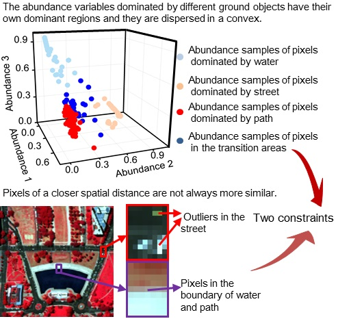
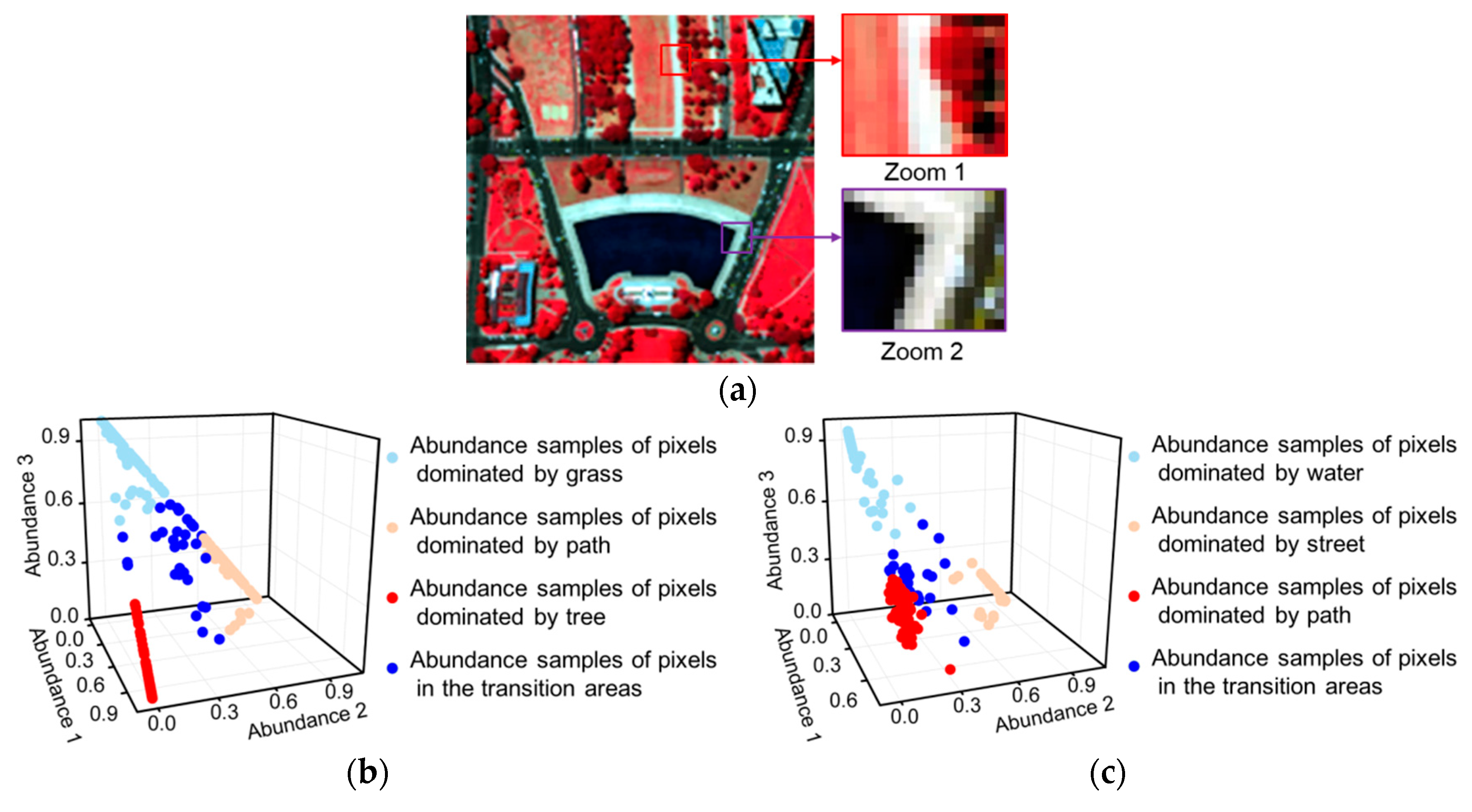
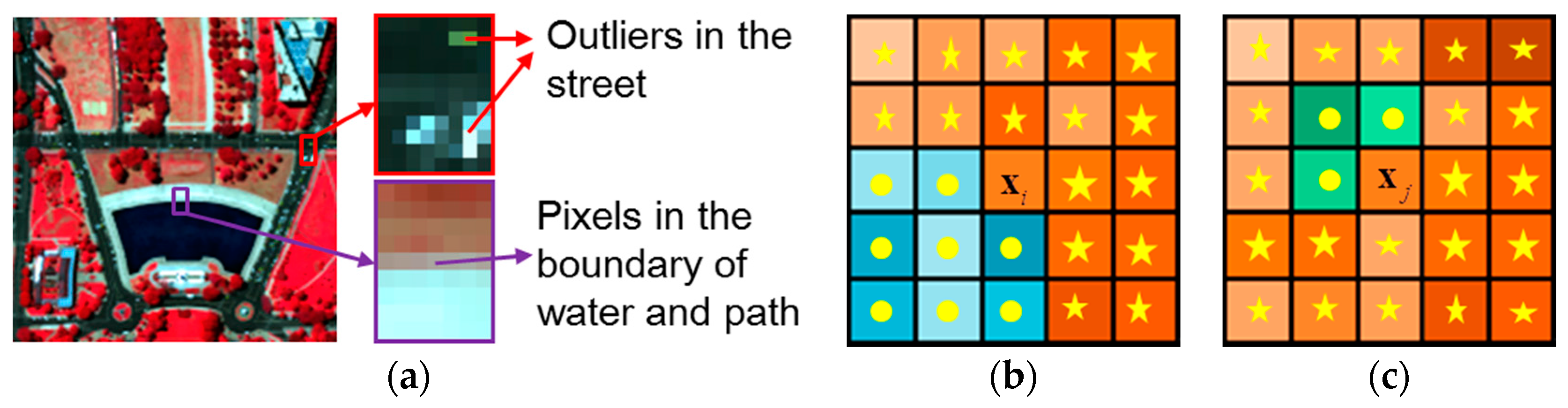
- The smoothness levels of each pixel pair are measured according to the similarities between them by taking advantage of the spectral information of the HSIs. In this way, more similar pixels are given a higher smoothness weight, as shown in Figure 2b,c, which is closer to the reality than a smoothness level determined by spatial distance.
- (2)
- Incorrect smoothness constraints are avoided by assigning a zero smoothness level to the pixels that are dissimilar to the observation pixel. The dissimilar pixels are excluded from the neighborhood pixels in the local window. The schematic diagrams in Figure 2b,c express this idea.
- (3)
- A separation constraint is used to prevent an over-smooth result by utilizing the dispersed characteristic of the abundance variables. A more stable and desirable result can be obtained in the interaction of these two constraints.
2. Related Works
2.1. The Linear Mixing Model (LMM)
2.2. Nonnegative Matrix Factorization (NMF)
3. The Double Abundance Characteristics Constrained NMF Method
3.1. Smoothness Feature of the Abundances
3.2. Dispersed Characteristic of the Abundance Variables
3.3. Abundance Sum-to-One Constraint
3.4. Objective Function and Update Rules of the Proposed Method
3.5. Implementation Issues
3.5.1. Initialization
3.5.2. Stopping Condition
3.5.3. The Procedure of DAC2NMF
- Determine the endmember number P; initialize the endmember matrix by the SID-based algorithm for the synthetic experiments, and VCA algorithm for the real experiments; initialize the abundance matrix according to Equations (28) and (29);
- update by Equation (24);
- replace matrices and with matrices and according to Equation (20);
- update by Equations (25)–(27);
- replace matrices and with matrices and ;
- repeat step 2–step 5 until reaching the maximum number of iterations or Equation (30) is satisfied;
3.5.4. Computational Complexity Analysis
4. Synthetic Image Experiments
4.1. Performance Metrics
4.2. Generation of Synthetic Images
4.3. Performance Evaluation
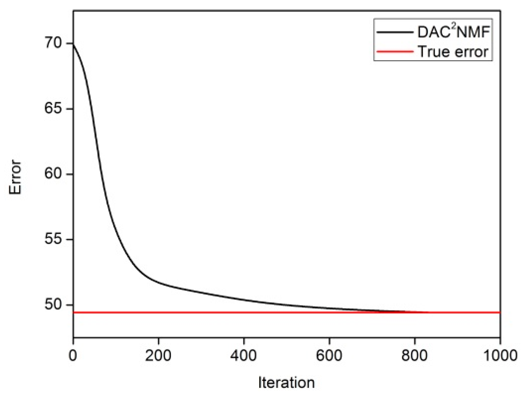
4.3.1. Parameters Selection and Convergence Analysis
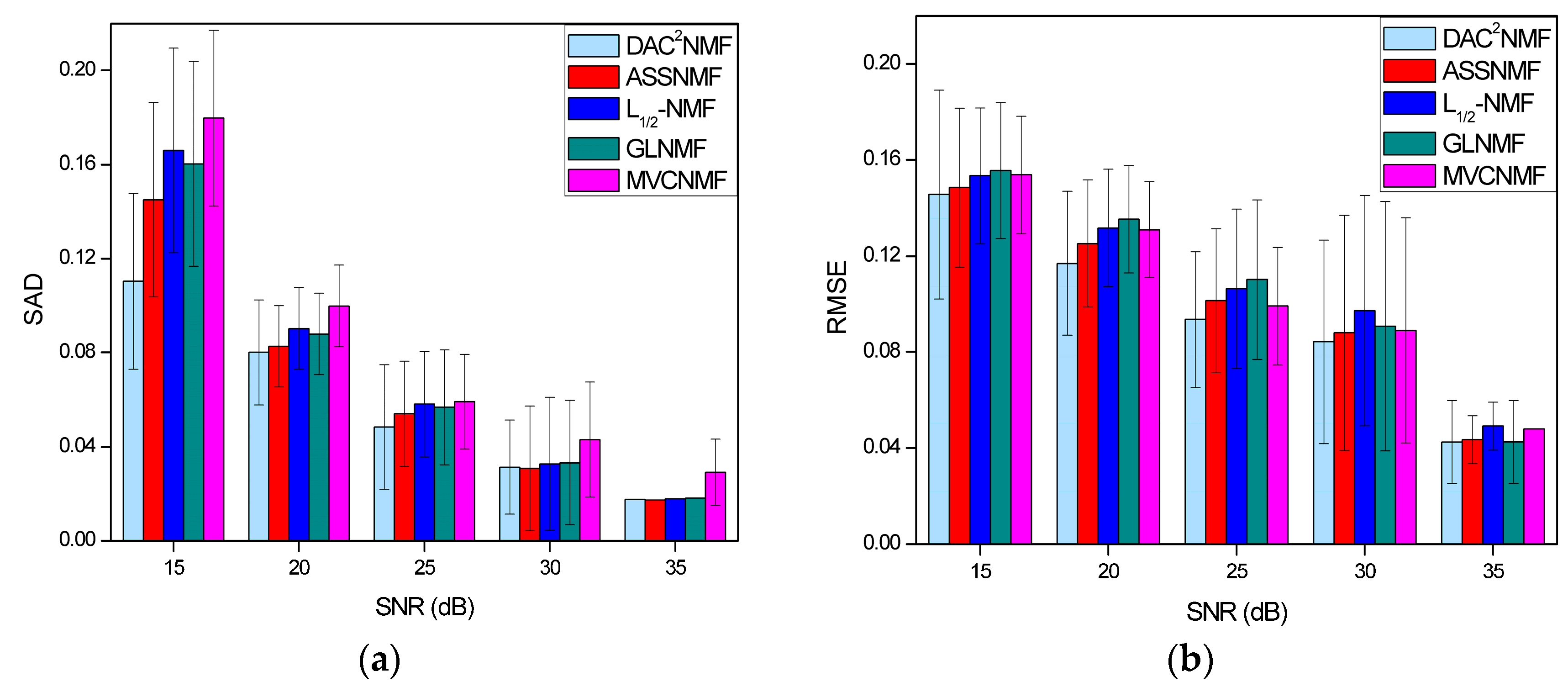
4.3.2. Noise Robustness Analysis
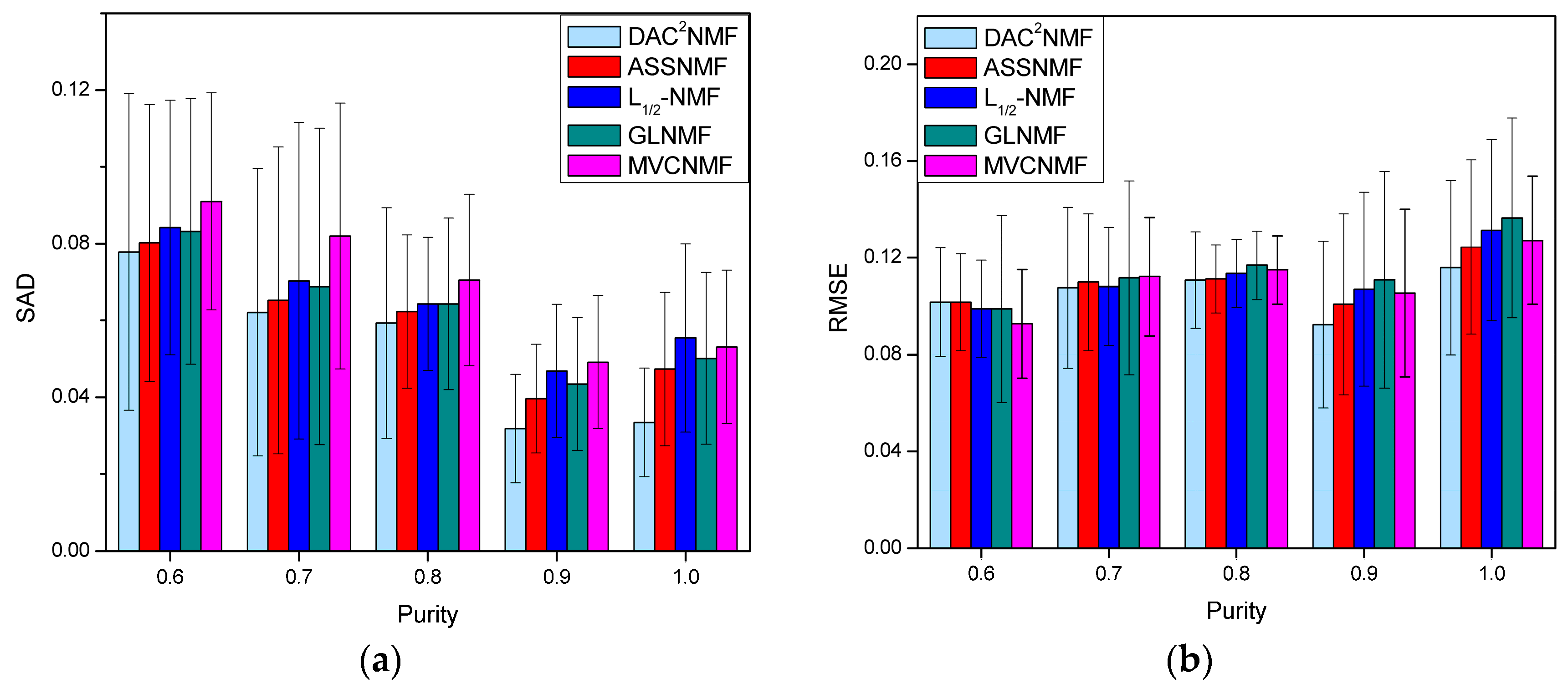
4.3.3. Robustness Analysis to Degree of Mixing
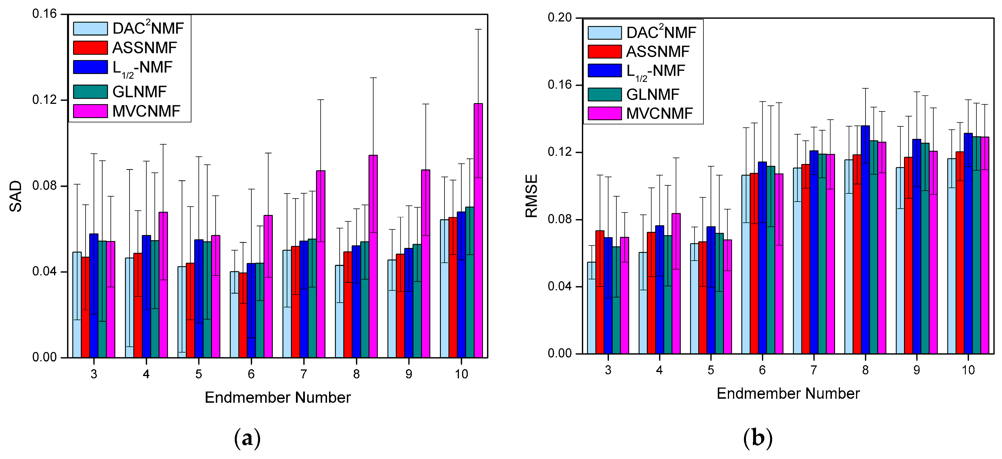
4.3.4. Robustness Analysis to the Number of Endmembers
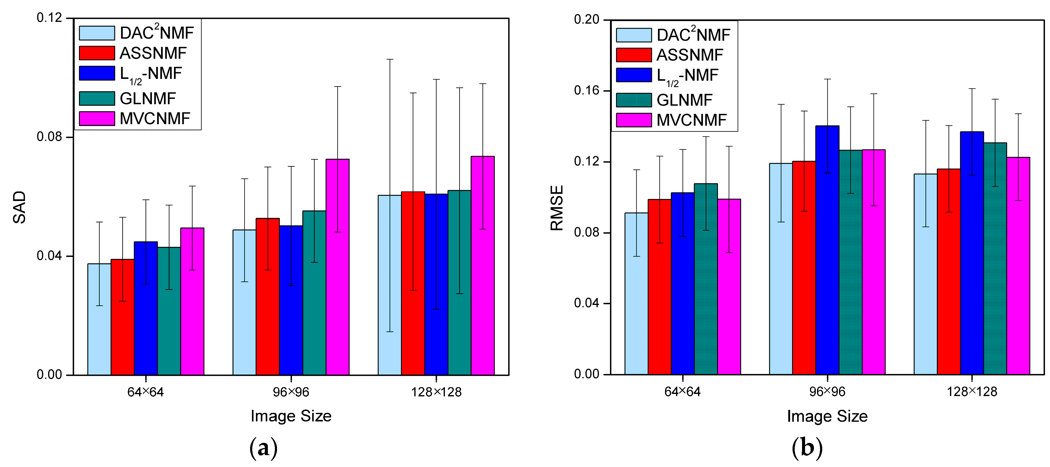
4.3.5. Robustness Analysis to the Image Size
5. Real Data Experiments
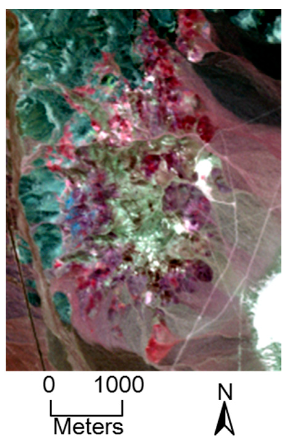
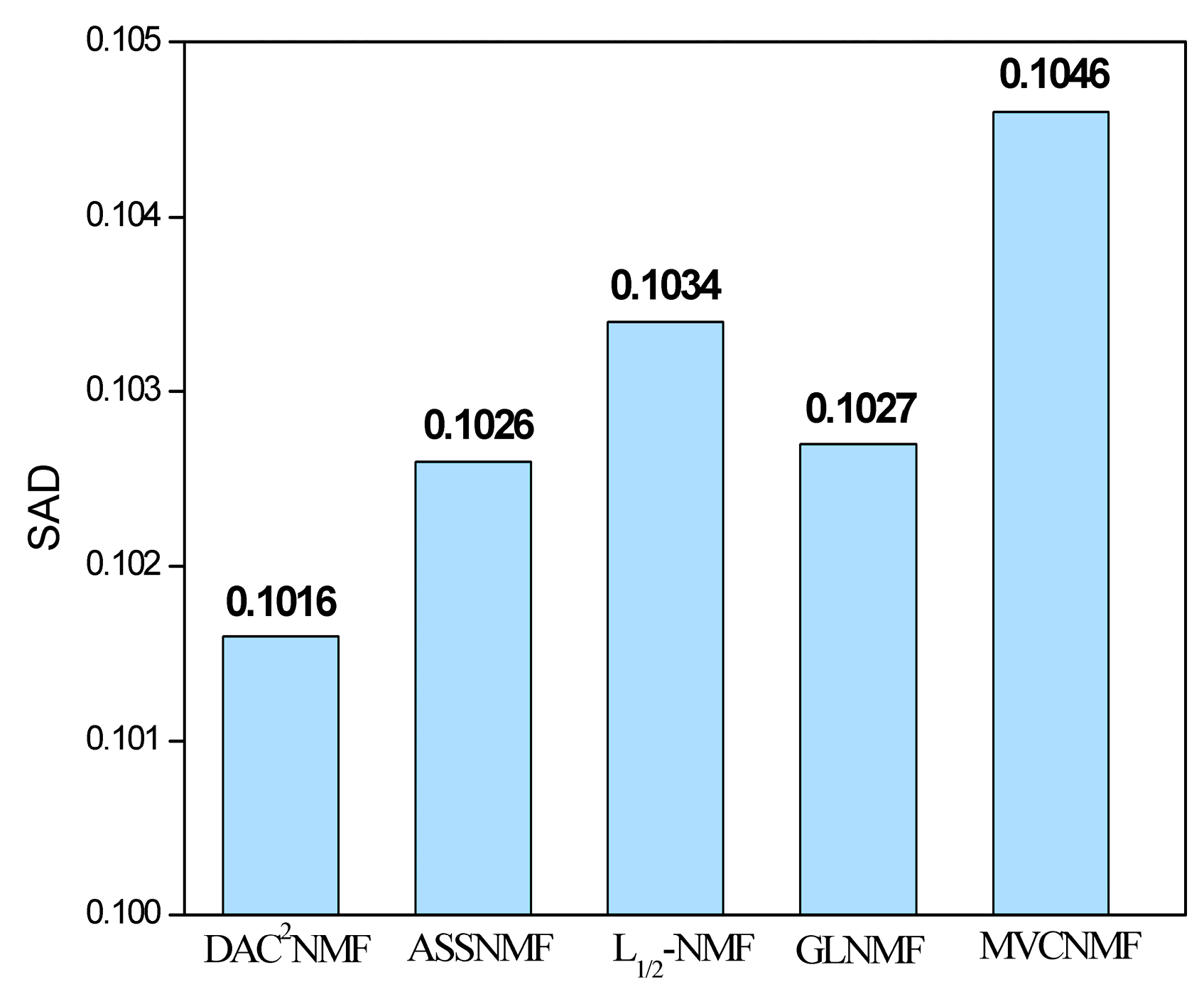
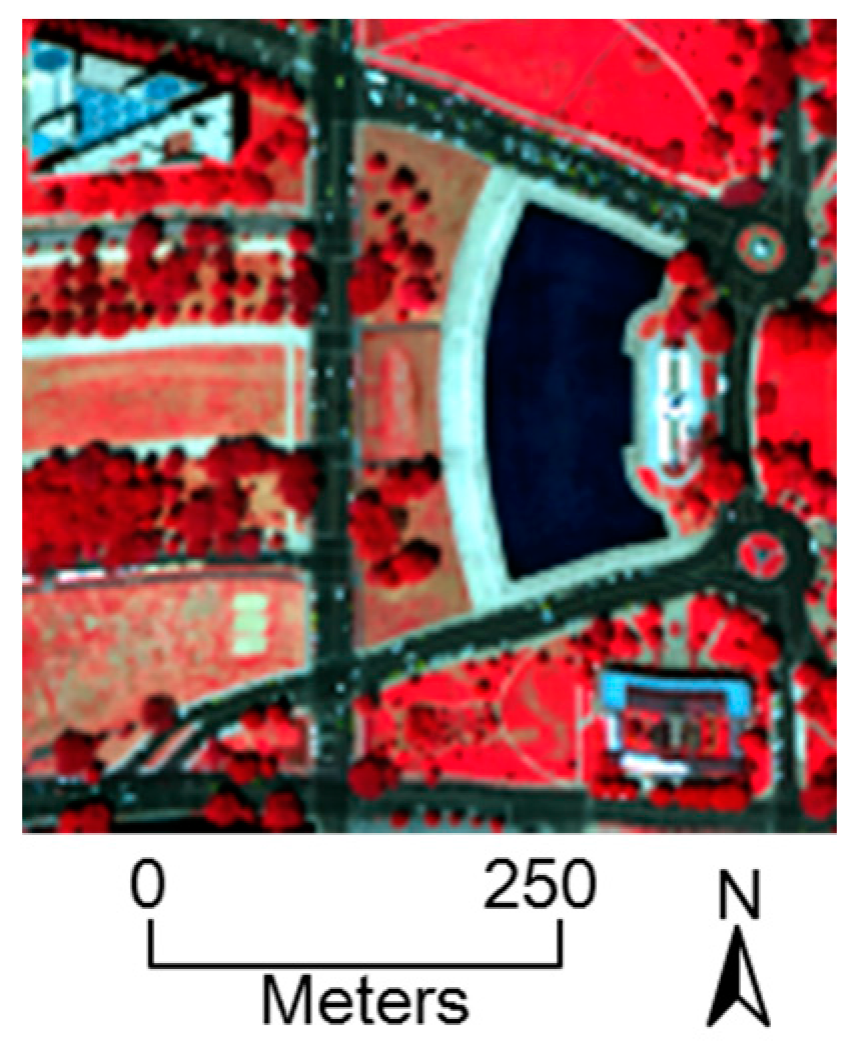
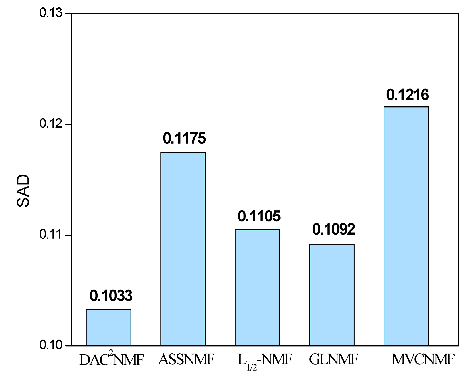
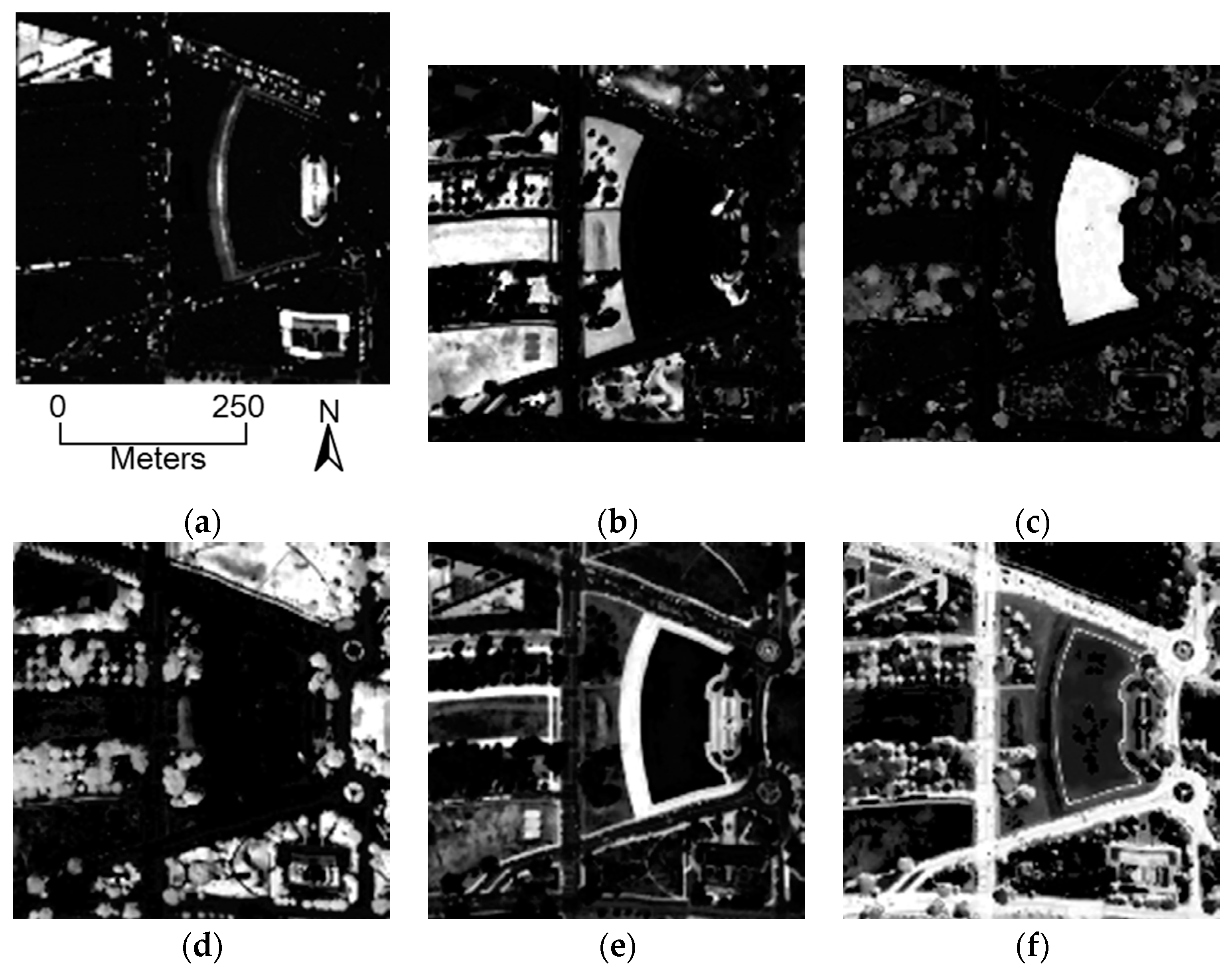
5.1. HYDICE Dataset
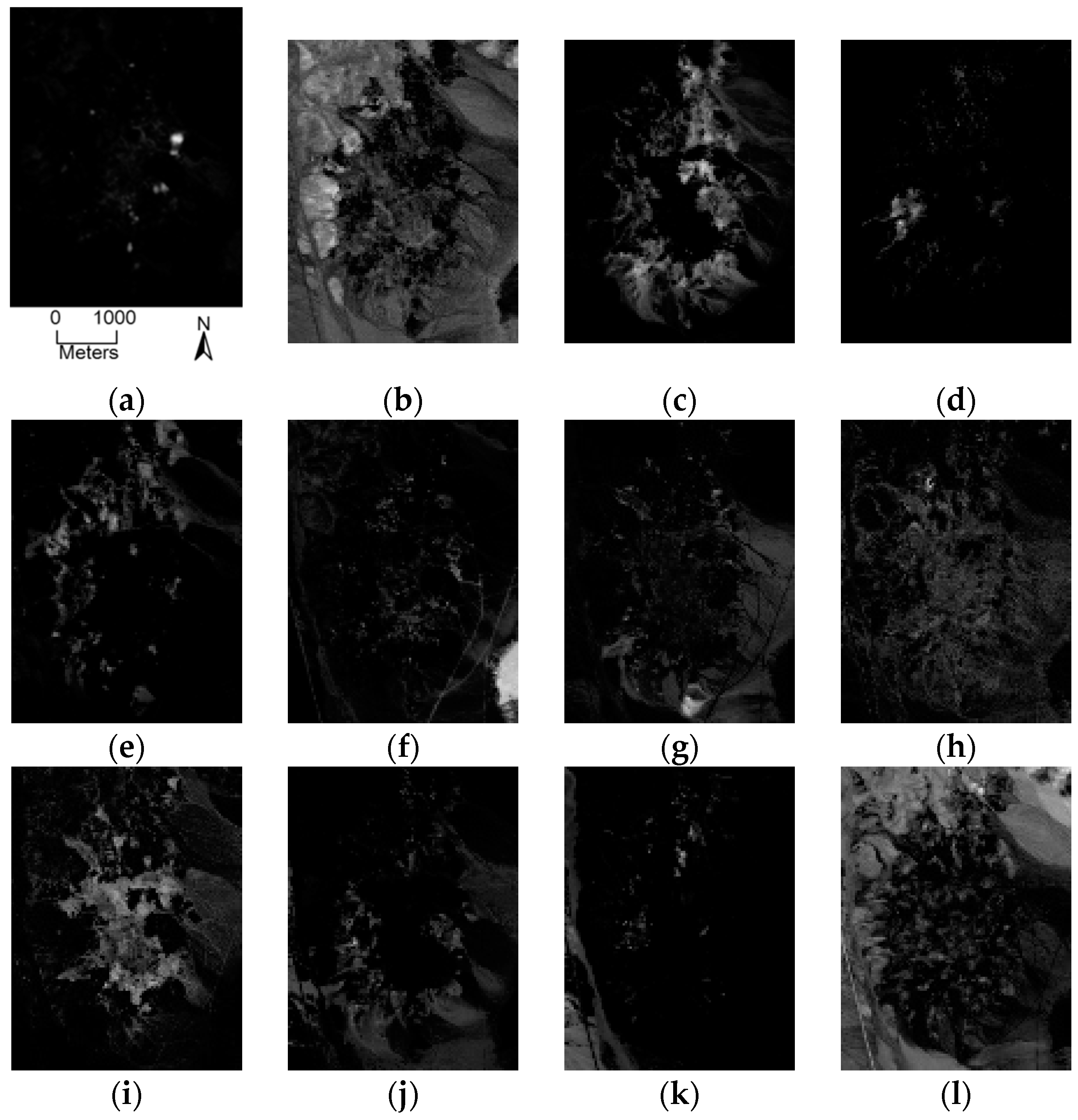
5.2. AVIRIS Dataset
6. Discussion
7. Conclusions
Acknowledgments
Author Contributions
Conflicts of Interest
References
- Tong, Q.; Xue, Y.; Zhang, L. Progress in Hyperspectral Remote Sensing Science and Technology in China Over the Past Three Decades. IEEE J. Sel. Top. Appl. Earth Obs. Remote Sens. 2014, 7, 70–91. [Google Scholar] [CrossRef]
- Bioucas-Dias, J.M.; Plaza, A.; Dobigeon, N.; Parente, M.; Du, Q.; Gader, P.; Chanussot, J. Hyperspectral unmixing overview: Geometrical, statistical, and sparse regression-based approaches. IEEE J. Sel. Top. Appl. Earth Obs. Remote Sens. 2012, 5, 354–379. [Google Scholar] [CrossRef]
- Du, B.; Zhang, L.; Zhang, L.; Chen, T.; Wu, K. A discriminative manifold learning based dimension reduction method for hyperspectral classification. Int. J. Fuzzy Syst. 2012, 14, 272–277. [Google Scholar]
- Keshava, N.; Mustard, J.F. Spectral unmixing. IEEE Signal Process. Mag. 2002, 19, 44–57. [Google Scholar] [CrossRef]
- Parra, L.C.; Spence, C.; Sajda, P.; Ziehe, A.; Müller, K.-R. Unmixing Hyperspectral Data. In Proceedings of the NIPS, Denver, CO, USA, 29 November–4 December 1999; pp. 942–948.
- Roberts, D.A.; Gardner, M.; Church, R.; Ustin, S.; Scheer, G.; Green, R.O. Mapping Chaparral in the Santa Monica Mountains Using Multiple Endmember Spectral Mixture Models. Remote Sens. Environ. 1998, 65, 267–279. [Google Scholar] [CrossRef]
- Zhang, L.; Du, B.; Zhong, Y. Hybrid detectors based on selective endmembers. IEEE Trans. Geosci. Remote Sens. 2010, 48, 2633–2646. [Google Scholar] [CrossRef]
- Bioucas-Dias, J.; Plaza, A.; Camps-Valls, G.; Scheunders, P.; Nasrabadi, N.; Chanussot, J. Hyperspectral remote sensing data analysis and future challenges. IEEE Geosci. Remote Sens. Mag. 2013, 1, 6–36. [Google Scholar] [CrossRef]
- Zhu, F.; Wang, Y.; Fan, B.; Xiang, S.; Meng, G.; Pan, C. Spectral Unmixing via Data-Guided Sparsity. IEEE Trans. Image Process. 2014, 23, 5412–5427. [Google Scholar] [CrossRef] [PubMed]
- Cui, J.; Li, X.; Zhao, L. Linear Mixture Analysis for Hyperspectral Imagery in the Presence of Less Prevalent Materials. IEEE Trans. Geosci. Remote Sens. 2013, 51, 4019–4031. [Google Scholar] [CrossRef]
- Li, J.; Agathos, A.; Zaharie, D.; Bioucas-Dias, J.M.; Plaza, A.; Li, X. Minimum Volume Simplex Analysis: A Fast Algorithm for Linear Hyperspectral Unmixing. IEEE Trans. Geosci. Remote Sens. 2015, 53, 5067–5082. [Google Scholar]
- Boardman, J.W. Automating spectral unmixing of AVIRIS data using convex geometry concepts. In Proceedings of the Summaries 4th Annu. JPL Airborne Geoscience Workshop, Washington, DC, USA, 25–29 October 1993; Volume 1, pp. 11–14.
- Winter, M.E. N-FINDR: An algorithm for fast autonomous spectral end-member determination in hyperspectral data. Proc. SPIE 1999, 3753. [Google Scholar] [CrossRef]
- Chang, C.-I.; Wu, C.-C.; Liu, W.-M.; Ouyang, Y.-C. A new growing method for simplex-based endmember extraction algorithm. IEEE Trans. Geosci. Remote Sens. 2006, 44, 2804–2819. [Google Scholar] [CrossRef]
- Nascimento, J.M.; Dias, J.M.B. Vertex component analysis: A fast algorithm to unmix hyperspectral data. IEEE Trans. Geosci. Remote Sens. 2005, 43, 898–910. [Google Scholar] [CrossRef]
- Chan, T.-H.; Chi, C.-Y.; Huang, Y.-M.; Ma, W.-K. A convex analysis-based minimum-volume enclosing simplex algorithm for hyperspectral unmixing. IEEE Trans. Signal Process. 2009, 57, 4418–4432. [Google Scholar] [CrossRef]
- Bioucas-Dias, J.M. A variable splitting augmented Lagrangian approach to linear spectral unmixing. In Proceedings of the IEEE GRSS Workshop Hyperspectral Image Signal Processing: Evolution in Remote Sensing (WHISPERS), Grenoble, France, 26–28 August 2009; pp. 1–4.
- Iordache, M.D.; Bioucas-Dias, J.M.; Plaza, A. Sparse Unmixing of Hyperspectral Data. IEEE Trans. Geosci. Remote Sens. 2011, 49, 2014–2039. [Google Scholar] [CrossRef]
- Ma, W.; Bioucas-Dias, J.; Chan, T.; Gillis, N.; Gader, P.; Plaza, A.; Ambikapathi, A.; Chi, C.-Y. A signal processing perspective on hyperspectral unmixing: Insights from remote sensing. IEEE Signal Process. Mag. 2014, 31, 67–81. [Google Scholar] [CrossRef]
- Bioucas-Dias, J.M.; Figueiredo, M.A. Alternating direction algorithms for constrained sparse regression: Application to hyperspectral unmixing. In Proceedings of the IEEE GRSS Workshop Hyperspectral Image Signal Processing: Evolution in Remote Sensing (WHISPERS), Reykjavik, Icelane, 14–16 June 2010; pp. 1–4.
- Iordache, M.-D.; Bioucas-Dias, J.M.; Plaza, A. Total variation spatial regularization for sparse hyperspectral unmixing. IEEE Trans. Geosci. Remote Sens. 2012, 50, 4484–4502. [Google Scholar] [CrossRef]
- Iordache, M.-D.; Bioucas-Dias, J.M.; Plaza, A. Collaborative sparse regression for hyperspectral unmixing. IEEE Trans. Geosci. Remote Sens. 2014, 52, 341–354. [Google Scholar] [CrossRef]
- Qu, Q.; Nasrabadi, N.M.; Tran, T.D. Abundance Estimation for Bilinear Mixture Models via Joint Sparse and Low-Rank Representation. IEEE Trans. Geosci. Remote Sens. 2014, 52, 4404–4423. [Google Scholar]
- Giampouras, P.V.; Themelis, K.E.; Rontogiannis, A.A.; Koutroumbas, K.D. Simultaneously Sparse and Low-Rank Abundance Matrix Estimation for Hyperspectral Image Unmixing. IEEE Trans. Geosci. Remote Sens. 2016, PP, 1–15. [Google Scholar] [CrossRef]
- Hyvärinen, A.; Oja, E. Independent component analysis: Algorithms and applications. Neural Netw. 2000, 13, 411–430. [Google Scholar] [CrossRef]
- Lee, D.D.; Seung, H.S. Algorithms for non-negative matrix factorization. In Proceedings of the NIPS 2000, Breckenridge, CO, USA, 2 December 2000; pp. 556–562.
- Nascimento, J.M.; Dias, J.M. Does independent component analysis play a role in unmixing hyperspectral data? IEEE Trans. Geosci. Remote Sens. 2005, 43, 175–187. [Google Scholar] [CrossRef]
- Nascimento, J.M.; Bioucas-Dias, J.M. Hyperspectral unmixing based on mixtures of Dirichlet components. IEEE Trans. Geosci. Remote Sens. 2012, 50, 863–878. [Google Scholar] [CrossRef]
- Xia, W.; Liu, X.; Wang, B.; Zhang, L. Independent component analysis for blind unmixing of hyperspectral imagery with additional constraints. IEEE Trans. Geosci. Remote Sens. 2011, 49, 2165–2179. [Google Scholar] [CrossRef]
- Wang, N.; Du, B.; Liangpei, Z.; Zhang, L. An Abundance Characteristic-Based Independent Component Analysis for Hyperspectral Unmixing. IEEE Trans. Geosci. Remote Sens. 2015, 53, 416–428. [Google Scholar] [CrossRef]
- Yang, Z.; Guoxu, Z.; Xie, S.; Ding, S.; Yang, J.-M.; Zhang, J. Blind Spectral Unmixing Based on Sparse Nonnegative Matrix Factorization. IEEE Trans. Image Process. 2011, 20, 1112–1125. [Google Scholar] [CrossRef] [PubMed]
- Jia, S.; Qian, Y. Constrained nonnegative matrix factorization for hyperspectral unmixing. IEEE Trans. Geosci. Remote Sens. 2009, 47, 161–173. [Google Scholar] [CrossRef]
- Miao, L.; Qi, H. Endmember extraction from highly mixed data using minimum volume constrained nonnegative matrix factorization. IEEE Trans. Geosci. Remote Sens. 2007, 45, 765–777. [Google Scholar] [CrossRef]
- Wang, N.; Du, B.; Zhang, L. An Endmember Dissimilarity Constrained Non-Negative Matrix Factorization Method for Hyperspectral Unmixing. IEEE J. Sel. Top. Appl. Earth Obs. Remote Sens. 2013, 6, 554–569. [Google Scholar] [CrossRef]
- Liu, X.; Xia, W.; Wang, B.; Zhang, L. An approach based on constrained nonnegative matrix factorization to unmix hyperspectral data. IEEE Trans. Geosci. Remote Sens. 2011, 49, 757–772. [Google Scholar] [CrossRef]
- Qian, Y.; Jia, S.; Zhou, J.; Robles-Kelly, A. Hyperspectral Unmixing via L1/2 Sparsity-Constrained Nonnegative Matrix Factorization. IEEE Trans. Geosci. Remote Sens. 2011, 49, 4282–4297. [Google Scholar] [CrossRef]
- Sigurdsson, J.; Ulfarsson, M.O.; Sveinsson, J.R. Hyperspectral Unmixing With lq Regularization. IEEE Trans. Geosci. Remote Sens. 2014, 52, 6793–6806. [Google Scholar] [CrossRef]
- He, W.; Zhang, H.; Zhang, L. Sparsity-Regularized Robust Non-Negative Matrix Factorization for Hyperspectral Unmixing. IEEE J. Sel. Top. Appl. Earth Obs. Remote Sens. 2016, PP, 1–13. [Google Scholar] [CrossRef]
- Liu, J.; Zhang, J.; Gao, Y.; Zhang, C.; Li, Z. Enhancing Spectral Unmixing by Local Neighborhood Weights. IEEE J. Sel. Top. Appl. Earth Obs. Remote Sens. 2012, 5, 1545–1552. [Google Scholar]
- Martin, G.; Plaza, A. Spatial-Spectral Preprocessing Prior to Endmember Identification and Unmixing of Remotely Sensed Hyperspectral Data. IEEE J. Sel. Top. Appl. Earth Obs. Remote Sens. 2012, 5, 380–395. [Google Scholar] [CrossRef]
- Yuan, Y.; Min, F.; Xiaoqiang, L. Substance Dependence Constrained Sparse NMF for Hyperspectral Unmixing. IEEE Trans. Geosci. Remote Sens. 2015, 53, 2975–2986. [Google Scholar] [CrossRef]
- Lu, X.; Wu, H.; Yuan, Y.; Yan, P.; Li, X. Manifold regularized sparse NMF for hyperspectral unmixing. IEEE Trans. Geosci. Remote Sens. 2013, 51, 2815–2826. [Google Scholar] [CrossRef]
- Lee, D.D.; Seung, H.S. Learning the parts of objects by non-negative matrix factorization. Nature 1999, 401, 788–791. [Google Scholar] [PubMed]
- Huang, S.; Elhoseiny, M.; Elgammal, A.; Yang, D. Improving non-negative matrix factorization via ranking its bases. In Proceedings of the 2014 IEEE International Conference on Image Processing (ICIP), Paris, France, 27–30 October 2014; pp. 5951–5955.
- Li, L.; Yang, J.; Xu, Y.; Qin, Z.; Zhang, H. Documents clustering based on max-correntropy nonnegative matrix factorization. In Proceedings of the 2014 International Conference on Machine Learning and Cybernetics (ICMLC), Lanzhou, China, 13–16 July 2014; pp. 850–855.
- Chang, C.-I. An information-theoretic approach to spectral variability, similarity, and discrimination for hyperspectral image analysis. IEEE Trans. Inf. Theory. 2000, 46, 1927–1932. [Google Scholar] [CrossRef]
- Dennison, P.E.; Halligan, K.Q.; Roberts, D.A. A comparison of error metrics and constraints for multiple endmember spectral mixture analysis and spectral angle mapper. Remote Sens. Environ. 2004, 93, 359–367. [Google Scholar] [CrossRef]
- Zelnik-manor, L.; Perona, P. Self-tuning spectral clustering. In Proceedings of the Advances in Neural Information Processing Systems, Vancouver, BC, Canada, 13–18 December 2004; pp. 1601–1608.
- Chen, C.H.; Zhang, X. Independent component analysis for remote sensing study. Proc. SPIE 1999, 3871. [Google Scholar] [CrossRef]
- Heinz, D.C.; Chang, C.-I. Fully constrained least squares linear spectral mixture analysis method for material quantification in hyperspectral imagery. IEEE Trans. Geosci. Remote Sens. 2001, 39, 529–545. [Google Scholar] [CrossRef]
- Chang, C.-I.; Du, Q. Estimation of number of spectrally distinct signal sources in hyperspectral imagery. IEEE Trans. Geosci. Remote Sens. 2004, 42, 608–619. [Google Scholar] [CrossRef]
- Bioucas-Dias, J.M.; Nascimento, J.M. Hyperspectral subspace identification. IEEE Trans. Geosci. Remote Sens. 2008, 46, 2435–2445. [Google Scholar] [CrossRef]
- Wang, S.; Wang, N.; Tao, D.; Zhang, L.; Du, B. A K-L divergence constrained sparse NMF for hyperspectral signal unmixing. In Proceedings of the International Conference on Security, Pattern Analysis, and Cybernetics (SPAC), Wuhan, China, 18–19 October 2014; pp. 223–228.
- Rogge, D.; Rivard, B.; Zhang, J.; Sanchez, A.; Harris, J.; Feng, J. Integration of spatial–spectral information for the improved extraction of endmembers. Remote Sens. Environ. 2007, 110, 287–303. [Google Scholar] [CrossRef]


| Algorithms | Computational Complexity |
|---|---|
| DAC2NMF | |
| ASSNMF | |
| GLNMF | |
| MVCNMF |
| DAC2NMF | ASSNMF | GLNMF | MVCNMF | ||
|---|---|---|---|---|---|
| Roof | 0.0458 | 0.0904 | 0.0846 | 0.0946 | 0.0613 |
| Grass | 0.2153 | 0.214 | 0.2246 | 0.2209 | 0.2803 |
| Water | 0.1082 | 0.145 | 0.1372 | 0.1378 | 0.1464 |
| Tree | 0.0223 | 0.0327 | 0.0325 | 0.0239 | 0.076 |
| Path | 0.1398 | 0.1437 | 0.1323 | 0.1302 | 0.1079 |
| Street | 0.0882 | 0.079 | 0.0518 | 0.0477 | 0.0576 |
| DAC2NMF | ASSNMF | GLNMF | MVCNMF | ||
|---|---|---|---|---|---|
| Muscovite | 0.0663 | 0.0674 | 0.069 | 0.0684 | 0.0685 |
| Sphene | 0.0523 | 0.0508 | 0.0538 | 0.0527 | 0.0581 |
| Alunite | 0.0905 | 0.0909 | 0.0996 | 0.09 | 0.1067 |
| Buddingtonite | 0.1087 | 0.1032 | 0.1032 | 0.1016 | 0.1012 |
| Nontronite#1 | 0.1018 | 0.1052 | 0.1072 | 0.104 | 0.1023 |
| Montmorillonite#1 | 0.0794 | 0.082 | 0.0829 | 0.0831 | 0.0833 |
| Dumortierite | 0.0761 | 0.0781 | 0.0785 | 0.0755 | 0.0768 |
| Nontronite#2 | 0.0715 | 0.0684 | 0.0692 | 0.0694 | 0.0713 |
| Chalcedony | 0.1231 | 0.1257 | 0.1257 | 0.1233 | 0.1212 |
| Kaolinite#1 | 0.1828 | 0.1857 | 0.1823 | 0.1866 | 0.187 |
| Kaolinite#2 | 0.2218 | 0.2257 | 0.2209 | 0.2273 | 0.2278 |
| Montmorillonite#2 | 0.0454 | 0.0476 | 0.048 | 0.05 | 0.0508 |
© 2016 by the authors; licensee MDPI, Basel, Switzerland. This article is an open access article distributed under the terms and conditions of the Creative Commons Attribution (CC-BY) license (http://creativecommons.org/licenses/by/4.0/).
Share and Cite
Liu, R.; Du, B.; Zhang, L. Hyperspectral Unmixing via Double Abundance Characteristics Constraints Based NMF. Remote Sens. 2016, 8, 464. https://doi.org/10.3390/rs8060464
Liu R, Du B, Zhang L. Hyperspectral Unmixing via Double Abundance Characteristics Constraints Based NMF. Remote Sensing. 2016; 8(6):464. https://doi.org/10.3390/rs8060464
Chicago/Turabian StyleLiu, Rong, Bo Du, and Liangpei Zhang. 2016. "Hyperspectral Unmixing via Double Abundance Characteristics Constraints Based NMF" Remote Sensing 8, no. 6: 464. https://doi.org/10.3390/rs8060464