
Relating the Age of Arctic Sea Ice to its Thickness, as Measured during NASA’s ICESat and IceBridge Campaigns


Abstract
:
1. Introduction
2. Materials and Methods
2.1. Ice Age Product
2.2. Thickness Data Sets
2.3. Method
2.3.1. ICESat
2.3.2. IceBridge
3. Results
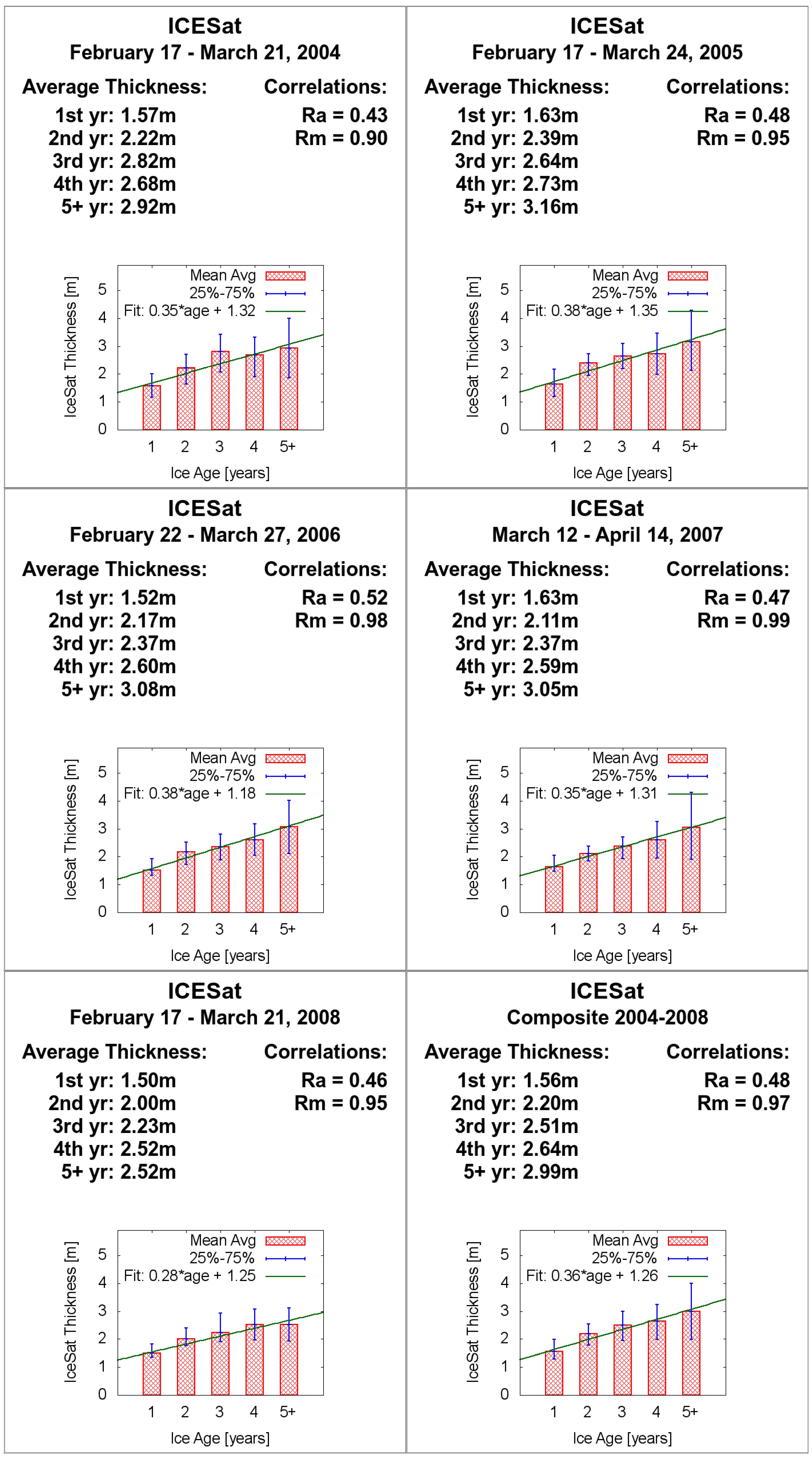
3.1. ICESat
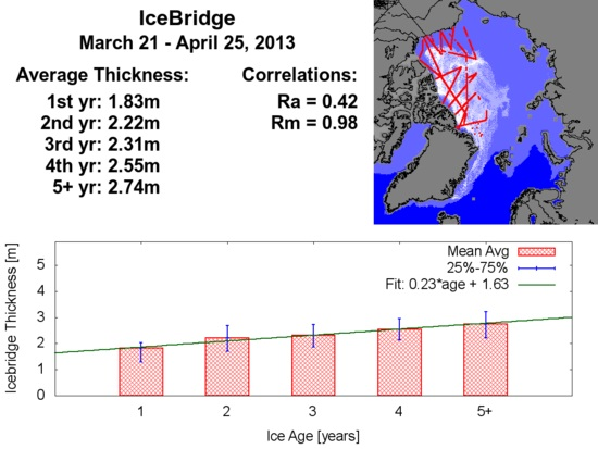
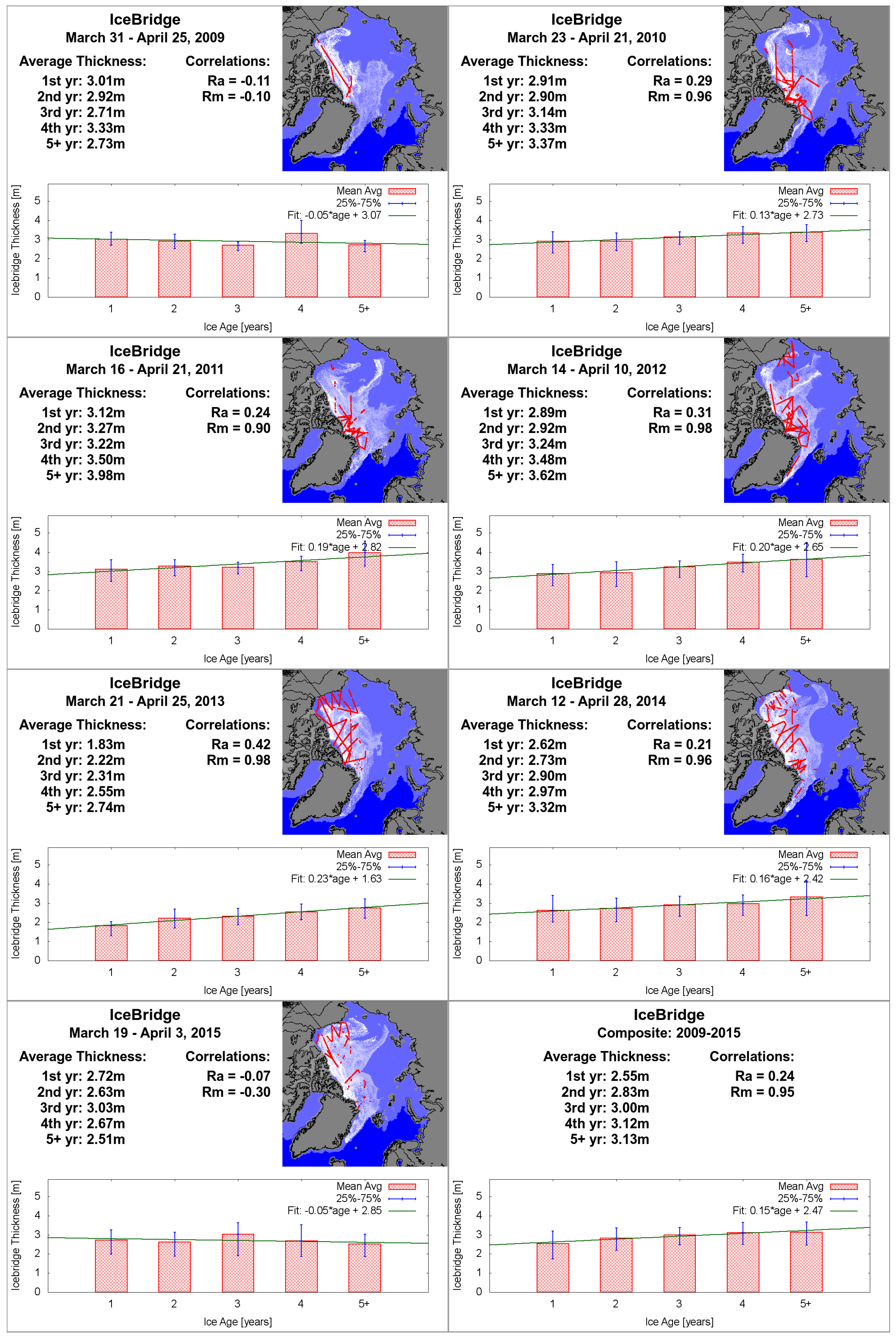
3.2. IceBridge
4. Discussion
5. Conclusions
Acknowledgments
Author Contribution
Conflicts of Interest
Abbreviations
| AMSR-E | Advanced Microwave Scanning Radiometer - Earth Observing System |
| CICE | The Los Alamos sea ice model |
| EASE | Equal Area Scalable Earth grid |
| FYI | First-year ice |
| ICESat | Ice, Cloud, and land Elevation Satellite |
| IABP | International Arctic Buoy Program |
| LIDAR | Light Detection and Ranging |
| MYI | Multi-year ice |
| NCAR | National Center for Atmospheric Research |
| NCEP | National Centers for Environmental Prediction |
| NSIDC | National Snow and Ice Data Center |
| Ra | Correlation coefficient using all ice thickness data points |
| Rm | Correlation coefficient using only mean ice thickness data points for each ice age class |
| RADAR | RAdio Detection And Ranging |
| RMS | root-mean-square |
| SMMR | Scanning Multichannel Microwave Radiometer |
| SSM/I | Special Sensor Microwave Imager |
| SSMIS | SSM/I Sounder |
References
- Serreze, M.C.; Holland, M.M.; Stroeve, J. Perspectives on the Arctic’s shrinking sea-ice cover. Science 2007, 315, 1533–1536. [Google Scholar] [CrossRef] [PubMed]
- Stroeve, J.C.; Serreze, M.C.; Holland, M.M.; Kay, J.E.; Maslanik, J.; Barrett, A.P. The Arctic’s rapidly shrinking sea ice cover: A research synthesis. Clim. Chang. 2012, 110, 1005–1027. [Google Scholar] [CrossRef]
- Serreze, M.C.; Stroeve, J. Arctic sea ice trends, variability and implications for seasonal ice forecasting. Phil. Trans. R. Soc. A 2015, 373. [Google Scholar] [CrossRef] [PubMed]
- Kwok, R.; Rothrock, D.A. Decline in Arctic sea ice thickness from submarine and ICESat records. Geophys. Res. Lett. 2009, 36. [Google Scholar] [CrossRef]
- Maslanik, J.A.; Stroeve, J.; Fowler, C.; Emery, W. Distribution and trends in Arctic sea ice age through spring 2011. Geophys. Res. Lett. 2011, 38. [Google Scholar] [CrossRef]
- Maslanik, J.A.; Fowler, C.; Stroeve, J.; Drobot, S.; Zwally, J.; Yi, D.; Emery, W. A younger, thinner Arctic ice cover: Increased potential for rapid, extensive sea-ice loss. Geophys. Res. Lett. 2007, 34, L24501. [Google Scholar] [CrossRef]
- Nghiem, S.V.; Rigor, G.; Perovich, D.K.; Clemente-Colón, P.; Weatherly, J.W.; Neumann, G. Rapid reduction of Arctic perennial sea ice. Geophys. Res. Lett. 2006, 34. [Google Scholar] [CrossRef]
- Kwok, R.; Cunningham, G.F. ICESat over Arctic sea ice: Estimation of snow depth and ice thickness. J. Geophys. Res. 2008, 113. [Google Scholar] [CrossRef]
- Tschudi, M.; Fowler, C.; Maslanik, J. EASE-Grid Sea Ice Age, Version 2; NASA National Snow and Ice Data Center Distributed Active Archive Center: Boulder, CO, USA, 2015; Available online: http://dx.doi.org/10.5067/1UQJWCYPVX61 (accessed on 1 November 2015).
- Holland, M.M.; Bitz, C.M.; Tremblay, B. Future abrupt reductions in the summer Arctic sea ice. Geophys. Res. Lett. 2006, 33. [Google Scholar] [CrossRef]
- Kwok, R.; Zwally, H.J.; Yi, D. ICESat observations of Arctic sea ice: A first look. Geophys. Res. Lett. 2004, 31. [Google Scholar] [CrossRef]
- Bitz, C.M.; Holland, M.M.; Weaver, A.J.; Eby, M. Simulating the ice-thickness distribution in a coupled climate model. J. Geophys. Res. 2001, 106, 2441–2463. [Google Scholar] [CrossRef]
- Perovich, D.K.; Richter-Menge, J.A.; Jones, K.F.; Light, B. Sunlight, water, and ice: Extreme Arctic sea ice melt during the summer of 2007. Geophys. Res. Lett. 2008, 35. [Google Scholar] [CrossRef]
- Studinger, M.; Koenig, L.; Martin, S.; Sonntag, J. Operation icebridge: Using instrumented aircraft to bridge the observational gap between Icesat and Icesat-2. In Proceedings of the 2010 IEEE International Geoscience and Remote Sensing Symposium, Honolulu, HI, USA, 25–30 July2010; pp. 1918–1919.
- Meier, W.N.; Maslanik, J.A.; Fowler, C.W. Error analysis and assimilation of remotely sensed ice motion within an Arctic sea ice model. J. Geophys. Res. 2000, 105, 3339–3356. [Google Scholar] [CrossRef]
- Fowler, C.; Maslanik, J.; Emery, W.; Tschudi, M. Polar Pathfinder Daily 25 km EASE-Grid Sea Ice Motion Vectors, Version 2; National Snow and Ice Data Center: Boulder, CO, USA, 2013. [Google Scholar]
- Cavalieri, D.J.; Gloersen, P.; Campbell, W.J. Determination of sea ice parameters with the NIMBUS 7 scanning multichannel microwave radiometer. J. Geophys. Res. 1984, 89, 5355–5369. [Google Scholar] [CrossRef]
- Comiso, J.C. A rapidly declining perennial sea ice cover in the Arctic. Geophys. Res. Lett. 2002, 29. [Google Scholar] [CrossRef]
- Rigor, I.G.; Wallace, J.M. Variations in the age of Arctic sea-ice and summer sea-ice extent. Geophys. Res. Lett. 2004, 31. [Google Scholar] [CrossRef]
- Sumata, H.; Kwok, R.; Gerdes, R.; Kauker, F.; Karcher, M. Uncertainty of Arctic summer ice drift assessed by high-resolution SAR data. J. Geophys. Res. Oceans. 2015. [Google Scholar] [CrossRef]
- Tschudi, M.A.; Fowler, C.; Maslanik, J.A.; Stroeve, J. Tracking the movement and changing surface characteristics of Arctic sea ice. IEEE J. Sel. Top. Earth Obs. Remote Sens. 2010. [Google Scholar] [CrossRef]
- Kurtz, N.; Farrell, S.L.; Studinger, M.; Galin, N.; Harbeck, J.P.; Lindsay, R.; Onana, V.D.; Panzer, B.; Sonntag, J.G. Sea ice thickness, freeboard, and snow depth products from operation IceBridge airborne data. Cryosphere 2012, 6, 4771–4827. [Google Scholar] [CrossRef]
- Kurtz, N.; Studinger, M.S.; Harbeck, J.; Onana, V.; Yi, D. IceBridge L4 Sea Ice Freeboard, Snow Depth, and Thickness, Version 1; NASA National Snow and Ice Data Center Distributed Active Archive Center: Boulder, CO, USA, 2015. [Google Scholar]
- Zygmuntowska, M.; Rampal, P.; Ivanova, N.; Smedsrud, L.H. Uncertainties in Arctic sea ice thickness and volume: New estimates and implications for trends. Cryosphere 2014, 8, 705–720. [Google Scholar] [CrossRef]
- Kwok, R. ICESat: Sea Ice Thickness and Freeboard. Available online: http://rkwok.jpl.nasa.gov/icesat/download.html (accessed on 12 December 2015).
- NSIDC. Available online: https://nsidc.org/data/docs/daac/icebridge/evaluation_products/sea-ice-freeboard-snowdepth-thickness-quicklook-index.html (accessed on 17 October 2015).
- NSIDC. March 2009–2015: Arctic Sea Ice News and Analysis. Available online: https://nsidc.org/arcticseaicenews/ (accessed on 23 February 2016).
- Tilling, R.L.; Ridout, A.; Shepherd, A.; Wingham, D.J. Increased Arctic sea ice volume after anomalously low melting in 2013. Nat. Geosci. 2015, 8, 643–646. [Google Scholar] [CrossRef]
- Galley, R.; Hwang, B.J.; Barber, D.; Key, E.; Ehn, J.K. Spatial and temporal variability of sea ice in the CASES study region: 1980–2004. J. Geophys. Res. 2008, 113. [Google Scholar] [CrossRef]
- Perovich, D.; Meier, W.; Tschudi, M.; Farrell, S.; Gerland, S.; Hendricks, S. Arctic Report Card: Update for 2015, Sea Ice. Available online: http://www.arctic.noaa.gov/reportcard/sea_ice.html (accessed on 24 February 2016).
- Laxon, S.W.; Giles, K.A.; Ridout, A.L.; Wingham, D.J.; Willatt, R.; Cullen, R.; Kwok, R.; Schweiger, A.; Zhang, J.; Haas, C.; et al. CryoSat-2 estimates of Arctic sea ice thickness and volume. Geophys. Res. Lett. 2013, 40. [Google Scholar] [CrossRef]


| Year | 1st-year | 2nd-year | 3rd-year | 4th-year | 5th-year+ | Total | Mean Ice Thickness (m) |
|---|---|---|---|---|---|---|---|
| 2009 | 23 | 22 | 32 | 34 | 117 | 228 | 2.86 |
| 2010 | 184 | 201 | 163 | 73 | 243 | 864 | 3.12 |
| 2011 | 97 | 179 | 252 | 74 | 89 | 691 | 3.35 |
| 2012 | 373 | 218 | 310 | 279 | 39 | 1219 | 3.03 |
| 2013 | 396 | 141 | 189 | 148 | 144 | 1018 | 2.21 |
| 2014 | 154 | 207 | 169 | 185 | 146 | 861 | 2.24 |
| 2015 | 85 | 60 | 72 | 82 | 124 | 423 | 2.69 |
© 2016 by the authors; licensee MDPI, Basel, Switzerland. This article is an open access article distributed under the terms and conditions of the Creative Commons Attribution (CC-BY) license (http://creativecommons.org/licenses/by/4.0/).
Share and Cite
Tschudi, M.A.; Stroeve, J.C.; Stewart, J.S. Relating the Age of Arctic Sea Ice to its Thickness, as Measured during NASA’s ICESat and IceBridge Campaigns. Remote Sens. 2016, 8, 457. https://doi.org/10.3390/rs8060457
Tschudi MA, Stroeve JC, Stewart JS. Relating the Age of Arctic Sea Ice to its Thickness, as Measured during NASA’s ICESat and IceBridge Campaigns. Remote Sensing. 2016; 8(6):457. https://doi.org/10.3390/rs8060457
Chicago/Turabian StyleTschudi, Mark A., Julienne C. Stroeve, and J. Scott Stewart. 2016. "Relating the Age of Arctic Sea Ice to its Thickness, as Measured during NASA’s ICESat and IceBridge Campaigns" Remote Sensing 8, no. 6: 457. https://doi.org/10.3390/rs8060457
APA StyleTschudi, M. A., Stroeve, J. C., & Stewart, J. S. (2016). Relating the Age of Arctic Sea Ice to its Thickness, as Measured during NASA’s ICESat and IceBridge Campaigns. Remote Sensing, 8(6), 457. https://doi.org/10.3390/rs8060457