Article

Woody Biomass Estimation in a Southwestern U.S. Juniper Savanna Using LiDAR-Derived Clumped Tree Segmentation and Existing Allometries

by
Dan J. Krofcheck
1,*,
Marcy E. Litvak
1,
Christopher D. Lippitt
2 and
Amy Neuenschwander
3
1
Department of Biology, University of New Mexico, Albuquerque, NM 87131, USA
2
Department of Geography, University of New Mexico, Albuquerque, NM 87131, USA
3
Applied Research Laboratories, University of Texas at Austin, Austin, TX 78712, USA
*
Author to whom correspondence should be addressed.
Remote Sens. 2016, 8(6), 453; https://doi.org/10.3390/rs8060453
Submission received: 15 March 2016 / Revised: 29 April 2016 / Accepted: 18 May 2016 / Published: 27 May 2016

Abstract

:
The rapid and accurate assessment of above ground biomass (AGB) of woody vegetation is a critical component of climate mitigation strategies, land management practices and process-based models of ecosystem function. This is especially true of semi-arid ecosystems, where the high variability in precipitation and disturbance regimes can have dramatic impacts on the global carbon budget by rapidly transitioning AGB between live and dead pools. Measuring regional AGB requires scaling ground-based measurements using remote sensing, an inherently challenging task in the sparsely-vegetated, spatially-heterogeneous landscapes characteristic of semi-arid regions. Here, we test the ability of canopy segmentation and statistic generation based on aerial LiDAR (light detection and ranging)-derived 3D point clouds to derive AGB in clumps of vegetation in a juniper savanna in central New Mexico. We show that single crown segmentation, often an error-prone and challenging task, is not required to produce accurate estimates of AGB. We leveraged the relationship between the volume of the segmented vegetation clumps and the equivalent stem diameter of the corresponding trees (R2 = 0.83, p < 0.001) to drive the allometry for J. monosperma on a per segment basis. Further, we showed that making use of the full 3D point cloud from LiDAR for the generation of canopy object statistics improved that relationship by including canopy segment point density as a covariate (R2 = 0.91). This work suggests the potential for LiDAR-derived estimates of AGB in spatially-heterogeneous and highly-clumped ecosystems.

Graphical Abstract

1. Introduction

Semi-arid regions are characterized by lower above ground biomass (AGB) and low fractional cover of vegetation compared to temperate and tropical regions [1,2,3]. Coupled with high intra- and inter-annual variability in rainfall, carbon dynamics in semi-arid biomes are highly variable at both short and long timescales. In spite of water limitations, these ecosystems have been shown to contribute significantly to the global carbon sink when precipitation is high [4]. Given the widely distributed nature of these biomes, quantifying the total carbon stored in them is a critical step towards further describing the relationship between structural properties and functional processes; a relationship that ultimately governs regional and landscape-scale carbon dynamics. Thus, the ability to accurately assess structural properties, such as AGB, at ecosystem and landscape scales is an essential precursor to monitoring carbon dynamics in semi-arid biomes and extends a critical component to global and national-scale climate change mitigation strategies, such as REDD+ (Reduced Emissions from Deforestation and Forest Degradation; [5]).
The majority of process-based terrestrial carbon flux modeling approaches require AGB as an input variable; thus, the accurate estimation of AGB constrains model error in carbon balance prediction. Conventionally, this process employs allometric relationships relating individual tree canopy shape and stem diameter to biomass, developed from destructive harvests, to generate predictive models of tree biomass across a wide range of species (e.g., [6,7]). Using ground-based measurements to quantify individual tree canopy shape and stem diameter works well to estimate stand biomass at the plot and local extents; however, at large spatial extents, this is extremely cost prohibitive and logistically challenging [8], making sampling across large extents or over ecologically appropriate time scales impossible.
Remote sensing of terrestrial vegetation has reduced many of the challenges associated with scaling the estimation of carbon stocks in woody ecosystems. Passive optical approaches based on MODIS and Landsat remote sensing data typically involve regressing vegetation indices against field measurements of biomass, stratified using broad vegetation classes, to grid the spatial density of carbon across several forest types globally [9,10]. In semi-arid ecosystems, sparse vegetation cover and heterogeneous landscape composition create a host of challenges for the use of remote sensing vegetation indices [11]. These complications often result in large uncertainties in biomass estimation, especially when the scale of interest approaches finer spatial resolutions (e.g., [12]). However, the use of higher spatial resolution remote sensing data from passive sensors, such as QuickBird and WorldView enable the delineation of individual crowns, with measurable properties, such as crown area, used to drive existing ground-based allometries, again via regression [13]. These approaches generally use tree size metrics limited to area or perimeter along with the spectral signal afforded by the aforementioned passive sensors (e.g., [14]) or time series of archived aerial imagery (e.g., [15]). However, in semi-arid ecosystems, the degree of vegetation clumping often results in segments or patches either containing a single stem or clumps of individuals. Validation data in such studies are normally comprised of stand-alone trees or clumps of trees that often do not match each segment or patch precisely, often requiring a minimum vegetation separation distance to be used in the definition of what constitutes a crown or canopy segment (e.g., [16]). In clumped and structurally-complex ecosystems characteristic of semi-arid biomes, the variability in vegetation growth morphology and clumping therefore presents a challenging scene in which to quantify AGB using passive sensors alone. Specifically, passive optical data do not directly measure the variation in surface height or below canopy vegetation and structural density, which vary across these heterogeneous landscapes. Logically, these spatial patterns in vegetation density and height are associated with variations in AGB and, therefore, could be important drivers of AGB estimation across these semi-arid landscapes.
Conversely, the information afforded by active sensors, such as airborne LiDAR (light detection and ranging), can directly measure the structural characteristics of individual tree crowns, permitting the regression of structural parameters with existing ground-based allometrics to estimate AGB (e.g., [17,18,19,20]), with a growing application in rangelands (e.g., [21,22]). These LiDAR-based approaches generally rely on strong relationships between structural parameters of the canopy (i.e., foliage and leaf density) relating to the overall biomass of vegetation and predominately produce rasters of canopy height (canopy height model, CHM), which drive the estimations of biomass [8,23]. Further, researchers have gone the route of segmenting canopy objects from a rasterized CHM in order to associate various structural parameters measured via LiDAR with individual trees (e.g., [24]) to good effect.
Here, we tested the ability of airborne LiDAR data, combined with a new crown segmentation technique, to estimate biomass for Juniperus monosperma, one seed juniper, in a savanna in central New Mexico. Juniperus spp. are found primarily in juniper savanna and piñon (Pinus edulis) and juniper co-dominated biomes (PJ woodlands) that together occupy 18 million ha in New Mexico, Colorado, Arizona and Utah. Historically, the range of J. monosperma has extended into lower elevations during periods of available moisture [25,26]. At the upper end of their elevation range, Juniperus spp. have become an increasingly important component of the biome, as multi-year droughts in the 1950s and turn of the century (1999–2002) have triggered substantial mortality of piñon across the landscape [27,28,29,30].
Most Juniperus spp. have a complicated growth morphology, which resembles a large shrub, rather than a tree, with multiple woody stems that branch either just below or just above the ground. The degree of multiple tree clumping typical of Juniperus spp. further complicates the delineation of the individuals, thereby increasing the aforementioned challenges associated with individual crown delineation. One potential solution to this problem is to simply segment clumps of vegetation instead and to assess the resulting accuracy of the remotely-predicted AGB estimates for the vegetation clumps relative to ground measurements of individuals. If vegetation segmentation were carried out on the full point cloud data from LiDAR rather than from a CHM, the resulting segmentation clumps can preserve information about the density of vegetation within each clump, consequently constraining the uncertainty in the resulting AGB estimates.
We formed two hypotheses related to the prediction of AGB in J. monosperma from LiDAR point clouds. First, the complex clumping patterns characteristic of juniper-dominated systems and the associated complications in crown delineation can be circumvented by segmenting multiple crowns into single clumps. Secondly, by computing statistics from the full 3D LiDAR point cloud, structural metrics will have a stronger statistical relationship with field-measured canopy properties and, subsequently, AGB than a CHM alone. Here, we test our first hypothesis by assessing the accuracy of single crown vs. clumped crown allometric estimates of AGB and determine if those relationships hold when scaled up using LiDAR data. We test our second hypothesis by comparing the fit of multiple linear models that predict ground-measured AGB with remotely-driven data from either a simple CHM or covariates derived from the full 3D point cloud data.

2. Materials and Methods

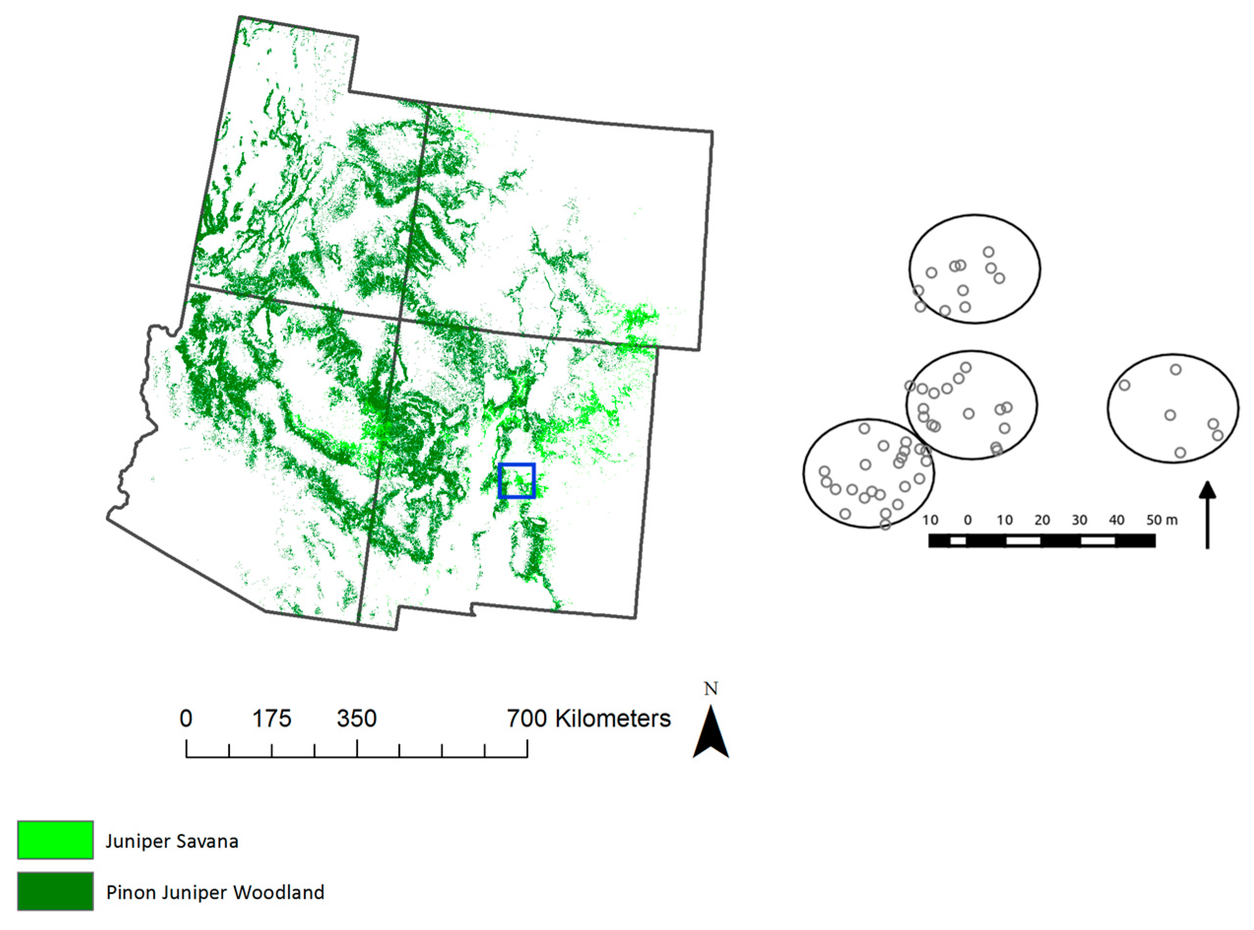
2.1. Site Description

Our study site is located in a juniper savanna woodland, 24 km southeast of Willard, NM (34.425489–105.861545; Figure 1). The 4-ha study region exists within a managed rangeland ecosystem, juniper (J. monosperma) as the only woody species present. The dominant soil type is classified as Penistaja fine sandy loam, and the mean annual temperature and mean annual precipitation are 11.0 °C and 340.6 mm, respectively (PRISM Climate Group, Oregon State University). This site exists as part of a larger gradient of ecological research sites referred to as the New Mexico Elevation Gradient (see [31] for a description of the gradient).

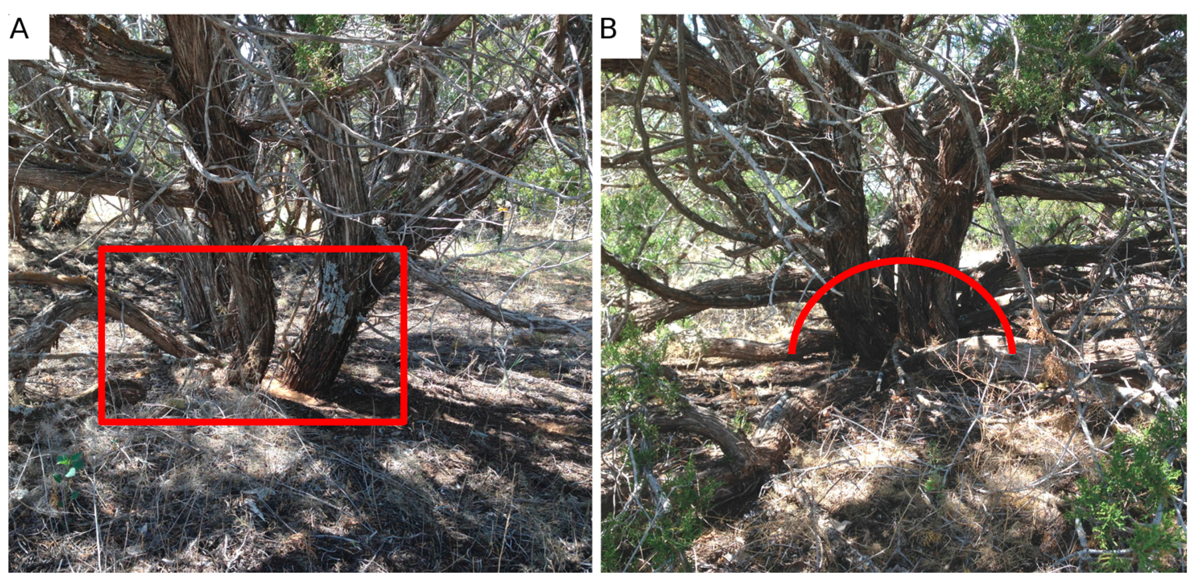
2.2. Field Measurements

The canopy dimensions of all J. monosperma over 1 m in height in four 17.5-m radius circle plots were measured annually at this site from 2007–2014. We mapped the location of 52 individuals in these circle plots (see Figure 1) using a Trimble GPS (following differential correction, RMSE = 40 cm). Canopy height, canopy area and canopy volume, as well as the diameter of the root crown of each tree were measured. Canopy height was measured using a collapsible height stick. Crown area was calculated by measuring the widest diameter and corresponding orthogonal dimension. The entire projected crown volume then was calculated given the height and subsequent projected area of the ellipsoid. The stem diameter of J. monosperma is challenging to measure given the complex growth morphology of individuals. The bole of the tree can either branch above (Figure 2A) or below (Figure 2B) the ground, making measurements of the root collar diameter (RCD, stem basal area at the base of the plant) inconsistent if conducted at the ground level. The diameter at breast height (DBH) is often impractical to estimate on this species given that height results in increasingly complex branching patterns. However, the allometry from [32] specifies that the equivalent stem diameter be recorded at the root collar (Equation (1)), where ESD is equivalent stem diameter computed as the sum of the square of each root collar diameter (RCDi, present for an individual). Therefore, we chose to measure the stem diameter of individuals roughly 30 cm radially up and out from the bole (Figure 2B). In this manner, the woody mass often found at the base of those junipers that branch above ground would not bias the ESD measurements.
E S D = i = 1 n R C D i 2

2.3. Airborne LiDAR Data

On 8 September 2011, high resolution airborne LiDAR was collected across a 6.5-km2 area situated along a 5-km north-south extent that included the 4-ha study area. Using an Optech Gemini with a laser pulse repetition rate of 125 kHz, 50% flight-line overlap, scan angle of ±16° and flying at an average altitude of 400 m above ground, LiDAR data were collected over the juniper savanna site. The LiDAR point cloud data had an average horizontal point spacing of 20 cm and a point density of 10 points·m−2. The mean horizontal relative accuracy was 25 cm RMSE, and vertical accuracy was approximately 10 cm RMSE or better for open surfaces. Figure 3A shows the full analysis extent.

2.4. Canopy Segmentation and Statistics

A digital terrain model (DTM) was extracted using the Terrain Extraction and Segmentation (TEXAS) software developed by the University of Texas’ Applied Research Laboratories [33]. The utilization of an accurate terrain model is critical for estimating the height of vegetation above the ground surface. Once a DTM was generated and the point height above the ground was calculated, the individual points within the LiDAR point cloud were analyzed and labeled into general land cover categories, such as vegetation, terrain or man-made surfaces (Figure 4A) using the TEXAS Point cloud Exploitation Research Toolbox (TEXPERT, [33]).
LiDAR points classified as vegetation were then grouped into segments based on their Euclidean distance to matching adjacent points. The DTM provided a reference point for segmenting vegetation, allowing for all points with some height above the DTM to be grouped as vegetation. This process results in a highly accurate vegetation/bare earth segmentation when working in simple systems, like savannas. The resulting segmentation was visually assessed for accuracy within the study area using high resolution satellite imagery (user’s and producer’s accuracies of >98% for classification of vegetation taller than 1 m). For this project, vegetation points were grouped as a segment if a neighboring vegetation point was within 1 m (e.g., Figure 4B), an empirically-derived threshold that was based on the acquisition point density and vegetation density across the plot. Height statistics computed on the LiDAR points within each segment include the standard metrics (i.e., mean, max, median and standard deviation of height (m)). Other segment statistics included projected canopy area (m2), perimeter (m), canopy volume (m3), canopy density (points·m−3), canopy closure (unitless) and eccentricity (unitless). Canopy volume is defined as the projected canopy area multiplied by the maximum canopy height. Here, we define canopy closure as the ratio of canopy returns to ground returns within the projected area of each segment. If a segment has a well-defined major and minor axis, the eccentricity is computed for each segment. Trees and clumps with a near circular shape should have an eccentricity near zero, whereas more elliptically-shaped trees and clumps will have eccentricities near 0.5. The strength of these metrics is that they are computed on all of the points within the segmented point cloud rather than only the first reflective surface, as in a canopy height model.
A vectorized version of the segmentation (i.e., the perimeter of each clump) was then produced and overlaid with the ground-based tree location data (Figure 4C).The maximum height from each tree crown within the field-measured circle plots was manually retrieved and regressed against the corresponding field heights to assess the uncertainty in the ground-LiDAR height relationship. To further test how spatially representative our field measurement area was, we assessed the LiDAR-derived max canopy heights by running a 7 m × 7 m kernel local maximum filter across the analysis extent and comparing the resulting distribution of heights against the field-collected height data.

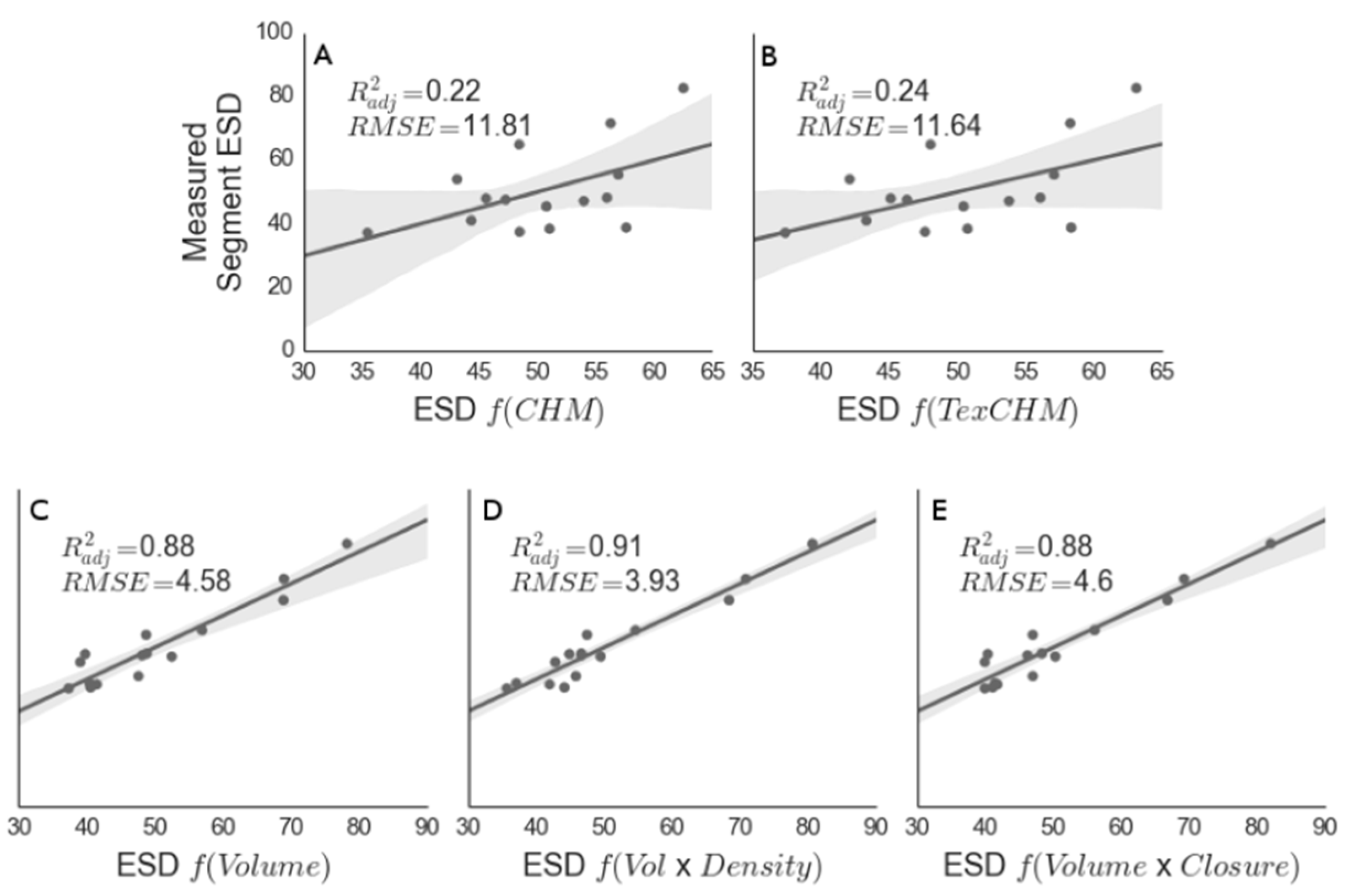
2.5. Validation of Clump Level Allometries

Estimates of stem diameter were scaled to the remote sensing data (i.e., the LiDAR-derived segmentation) using an empirical regression between ESD and single tree crown volume derived from the ground measurements. Given that the LiDAR segmentation approach delineated either individual or small clumps of trees, the ability of the regressions to predict the cumulative stem diameters of our ground validation trees needed to be determined. GPS-collected tree locations were visually inspected to associate segmented canopy objects with corresponding ground validation data. In some cases, LiDAR-derived canopy segments included trees that were not sampled within the four 17.5-m radius circle plots, reducing our effective sample size. In these cases, the entire LiDAR-derived segment was removed from the validation set to avoid biasing the regression. For the remaining trees, the cumulative crown volumes and stem diameters were calculated and regressed against the LiDAR-derived segmented approximations. LiDAR-derived segment volumes were estimated from the projected segment area and the maximum height within each segment. We also included canopy closure and canopy density computed on a per segment basis as additional covariates to the linear regression. Regression goodness of fits were compared using both the adjusted R2 (R2ADJ) and root mean squared error (RMSE).

2.6. Uncertainty Estimation

We chose a simplified Monte Carlo approach to propagate error, adapted from [34]. We used the regression standard error from the segment volume to segment ESD linear fit (RMS), as well as the published standard error of prediction from the allometry for J. monosperma from [32] as our sources of error. For each crown segment, we then computed 1000 realizations of segment ESD with random perturbations in the error term. This was done by randomly drawing from a normal distribution (mean of 0, scale of 1) and multiplying that random number by the RMS for either the appropriate model regression. Each of these randomly-generated uncertainties was then added to the original source of error for the propagation workflow. Each of the 1000 realizations was then used to generate estimates of biomass, using the previously-published allometric uncertainty [32], which we randomly perturbed in the same manner. We then calculated the biomass of each segment from a mean of 1000 model runs, and the associated standard deviation of each segment was carried through to compute the uncertainty in biomass prediction using confidence intervals.

3. Results

3.1. Field Measurements

The mean canopy height, area, volume and ESD were 3.7 m, 26.2 m2, 70.6 m3 and 32.5 cm, respectively (Figure 5), with an estimated stem density within our four-hectare analysis region of 135.1 stems·ha−1. The representativeness of the trees used to parametrize the LiDAR-based regressions of biomass was assessed by comparing field-measured canopy height with the mean local maximum canopy height within the LiDAR analysis extent, and the distribution of heights measured by our field plots was representative of the analysis extent (Figure 6). The mean estimated field biomass using the allometry from Grier et al. [32] was 15.6 megagrams per hectare (Mg·ha−1). The three ground-measured crown properties (height, area and volume) all performed well as predictors of single tree ESD, with adjusted R2ADJ values of 0.60, 0.77 and 0.80, respectively (p < 0.001). We chose to use canopy volume to drive our remote allometry (Figure 7), as it was the best predictor of ESD (R2ADJ = 0.79, RMSE = 1.23 cm2, p < 0.001). The resulting regression equation was:
log ( E S D ) = 0.43 × log ( V o l u m e ) + 1.72

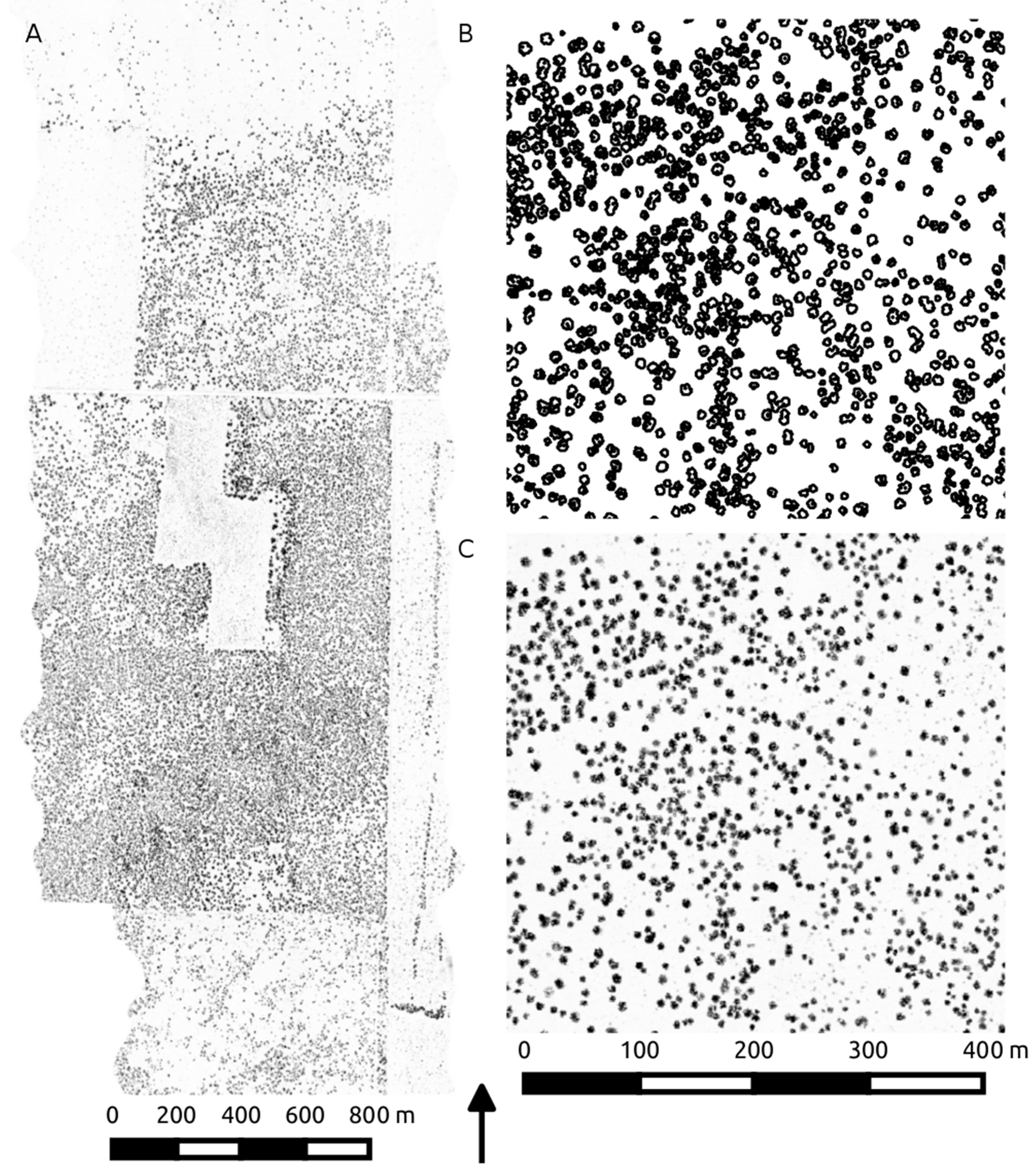
3.2. LiDAR Segmentation

The TEXPERT-derived segmentation identified a total of 3655 objects, each representing one or several crowns within the analysis extent (see Table 1 for summary statistics for the entire region). The TEXPERT segmentation tended to clump multiple individuals into a single segment (under-segmentation), with multiple segments per individual (over-segmentation) occurring in very few cases. In the rare case of over-segmentation within the ground control plots, we clumped the segments that corresponded to ground-measured individuals in order to drive the segment volume to ESD relationship. Large segments had a higher likelihood of containing multiple individuals, but in the case of the 4-ha region used for ground validation, the number of individuals per segment was not significantly explained by segment volume, perimeter or area. Contiguous swaths of vegetation tended to segment together, given that the segmentation was driven by the similarity of canopy height. Within our ground validation region, the arrangement of ground-mapped individuals within segmented clumps corresponded well with the segmentation, where standalone individuals were properly segmented, and overlapping crowns were grouped accordingly (e.g., Figure 4C). The four 17.5-m radius circle plots contained a total of 19 segmented crown objects, composed of 52 individuals.

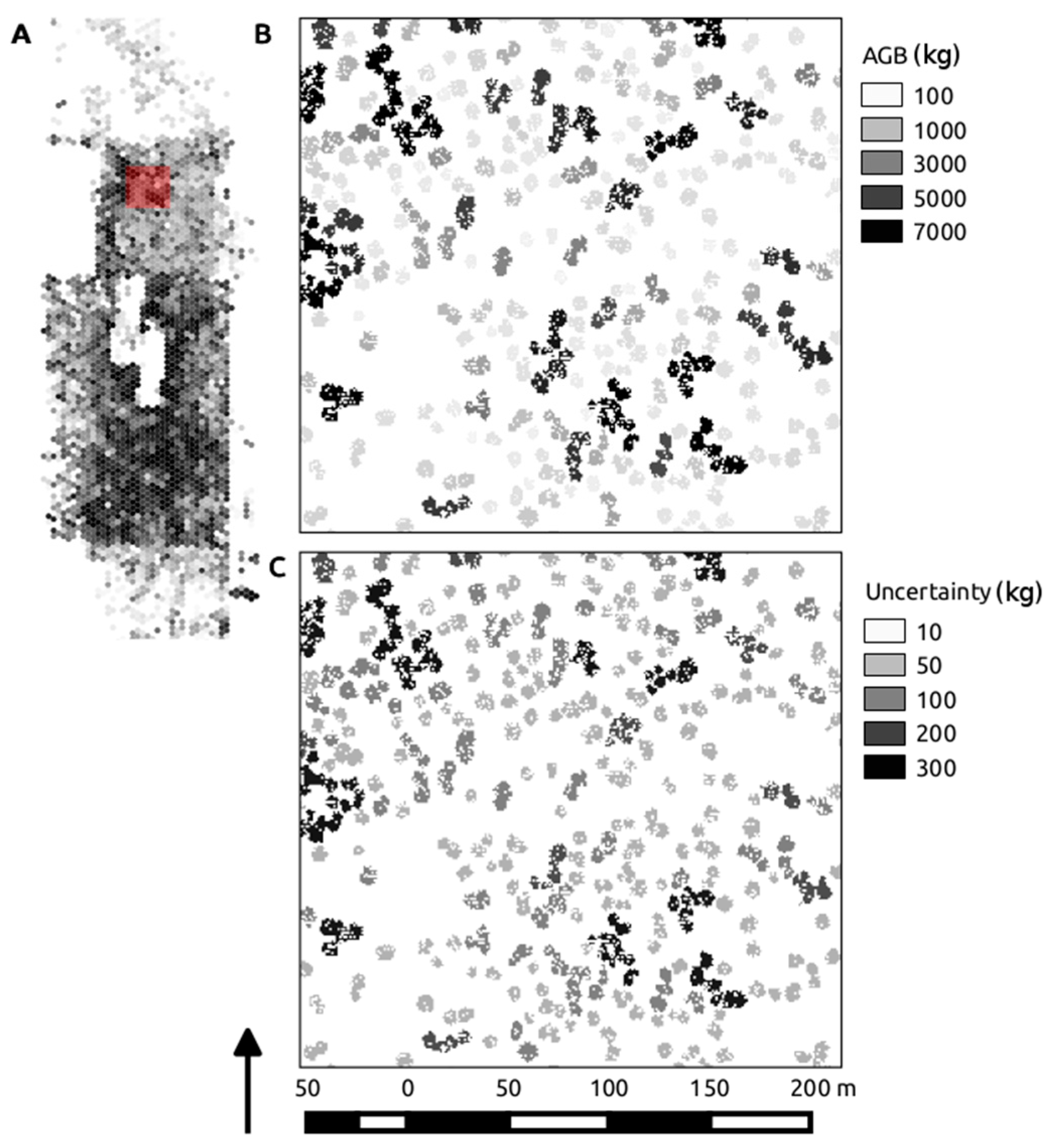
3.3. Segmentation-Derived Biomass and Uncertainty

We clumped the field measurement data according to the corresponding segments in which the field-measured crowns were located, permitting the calculation of a ‘whole clump’, cumulative ESD. We used the cumulative ESD as validation data for five separate linear regressions (Table 2). The first two models were driven by maximum segment height only, with HCHM and HTEX corresponding to maximum segment height derived via the surface height raster (2D) and the full point cloud (3D), respectively. The final three models were driven by TEXPERT-derived 3D point cloud statistics (Vol = volume only, VolD = volume and point density, VolC = volume and segment closure). Neither HCHM nor HTEX predictions of ESD showed relationships with ground-measured clumped ESD, which were commensurate with the ground-driven individual regressions (Figure 7A compared to Figure 8A,B), suggesting that the linearity imposed by log transforming the ground data is lost when scaling to multiple individuals. The 3D point cloud-derived height estimates from HTEX did show an improved fit relative to the raster-derived estimates from HCHM (R2ADJ = 0.22 vs. 0.24, p < 0.05), yet neither model showed correlations that were significantly improved relative to the volume-based models.
All of the models driven by segment volume performed well (Figure 8). Volume alone was a strong predictor of ESD in juniper clumps (Vol R2ADJ = 0.89, p < 0.001), yet when segment point density was included as a covariate in the regression, the correlation between predicted and measured ESD increased and the RMSE decreased, in spite of the increasing model complexity (VolD R2ADJ = 0.91, p < 0.001; Figure 8C). Canopy closure did not show a significant improvement over the volume-only model (Table 2). Using the VolD model structure, the resulting 95th percentile confidence interval for the estimated total biomass over the field measurement extent was calculated as 14.7 ± 0.13 Mg·ha−1 compared to the field-measured mean of 15.6 Mg·ha−1, where uncertainty is expressed as the mean standard deviation from each segment’s AGB estimate output from the Monte Carlo approach described in Section 2.6. On a per-segment basis, the AGB estimates and corresponding segment standard deviations from the VolD model were well distributed and reasonable given our knowledge of the site (Figure 9).
Given that the propagation of error throughout the analysis incorporated both the remote prediction of ESD, as well as the allometric uncertainty in AGB prediction, the relationship between segment AGB standard deviation followed an exponential relationship with mean segment AGB. Across the analysis extent, the distribution of biomass and consequently uncertainty is strongly a function of segment size, influenced primarily by continuity in the structural features of the canopy, such as stem density and variability in canopy height. The resulting mapped biomass illustrates both the results of AGB mean and standard deviation resampled to roughly 1-ha cells driven by the model VolD (Figure 10A,B), as well as the difference between the Vol and VolD outputs (Figure 10C), which corresponds to roughly 2.6 Mg·ha−1 across the analysis extent.

4. Discussion

We showed that the scaling of the measured ESD between individuals as a function of LiDAR-derived segment volume produced estimations of AGB that matched single tree allometry-derived predictions. Using canopy object density as a covariate to constrain the relationship between ESD and canopy volume not only improved the statistical power of the model, but also clarified the conceptual model relationship as:
ESD = Segment Volume × Segment Density
Therefore, the inclusion of segment point density, derived from the LiDAR point cloud, increased the quality of the relationship between field-measured and clump-estimated ESD (Figure 8), which improved with the additional parameter in spite of increasing model complexity (R2ADJ = 0.91).
Our field measurements of J. monosperma were highly representative of the entire analysis extent, given the similarities in single crown maximum height and the distributions of LiDAR- and field-derived tree height. Further, the similarity between the LiDAR-derived heights and the field-measured heights for the 52 trees measured in this study showed good agreement (R2 of 0.79, p < 0.001), consistent with the good agreement seen in previous studies (e.g., [35,36]). Potential sources of error between field-measured crown parameters and those derived from LiDAR are potentially due to the horizontal resolution of the LiDAR data (1 m), effectively smoothing maximum heights and canopy edges, and to errors in the ground data collection. Higher resolution data may constrain the absolute error associated with measuring canopy heights, but agreement with field measurements may not improve unless the sophistication of the field height estimates increases (e.g., with the use of a laser hypsometer rather than a collapsible height stick). Our sample size for the regressions used to assess the goodness of fit at the segmentation level was greatly reduced relative to our ground validation sample size (n = 52 for field regressions, n = 15 for segmentation-based regressions) given that in most cases, single canopy objects derived from LiDAR were actually comprised of multiple individuals. Further, our circle plot-based validation approach poorly accommodated segmented canopy objects, which spanned the circle plot perimeter, reducing the number of segments we were able to include in the predictive models. This small sample size may reduce our ability to scale these results to areas further reaching than our immediate analysis area. However, we believe the method we employed is scalable and that the general results of increasing explanatory power by leveraging the full point cloud data would not fall apart had we increased our sampling number.
The relationship we developed between crown volume and equivalent stem diameter (ESD; Equation (2)), corresponds well with our field-measured trees, with nearly 90% of the variance in ESD explained by canopy volume. This seems intuitive given the morphology of the trees (Figure 2), which grow more like large shrubs in this ecosystem. The complication in scaling this relationship using the LiDAR-derived segments is that the segmentation only produces crown-shaped objects when the vegetation is isolated on the landscape. In many instances, however, juniper grows in clumps of several trees. By using structural metrics derived from the LiDAR 3D point cloud, such as canopy volume, canopy density and canopy closure, we showed that the cumulative ESD and, subsequently, AGB agreed well with field-measured estimates for a vegetation clump. This result demonstrates that a single tree segmentation may not be required to estimate biomass in juniper-dominated ecosystems. Because the segmentation was actually conducted on the full 3D point cloud, each canopy object carried with it a host of ancillary data (Table 1) that reduced the need for single tree segmentation. Further, the power law relationship between stem diameter and crown volume necessitates log transforming ground-based measurements to apply linear fits (e.g., Figure 7). When scaling ESD to the level of vegetation clumps, the relationship between whole clump volume and whole clump ESD is inherently linear, further increasing the simplicity and ease of use of this relationship (e.g., Figure 8). Unfortunately, we did not test this for arbitrarily large segments, and presumably, the scaling of single crown allometrics across increasingly large canopy objects will increase the uncertainty of the estimation. However, the TEXPERT segmentation process performed consistently in sparse, clumped systems, constraining the variability in segment size across the scene.
The use of active sensors, such as airborne LiDAR, historically has improved the remote estimate of above ground biomass by relating destructive harvesting with plot scale measurements of height or fractional cover of vegetation (e.g., [37]). This approach also often hinges on individual tree crown delineation (e.g., [8]), and the resulting segment statistics are used as coefficients in a regression against harvested or allometrically-estimated biomass. In highly clumped vegetation, such as piñon-juniper (PJ) woodlands or juniper savannas, the accuracy of single tree segmentation is difficult to quantify, and consequently, scaling relationships designed for single crowns could be introducing systematic errors to the biomass estimation if, for instance, multiple woody boles are lumped into a single crown volume or tree segment height estimate. Our results suggest that the use of a segmentation conducted on the full 3D point cloud can produce accurate estimates of AGB even when multiple trees are clumped in a single segment.
This work contributes to the challenging task of remotely estimating AGB in juniper-dominated systems. Future work in juniper and juniper co-dominated woodlands (e.g., PJ woodlands) could benefit from this approach, specifically by conducting the single or clumped crown segmentation on the full 3D point cloud and preserving the within-clump LiDAR-derived statistics. However, mixed species allometries are inherently less accurate than their single species counterparts, as remotely leveraging single species allometries in a structurally-complex ecosystem like a PJ woodland would require the ability to not only delineate crowns consistently, but also to identify the difference between juniper and piñon or to determine an accurate mixed species allometry. This method holds potential for application in other open systems, such as oak savannas, less arid woodlands and plantations. In such systems, the over-story structure of vegetation is normally composed of one or two pant functional types, and segmenting the vegetation into appropriate groups would be operationally simple. In systems with more vertical structure, such as conifer or deciduous forests, the segmentation process may begin to introduce too much error into the workflow to make the approach worthwhile.

5. Conclusions

Rapid and accurate remotely-sensed estimations of ecosystem AGB are now more than ever a critical component to climate change mitigation strategies in the southwestern U.S. Given the spatial extent of Juniperus spp. across the region and the complex growth morphology exhibited by the genus, improving our ability to estimate the AGB of juniper-dominated systems will provide valuable information about a range of ecosystems that will potentially undergo significant changes in structure at the ecosystem scale. Our case study in a juniper savanna demonstrated the ability of LiDAR data to drive existing stem diameter-based allometries remotely, using an object-based approach. Given that delineating individual crowns in systems characterized by highly clumped vegetation is a challenging and error-prone process, we scaled ground-derived allometries based on crown volume to segmented groups of individuals. By driving the segmentation process on the full 3D point cloud data from LiDAR, we were able to refine the regression between segment volume and stem diameter using the density of points per segment. This work illustrates the capability of segmentation approaches delineating groups of individuals rather than single crowns to scale the existing AGB allometric relationship at the regional scale. While we believe this approach can both simplify the typical demand for crown level segmentation, and constrain AGB prediction uncertainty by leveraging 3D statistics per canopy segment, more work will be required to apply the technique in mixed species, highly clumped ecosystems, such as PJ woodlands.

Acknowledgments

This work was funded by NASA Grant NX11G91G. We would like to thank the 7-up 7-down ranch for generously allowing us the use of their land. We would also like to thank Johnathan Furst and Stephanie Schmiege at the University of New Mexico for their hard work and contributions in data collection and processing.

Author Contributions

Dan Krofcheck and Marcy Litvak designed the analyses. Christopher Lippitt contributed to the experimental design and statistical analysis. Amy Neuenschwander processed the raw LiDAR data and provided point cloud statistics. Dan Krofcheck wrote the paper.

Conflicts of Interest

The authors declare no conflict of interest.

References

  1. Savage, V.M.; Bentley, L.P.; Enquist, B.J.; Sperry, J.S.; Smith, D.D.; Reich, P.B.; von Allmen, E.I. Hydraulic trade-offs and space filling enable better predictions of vascular structure and function in plants. PNAS 2010, 107, 22722–22727. [Google Scholar] [CrossRef] [PubMed]
  2. West, G.B.; Enquist, B.J.; Brown, J.H. A general quantitative theory of forest structure and dynamics. PNAS 2009, 106, 7040–7045. [Google Scholar] [CrossRef] [PubMed]
  3. Swetnam, T.L.; Falk, D.A.; Lynch, A.M.; Yool, S.R. Estimating individual tree mid- and understory rank-size distributions from airborne laser scanning in semi-arid forests. Forest Ecol. Manag. 2014, 330, 271–282. [Google Scholar] [CrossRef]
  4. Poulter, B.; Frank, D.; Ciais, P.; Myneni, R.B.; Andela, N.; Bi, J.; Broquet, G.; Canadell, J.G.; Chevallier, F.; Liu, Y.Y.; et al. Contribution of semi-arid ecosystems to interannual variability of the global carbon cycle. Nature 2014, 509, 600–603. [Google Scholar] [CrossRef] [PubMed]
  5. Gibbs, H.K.; Brown, S.; Niles, J.O.; Foley, J.A. Monitoring and estimating tropical forest carbon stocks: Making REDD a reality. Environ. Res. Lett. 2007, 2, 045023. [Google Scholar] [CrossRef]
  6. Jenkins, J.; Chojnacky, D.; Heath, L.; Birdsey, R. Comprehensive Database of Diameter-Based Biomass Regressions for North American Tree Species. Available online: http://svinet2.fs.fed.us/ne/durham/4104/papers/ne_gtr319_jenkins_and_others.pdf (assessed on 18 May 2016).
  7. Chojnacky, D.C.; Heath, L.S.; Jenkins, J.C. Updated generalized biomass equations for North American tree species. Forestry 2013, 87, 129–151. [Google Scholar] [CrossRef]
  8. Colgan, M.S.; Asner, G.P.; Swemmer, T. Harvesting tree biomass at the stand level to assess the accuracy of field and airborne biomass estimation in Savannas. Ecol. Appl. 2013, 23, 1170–1184. [Google Scholar] [CrossRef] [PubMed]
  9. Goetz, S.J.; Baccini, A.; Laporte, N.; Johns, T.; Walker, W.; Kellendorfer, J.; Houghton, R.; Sun, M. Mapping and monitoring carbon stocks with satellite observations: A comparison of methods. Carbon Balance Manag. 2009, 4, 2. [Google Scholar] [CrossRef] [PubMed]
  10. Hansen, M.; Potapov, P.; Moore, R.; Hancher, M.; Turubanova, S.; Tyukavina, A.; Thau, D.; Stehman, S.; Goetz, S.; Loveland, T.; et al. High-resolution global maps of 21st century forest cover change. Science 2013, 342, 6160. [Google Scholar] [CrossRef] [PubMed]
  11. Krofcheck, D.J.; Eitel, J.U.H.; Vierling, L.A.; Schulthess, U.; Hilton, T.M.; Dettweiler-Robinson, E.; Litvak, M.E. Detecting mortality induced structural and functional changes in a piñon-juniper woodland using Landsat and RapidEye time series. Remote Sens. Environ. 2014, 151, 102–113. [Google Scholar] [CrossRef]
  12. Mascaro, J.; Detto, M.; Asner, G.P.; Muller-Landau, H.C. Evaluating uncertainty in mapping forest carbon with airborne LiDAR. Remote Sens. Environ. 2011. [Google Scholar] [CrossRef]
  13. Eckert, S. Improved forest biomass and carbon estimations using texture measures from WorldView-2 satellite data. Remote Sens. 2011, 4, 810–829. [Google Scholar] [CrossRef]
  14. Asner, G.P.; Archer, S.; Hughes, R.F.; Ansley, R.J.; Wessman, C.A. Net changes in regional woody vegetation cover and carbon storage in Texas Drylands, 1937–1999. Glob. Chang. Biol. 2003, 9, 316–335. [Google Scholar] [CrossRef]
  15. Browning, D.M.; Archer, S.R.; Asner, G.P.; McClaran, M.P.; Wessman, C.A. Woody plants in grasslands: post-encroachment stand dynamics. Ecol. Appl. 2008, 18, 928–944. [Google Scholar] [CrossRef] [PubMed]
  16. Mirik, M.; Chaudhuri, S.; Surber, B.; Ale, S.; Ansley, R. Evaluating Biomass of Juniper Trees (Juniperus pinchotii) from Imagery-Derived Canopy Area Using the Support Vector Machine Classifier. Adv. Remote Sens. 2013, 2, 181–192. [Google Scholar] [CrossRef]
  17. Means, J.E.; Acker, S.A.; Fitt, B.J.; Renslow, M.; Emerson, L.; Hendrix, C.J. Predicting forest stand characteristics with airborne scanning LiDAR. Photogramm. Eng. Remote Sens. 2000, 66, 1367–1371. [Google Scholar]
  18. Næsset, E.; Gobakken, T. Estimation of above- and below-ground biomass across regions of the boreal forest zone using airborne laser. Remote Sens. Environ. 2008, 112, 3079–3090. [Google Scholar] [CrossRef]
  19. Packalen, P.; Vauhkonen, J.; Kallio, E.; Peuhkurinen, J.; Pitkanenm, J.; Pippuri, I.; Strunk, J.; Maltamo, M. Predicting the spatial pattern of trees by airborne laser scanning. Int. J. Remote Sens. 2013, 34, 5145–5165. [Google Scholar] [CrossRef]
  20. Swetnam, T.L.; Falk, D.A. Application of metabolic scaling theory to reduce error in local maxima tree segmentation from aerial LiDAR. Forest Ecol. Manag. 2014, 323, 158–167. [Google Scholar] [CrossRef]
  21. Sankey, T.T.; Glenn, N.; Ehinger, S.; Boehm, A.; Hardegree, S. Characterizing western juniper expansion via a fusion of Landsat 5 Thematic Mapper and LiDAR data. Rangel. Ecol. Manag. 2010, 63, 514–523. [Google Scholar] [CrossRef]
  22. Sankey, T.; and Glenn, N. Landsat-5 TM and LiDAR fusion for sub-pixel juniper tree cover estimates in a western rangeland. Photogr. Eng. Rempte Sens. 2011, 77, 1241–1248. [Google Scholar] [CrossRef]
  23. Wessels, K.J.; Erasmus, B.F.N.; Colgan, M.; Asner, G.P.; Mathieu, R.; Twine, W.; Van Aardt, J.A.N.; Smit, I. Impacts of communal fuelwood extraction on LiDAR-estimated biomass patterns of savanna woodlands. Int. Geosci. Remote Sens. 2012, 1676, 1679. [Google Scholar]
  24. Sankey, T.; Shrestha, R.; Sankey, J.B.; Hardegree, S.; Strand, E. LiDAR-derived estimate and uncertainty of carbon sink in successional phases of woody encroachment. J. Geophys. Res. Biogeosci. 2013, 118. [Google Scholar] [CrossRef]
  25. Swetnam, T.W.; Allen, C.D.; Betancourt, J.L. Applied historical ecology: Using the past to manage for the future. Ecol. Appl. 1999, 9, 1189–1206. [Google Scholar] [CrossRef]
  26. Miller, R.F.; Tausch, R.J. The role of fire in juniper and pinyon woodlands: A descriptive analysis. In Proceedings of the Invasive Species Workshop: Fire Conference 2000: The First National Congress on Fire Ecology, Prevention, and Management, San Diego, CA, USA, 27 November–1 December 2000.
  27. Allen, C.D.; Macalady, A.K.; Chenchouni, H.; Bachelet, D.; McDowell, N.; Vennetier, M.; Kitzberger, T.; Rigling, A.; Breshears, D.D.; Gonzalez, P.; et al. A global overview of drought and heat-induced tree mortality reveals emerging climate change risks for forests. Forest Ecol. Manag. 2010, 259, 660–684. [Google Scholar] [CrossRef]
  28. Breshears, D.; Rich, P. Overstory-imposed heterogeneity in solar radiation and soil moisture in a semiarid woodland. Ecol. Appl. 1997, 4, 1201–1215. [Google Scholar] [CrossRef]
  29. Clifford, M.; Rocca, M.; Delph, R. Drought induced tree mortality and ensuing Bark beetle outbreaks in Southwestern pinyon-juniper woodlands. In USDA Forest Service Proceedings; US Forest Service: Washington, DC, USA, 2008. [Google Scholar]
  30. Clifford, M.; Royer, P.; Cobb, N. Precipitation thresholds and drought-induced tree die-off: Insights from patterns of Pinus edulis mortality along an environmental stress gradient. New Phytol. 2013, 200, 413–421. [Google Scholar] [CrossRef] [PubMed]
  31. Anderson-Teixeira, K.J.; Delong, J.P.; Fox, A.M.; Brese, D.A.; Litvak, M.E. Differential responses of production and respiration to temperature and moisture drive the carbon balance across a climatic gradient in New Mexico. Glob. Chang. Biol. 2011, 17, 410–424. [Google Scholar] [CrossRef]
  32. Grier, C.C.; Elliott, K.J.; Mccullough, D.G. Biomass distribution and productivity of Pinus edulis-Juniperus monosperma woodlands of north-central Arizona. Forest Ecol. Manag. 1992, 50, 331–350. [Google Scholar] [CrossRef]
  33. Stevenson, T.H.; Magruder, L.A.; Neuenschwander, A.L.; Bradford, B. Automated bare earth extraction technique for complex topography in light detection and ranging surveys. J. Appl. Remote Sens. 2013, 7, 073560. [Google Scholar] [CrossRef]
  34. Gonzalez, P.; Asner, G.P.; Battles, J.J.; Lefsky, M.A.; Waring, K.M.; Palace, M. Forest carbon densities and uncertainties from LiDAR, Quickbird, and field measurements in California. Remote Sens. Environ. 2010, 114, 1561–1575. [Google Scholar] [CrossRef]
  35. Weltz, M.A.; Ritchie, C.; Fox, H.D. Comparison of laser and field measurements of vegetation height and canopy cover watershed precision vegetation properties height and canopy. Water Resour. Res. 1994, 30, 1311–1319. [Google Scholar] [CrossRef]
  36. Colgan, M.S.; Swemmer, T.; Asner, G.P. Structural relationships between form factor, wood density, and biomass in African savanna woodlands. Trees 2013, 28, 91–102. [Google Scholar] [CrossRef]
  37. Fernandez, D.P.; Neff, J.C.; Huang, C.-Y.; Asner, G.P.; Barger, N.N. Twentieth century carbon stock changes related to Piñon-Juniper expansion into a black sagebrush community. Carbon Balance Manag. 2013, 8, 8. [Google Scholar] [CrossRef] [PubMed]
Figure 1. Extent of piñon juniper woodlands (PJ, dark green) and juniper savanna (JSAV, light green) ecosystems across the four corner states. (Right) Location and layout of the field site, with tree crown locations bounded by the four 17.5-m radius circle plots.
Remotesensing 08 00453 g001
Figure 2. Typical branching patterns of Juniperus monosperma across the study area. Some individuals branch below the ground (A), while others branch above (B). Due to the woody mass that sometimes forms at the base of these trees, we measured equivalent stem diameters (ESD; Equation (1)) as illustrated in (B), using an ~30-cm radius from the woody mass to each stem diameter measurement.
Remotesensing 08 00453 g002
Figure 3. LiDAR canopy height acquisition extent (A) displayed as a canopy height raster. The corresponding TEXPERT segmentation (B) represents the delineated isolated and clumped crowns, used to generate canopy statistics on the raw height and volume data (C).
Remotesensing 08 00453 g003
Figure 4. (A) The automatic delineation of ground and vegetation from the TEXAS model, resulting in (B) clumped crown segmentation, which was then (C) vectorized and overlaid on ground-measured stem maps within our study area for segment statistic generation.
Remotesensing 08 00453 g004
Figure 5. Distributions of juniper canopy parameters retrieved via ground measurement.
Remotesensing 08 00453 g005
Figure 6. Distributions of juniper canopy parameters retrieved via analysis of the LiDAR data.
Remotesensing 08 00453 g006
Figure 7. Ground-derived relationships between canopy parameters and equivalent stem diameter (ESD; see Equation (1)). Both axes have been log transformed to establish linear fits.
Remotesensing 08 00453 g007
Figure 8. Modeled equivalent stem diameter (ESD; Equation (1)) versus measured stem diameter. Here, the modeled stem diameter was generated using max height from the raster canopy height model (CHM) (A); max height from the TEXPERT height model (B); segment volume from TEXPERT (C); volume and density (D); and volume and closure (E). RMSE is expressed in units of cm.
Remotesensing 08 00453 g008
Figure 9. Overview map of the study extent, displaying Mg AGB binned into roughly 0.08-ha hexels, highlighted by the red extent marker (A); the individual segment calculations of kg AGB driven by the best performing model (VolD) are shown in (B); with the corresponding segment standard deviation in kg shown in (C).
Remotesensing 08 00453 g009
Figure 10. Mapped mean biomass (Mg AGB) binned into roughly 0.08-ha hexels across the analysis extent derived from the best predictors of equivalent stem diameter, volume and density (A) and the corresponding mean standard deviation for the mean AGB in each hex (B); (C) highlights the difference between biomass predictions using ESD as a function of volume only, vs. ESD derived from volume and density, calculated as VolVolD, where the resulting difference is expressed in terms of Mg AGB.
Remotesensing 08 00453 g010
Table 1. Summary of the clumped segmentation statistics generated from the full 3D point cloud for all of the canopy objects within the analysis extent. Abbreviations: Standard Deviation (Std), Average (Avg).
Segment StatisticMinMaxMeanStd
Max Elevation (m)1.558.314.140.76
Min Elevation (m)03.440.30.09
Avg Elevation (m)0.575.672.120.37
Med Elevation (m)0.227.362.281.06
Std Elevation (m)0.282.381.020.23
RMS Elevation (m)0.645.772.360.4
Perimeter (m)10.97290.4542.0824.43
Projected Area (m2)12.672158.1394.35117.73
Volume (m3)41.335302.16399.52611.66
Density (unitless)0.080.990.440.21
Closure (unitless)0.1710.750.15
Table 2. Predictive model structures tested in the study. Models driven by height or volume alone contain only a slope (α) and intercept (b) as parameters, whereas models with two inputs (VolD and VolC) contain an additional primary and interaction term (β and γ). ESD, equivalent stem diameter.
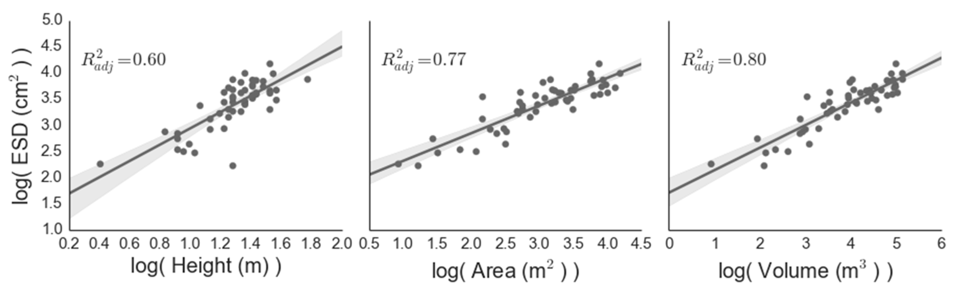
ESD = b + α (x1) + β (x2) + γ (x1 × x2)
Modelx1x2bαβγR2ADJp
HCHMCHM Height-−3.0514.04--0.220.046
HTEXTEX Height-−10.0715.73--0.240.038
VolVolume-31.430.08--0.89<0.0001
VolDVolumeDensity6.410.1642.17−0.150.91<0.0001
VolCVolumeClosure11.2111.2126.65−0.180.89<0.0001

