Improved Quality of MODIS Sea Surface Temperature Retrieval and Data Coverage Using Physical Deterministic Methods

Abstract

Sea surface temperature (SST) retrievals from satellite imager measurements are often performed using only two or three channels, and employ a regression methodology. As there are 16 thermal infrared (IR) channels available for MODIS, we demonstrate a new SST retrieval methodology using more channels and a physically deterministic method, the modified total least squares (MTLS), to improve the quality of SST. Since cloud detection is always a part of any parameter estimation from IR satellite measurements, we hereby extend our recently-published novel cloud detection technique, which is based on both functional spectral differences and radiative transfer modeling for GOES-13. We demonstrate that the cloud detection coefficients derived for GOES-13 are working well for MODIS, while further improvements are made possible by the extra channels replacing some of the previous tests. The results are compared with available operational MODIS SST through the Group for High Resolution SST website–the data themselves are originally processed by the NASA Goddard Ocean Biology Processing Group. It is observed the data coverage can be more than doubled compared to the currently-available operational product, and at the same time the quality can be improved significantly. Two other SST retrieval methods, offline-calculated coefficients using the same form of the operational regression equation, and radiative transfer based optimal estimation, are included for comparison purposes.

1. Introduction

Most operational sea surface temperature (SST) retrievals from satellite measurements are still performed using regression-based methods and, over the years, there has been only limited progress. Such approaches were justifiable in the interest of time and computational resources when they were formulated (e.g., [1,2]). However, this approach is understandably inadequate to attempt to characterize global geophysical conditions (atmospheric and oceanic states) for SST retrievals using only a few regression coefficients. The Group for High Resolution SST (GHRSST), which is an international scientific body, has to date provided MODIS SST using only two and/or three channels by employing a direct regression method. Some of the weaknesses that exist with the current MODIS SST methodology have been documented in the literature [3]. The issue of seasonal bias patterns in NLSST-type retrievals is sufficiently problematic for MODIS SST algorithm teams to have attempted to ameliorate the issue with the development of so-called “latband” NLSST coefficients [4]. While it may be possible to reduce the effects by employing such approaches, the underlying cause remains the inherent limitation of the current algorithm methodology. In addition, the highly-desirable task of assigning error associated to individual retrievals is difficult for regression-based SST retrievals. These above-mentioned reasons, together with the availability of improved computational facilities and more channels in advanced instruments, render the development of forward model-based SST retrievals both feasible and desirable.

Forward model-based SST retrievals (e.g., [5]) are aimed at deriving target parameters (e.g., SST and total column water vapor), using an inversion method from satellite measurements. Most such operational forward model-based methods (not only SST) are stochastic approaches, which are based on Bayesian probability theory, or the related one-dimensional variational principle. Such stochastic techniques differ from each other both in the procedure for solving a set of spectrally-independent radiative transfer (RT) equations (e.g., matrix inversion, numerical iteration) and in the choice of ancillary data. These ancillary data are used to constrain the solution (e.g., atmospheric covariance statistics and a priori estimate of the retrieved parameters) and enforce the results. However, such inversion techniques, scientifically, may pose more questions than they provide solutions. To compensate for inconsistent outcomes, it is common practice to include bias corrections based on “model minus observation” [5,6,7], which risks affecting functional physics and increasing the Jacobian error (e.g., [8]) as well as information loss from the deterministic point of view [9], instead of giving further thought to the inverse method. The ‘model minus observation’ is used to adjust the input total column water vapor (TCWV), which is one variable in the retrieval model. The same ‘model minus observation’ is used to correct forward model biases and atmospheric corrections, while later the same residual is used for retrieval [5,6]. There is no scientific literature available yet where one measurement can produce more than one piece of information from the deterministic point of view. This implies that such approaches may undermine the true potential of expensive satellite missions by introducing potentially ambiguous bias removals from the measurement before inversion. When these results do not meet their aspiration, then the validation data are highly screened [6] for sake of the reference error (e.g., the ensemble drifter error is not close to zero mean) to get the desired results. For example, the Centre de Météorologie Spatiale maintains a rolling blacklist of drifters returning suspicious data, and all observations of drifters blacklisted are excluded here during their blacklisted period. Where drifter observations are greater than 5 K different from a climatological mean SST for the time of year and location, or are greater than 3 K different from the operational sea surface temperature and sea ice analysis SST, those particular observations are also excluded [7]. Such practices risk discarding potentially important oceanographic observations (e.g., strong upwelling events, etc.). Therefore, there is an urgent need for implementing a deterministic inverse algorithm for satellite retrievals. We will show in this paper that good retrievals can be achieved using a deterministic method when the truth is far from the initial guess.

2. Data and Method

Two physical and two regression algorithms are considered for this comparison study. The physical retrieval methods are: (a) Modified Total Least Squares (MTLS), which is a deterministic method; and (b) Optimal Estimation method (OEM), which is based on a stochastic paradigm. Near-real-time two-operational MODIS-AQUA SSTs (OPR and OPR4) for nighttime are provided through GHRSST, which is a traditional regression-based product considered for comparison purposes. We also compare the results using our own coefficients calculated offline for the same form of their regression equation for short-wave (SST4) to verify the performance of our forward model-based cloud algorithm (CEM). Speaking strictly scientifically, the study of day-night together is not a significant issue as the radiative transfer physics for both day and night is mature. However, we have restricted this study to night-only retrievals to avert traditional concerns.

2.1. MTLS

The details, descriptions and derivation of MTLS are available in our paper [9]. The key points are as follows:

$${\mathit{x}}_{mtls}={\mathit{x}}_{ig}+{\left({\mathit{K}}^T\mathit{K}+\frac{2\text{log}\left(\mathsf{\kappa }\right)}{{\gamma }_{snr}^2}{\mathsf{\sigma }}_{end}^2\mathit{I}\right)}^{-1}{\mathit{K}}^T\Delta {\mathit{y}}_{\mathsf{\delta }}$$

(1)

And the analytical error calculation for the retrieval is:

$$\Vert e\Vert =\Vert \left({\mathit{M}}_{rm}-\mathit{I}\right)({\mathit{x}}_{true}-{\mathit{x}}_{ig})\Vert +\Vert {\left({\mathit{K}}^T\mathit{K}+\frac{2\text{log}\left(\mathsf{\kappa }\right)}{{\gamma }_{snr}}{\mathsf{\sigma }}_{end}^2 \mathit{I}\right)}^{-1}{\mathit{K}}^T\Vert \langle \Vert (\Delta {\mathit{y}}_{\mathsf{\delta }}-\mathit{K}({\mathit{x}}_{true}-{\mathit{x}}_{ig}))\Vert \rangle$$

(2)

where $\Vert .\Vert$ is the vector or matrix norm, $\mathit{I}$ is the identity matrix, ${\mathit{M}}_{\mathit{r}\mathit{m}}$, is equal to ${\left({\mathit{K}}^T\mathit{K}+\frac{2\text{log}\left(\mathsf{\kappa }\right)}{{\gamma }_{snr}^2}{\mathsf{\sigma }}_{end}^2\mathit{I}\right)}^{-1}{\mathit{K}}^T\mathit{K}$, is the model resolution matrix, and ${\gamma }_{snr}$ is an additional constraint, which is defined in our paper [9]. ${\mathit{x}}_{true}$ is the assumed true parameter, $\mathit{K}$ is the Jacobian, ${\mathsf{\sigma }}_{end}$ is the lowest singular value of $\left[\mathit{K}\Delta {\mathit{y}}_{\mathsf{\delta }}\right]$, $\mathsf{\kappa }$ is the condition number of the Jacobian, $\Delta {\mathit{y}}_{\mathsf{\delta }}$ is the brightness temperature residual (i.e., observation–model) and $\mathit{x}=\left[\begin{array}{c}s\\ w\end{array}\right]$ is used, where, as before, s is the SST and w is the total column water vapor. x_ig is the initial guess of s and w. The expected information content for individual pixel level retrieval can be quantified in terms of degree of freedom in retrieval (DFR) as the trace of ${\mathit{M}}_{\mathit{r}\mathit{m}}$.

The quality indexing (QI) of retrievals is calculated using the value of total analytical error (Equation (2)) in MTLS. Note that the analytical error is the combined error in SST and water vapor. Furthermore, since ${\mathit{x}}_{true}$ is not generally available, it is substituted with ${\mathit{x}}_{mtls}$, and is, therefore, an approximation. For these reasons, mapping between analytic error and validation results (e.g., satellite-in situ buoy data) may not be exact, although these are expected to be correlated. The binning is based on the fixed value of the analytical error (0 < $\Vert e\Vert$ < 1) into 10 bins evenly spaced in a linear scale. If a bin does not get at least 10% of cloud-free data, then it is combined with the subsequent bin. For each bin, the percentage of total matches is based on the cumulative analytical errors. Furthermore, if the total column water vapor is drastically different from the initial guess (IG), it is impossible to find a solution using only a single iteration due to nonlinearity. The last bin is likely to contain a substantial population of “bad” retrievals, i.e., caused by cloud-leakage or other errors in the ancillary information including WV profile shape error. This is implemented using appropriate threshold conditions based on physical understanding of the problem and the increments of s and w output from the MTLS retrieval. The detection of night-time fractional cloud or low level cloud is very difficult, where low brightness temperature (BT) for all measurements will be observed and the MTLS solution will produce a relatively large negative value of s, as well as high w, to compensate for the negative value of the residual. Pixels, where the calculated value of the analytical error is ≥ 1, are also placed in the last bin as bad retrievals. This offers the prospect that such conditions can be detected at solution time, by determining a suitable threshold. Thus, another advantage of the MTLS solution is to facilitate improvement of the cloud and error masking. It should be noted that the total error calculation is unable to account for certain aspects of the statistics obtained with respect to in situ matches, such as surface effects, buoy error, and representativity (point-to-area) error.

2.2. OEM

The OEM solution is briefly stated as:

$${\mathit{x}}_{oe}={\mathit{x}}_a+{\left({\mathit{K}}^T{\mathit{S}}_e^{-1}\mathit{K}+{\mathit{S}}_a^{-1}\right)}^{-1}{\mathit{K}}^T{\mathit{S}}_e^{-1}\Delta {\mathit{y}}_{\mathsf{\delta }}$$

(3)

where ${\mathit{x}}_a$ is a priori vector and ${\mathit{x}}_a={\mathit{x}}_{ig}$ since the problem is solved using a single iteration, ${\mathit{S}}_{\mathit{e}}$ and ${\mathit{S}}_{\mathit{a}}$ are the measurement and a priori error covariance matrices. $\mathit{y}$ is a measurement vector of MODIS-Aqua channels with elements of ($y_{3.7}$ $y_4$ $y_{8.7}$ $y_{12}$ $y_{13.4}$ $y_{13.6}$) of brightness temperature for channels centered at 3.7, 4, 8.55, 12, 13.4, and 13.6 μm. The choice of these six channels is based on an initial empirical investigation and a detailed study on channel selection will be reported in a future publication. By definition, the measurement error is a combination of the instrumental noise equivalent differential temperature (NEdT) plus forward model error. It is difficult to get correct post-launch NEdT values for a particular measurement, which is one of the constraints to implement OEM in an operational environment. We have used post-launch NEdT values [10] ε_3.7 = 0.0247, ε₄ = 0.0212, ε_8.7 = 0.0234, ε₁₂ = 0.0267, ε_13.4 = 0.0757, and ε_13.6 = 0.1175 K. Thus, OEM cannot be reliably implemented immediately after satellite launch, since some time is needed to obtain good post-launch NEdT values, while routine post-launch checking of NEdTs is desirable to ensure OEM is functioning as designed. Another major difficulty is that the exact channel-specific errors of the operational forward model are not readily available and it is extremely difficult to get a fully-representative forward model error. Indeed, for any science problem, a perfect forward model is not generally possible. For this study, we assume CRTM errors to be 0.15, 0.1, 0.1, 0.1, and 0.1 K for the above-mentioned MODIS channels, respectively, based on the literature [11] for CRTM error for the AIRS instrument.

The confidence indicator of OEM retrieval can be estimated by calculating the chi-square value as:

$${\mathsf{\chi }}^2={\left(\Delta {\mathit{y}}_{\mathsf{\delta }}\right)}^T{\left({\mathit{S}}_{\mathit{e}}{\left(\mathit{K}{\mathit{S}}_{\mathit{a}}{\mathit{K}}^T+{\mathit{S}}_{\mathit{e}}\right)}^{-1}{\mathit{S}}_{\mathit{e}}\right)}^{-1}\Delta {\mathit{y}}_{\mathsf{\delta }}$$

(4)

According to the literature [5], the expected value of chi-square is 6 and the variance of 6$\surd 2$, approximately 8.5, for the present problem of six measurements. However, it is observed that only 10%–15% of cloud-free matchups’ chi-square values fall in this domain. The basic assumption of the chi-square derivation is the errors in priors and observation are truly Gaussian, but realistically this is not the case [12]. It is not possible to do the binning based on fixed values of chi-square due to the practical constraints of the problem, because the range of chi-square values is different for different months. Thus, we first sort the chi-square values in increasing order and select the value of chi-square at 95% of total cloud-free pixels as the end point. The starting point is decided based on the maximum value of either the value of chi-square at 20% of total cloud-free pixels or at least the first hundred points to get a smooth curve. We then divided the range of chi-square values (from first point to the maximum of chi-square) into 10 bins. If a bin does not contain at least 5% of the cloud-free data, then it is combined with the subsequent bin. For each bin, the percentage of total matches is based on the cumulative chi-square values.

2.3. SST4

The SST4 is defined as a linear combination of regression of two channels formulation is described in http://oceancolor.gsfc.nasa.gov/cms/DOCS/modis_sst/ as:

$$s_{sst4}=a_0+a_1{y}_{3.9}+a_2\left({\mathrm{y}}_{3.9}-y_4\right)+a_3\left(\sec \left(sza\right)-1\right)$$

(5)

where, $a_0$, $a_1$, $a_2,$ and $a_3$ are regression coefficients, and ${\mathrm{y}}_{3.9}$ is the BT for the channel centered on 3.9 μm. SST4 is one of the current operational algorithms for SST retrieval from MODIS, and $sza$ is the satellite zenith angle. We selected November 2013 for point matches of the L1b radiance data of MODIS-A and in situ buoy measurement for the regression coefficients calculation and use these coefficients for SST retrievals in a different month. The coefficients values are $a_0$ = −0.002, $a_1$ = 1.0046, $a_2$ = 0.5065, and $a_3$ = 1.5828.

We also compare the two operational SSTs of MODIS-A, which have been downloaded from the GHRSST site: ftp://ftp.nodc.noaa.gov/pub/data.nodc/ghrsst/L2P/MODIS_A/JPL/. This product contains quality levels (MQL) from 1 to 5 for bad to good retrievals. Instead of the collocation of MODIS cloud mask data (available at http://modis-atmos.gsfc.nasa.gov/MOD35_L2/), we use the subset of pixels, which has the quality level of 3 and above from the operational database as representative of the total cloud-free pixels obtained from the MODIS cloud (MC) algorithm for the comparison of our cloud scheme.

2.4. Collocation Procedure and Forward Model

We have collected the satellite SST (GHRSST) as mentioned above; buoy SST from http://www.star.nesdis.noaa.gov/sod/sst/iquam/, global forecast simulation (GFS) data of profiles of temperature, water vapor, and O₃ from ftp://nomads.ncdc.noaa.gov/GFS/Grid4/; three dimensional aerosol profiles from ftp://ftp.emc.ncep.noaa.gov/gmb/NGAC/NGACv2_t5/; MODIS-A L1b BT from ftp://ladsweb.nascom.nasa.gov/allData/6/MYD021KM/; and MODIS-A geo-location data from ftp://ladsweb.nascom.nasa.gov/allData/6/MYD03/. All of the above-mentioned data are matched using nearest-neighbor numerical weather prediction data and the temporal match-up window was set to ±30 min for buoys spatially coincident with the satellite pixel point. This monthly matchup database (MMDB) provides BTs from the MODIS-A and National Centers for Environmental Prediction (NCEP) surface and upper-air forecast fields. Subsequently, the in situ data in our MMDB are quality controlled using corresponding quality flags from NOAA iQUAM [13]. Drifter, tropical moorings, and coastal moorings are used in this study. The latter are often considered problematic, but actually furnish us with many of the more extreme departures from first-guess SST due to being in high-gradient regions and are, thus, invaluable tests of physical retrieval methods. We use the Community Radiative Transfer Model (CRTM, http://ftp.emc.ncep.noaa.gov/jcsda/CRTM/REL-2.1/) to reduce computational cost. Simulated BT were calculated employing CRTM v2.1 with NCEP data as input for the MTLS and OEM approaches. We have also used the CRTM-derived partial derivatives (Jacobians) of the channel BTs with respect to surface temperature (δy_λ/δs) and logarithm of total column water vapor (TCWV) (δy_λ/δlog(w)). A constant offset of −0.17 K, to account for the skin bulk SST differences of buoys, was used as a first-order approximation [14].

3. Cloud and Error Masking

Performance statistics of any sea surface temperature (SST) retrieval are influenced by the choice of the cloud detection scheme. To perform the cloud screening, most methods define thresholds in the analyzed spectral channels or channel combinations, and the standard MODIS cloud detection algorithm [15] is similar in this respect. As we restricted this study to nighttime, only the nighttime cloud detection algorithm is presented here. We have recently published a novel quasi-deterministic cloud and error masking (CEM) algorithm using both functional spectral differences and radiative transfer-based tests [16] for GOES-13, where a limited number of channels are available. Those relations are:

$$\mathrm{F}\left(11,6.7\right)=\frac{2\left(T_{11}^m-T_{6.7}^m\right)}{T_{11}^m+T_{6.7}^m}>0.1+\frac{\text{max}\left(\text{TCWV}-20,0\right)}{600}$$

(6)

$$\mathrm{F}\left(11,13.4\right)=\frac{2\left(T_{11}^m-T_{13.4}^m\right)}{T_{11}^m+T_{13.4}^m}>0.05+\frac{\text{max}\left(\text{TCWV}-10,0\right)}{2000}$$

(7)

$$\mathrm{F}\left(11,3.9\right)=\frac{2\left(T_{3.9}^m-T_{11}^m\right)}{T_{3.9}^m+T_{11}^m}> -0.006+\frac{\text{max}\left(\text{TCWV}-30,0\right)}{3000}\& < 0.004+\frac{\text{max}\left(\text{TCWV}-15,0\right)}{1500}$$

(8)

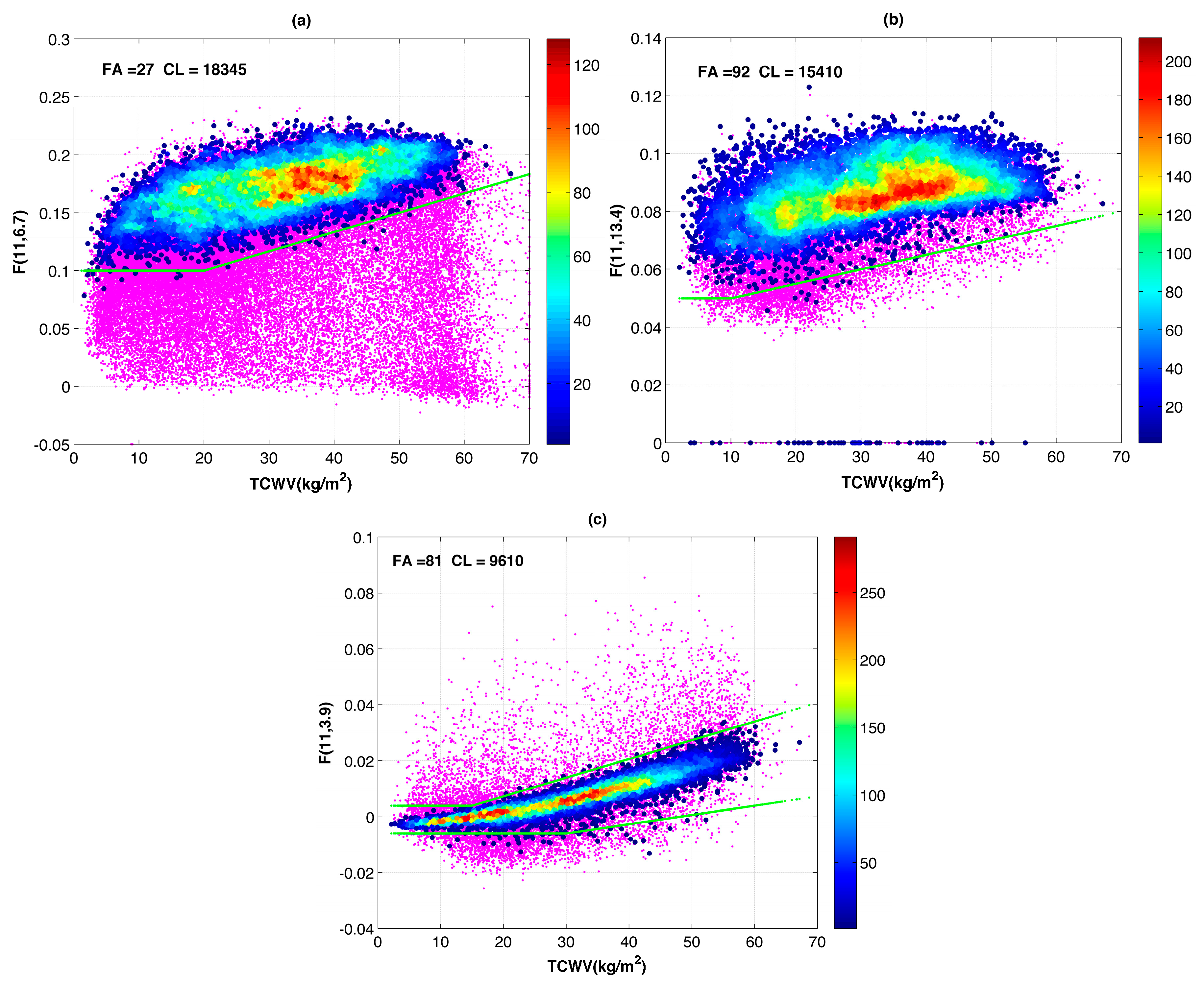
where, $T_a^m$ stands for the measured brightness temperature of MODIS-A for channel “a”. We found that the calculated coefficients using GOES-13 for TCWV dependent spectral differences between 3.9, 11, and 13.4 μm channels work reasonably well for MODIS, as we reported in earlier work [16] regarding the advantage of normalized spectral differences. To demonstrate this, we progressively separate the matchups of August 2014 into two classes, as ‘Selected’ and ‘Discarded’, employing Equations (6)–(8) sequentially. Before the first test, all data were assigned to the ‘Selected’ class (note that the implementation of real images will be different, where all tests should be applied at the individual pixel level to determine the status of ‘Cloudy’ or ‘Cloud-free’). First, we plot the normalized spectral differences of 6.7 and 11 μm channels with TCWV using coefficients of GOES-13 for separating the cloudy and cloud-free classes (green line), which is shown in Figure 1a. The density plot of cloud-free pixels according to the experimental filter (EXF), which is described in our earlier publication [16], is superimposed. EXF is a tool to detect the cloud-free pixels, and the condition is $abs(s_b-s_g-rt{v}_{3.9}$) < 1, where $rt{v}_{3.9} = \frac{T_{3.9}^m-T_{3.9}^s}{K_{SST}^{3.9}}$ and $T_a^s$ stands for the simulated brightness temperature of MODIS-A for channel “a”. Note that this is only used to verify the cloud detection scheme.

Figure 1a demonstrates that the first cloud test eliminates 10,517 pixels, at the cost of only 27 good measurements. As we mentioned in our earlier publication, the main motive is to use a flexible threshold to discard only pixels which have a high expectation of cloudiness, and the results show exactly this. A total of 18,345 cloudy pixels remain in the ‘Selected’ class underneath the density plot of cloud-free pixels (according to EXF). The pixels considered in the second test are those that remain in the ‘Selected’ class after the first test. Similarly, Figure 1b shows that 3027 pixels are discarded, including 92 good measurements, after applying the second test, i.e., 15,410 cloudy pixels still remain in the ‘Selected’ class. A further 5881 pixels, including 81 good measurements, are discarded, leaving 9610 cloudy pixels in the ‘Selected’ class after applying Equation (8), as shown in Figure 1c.

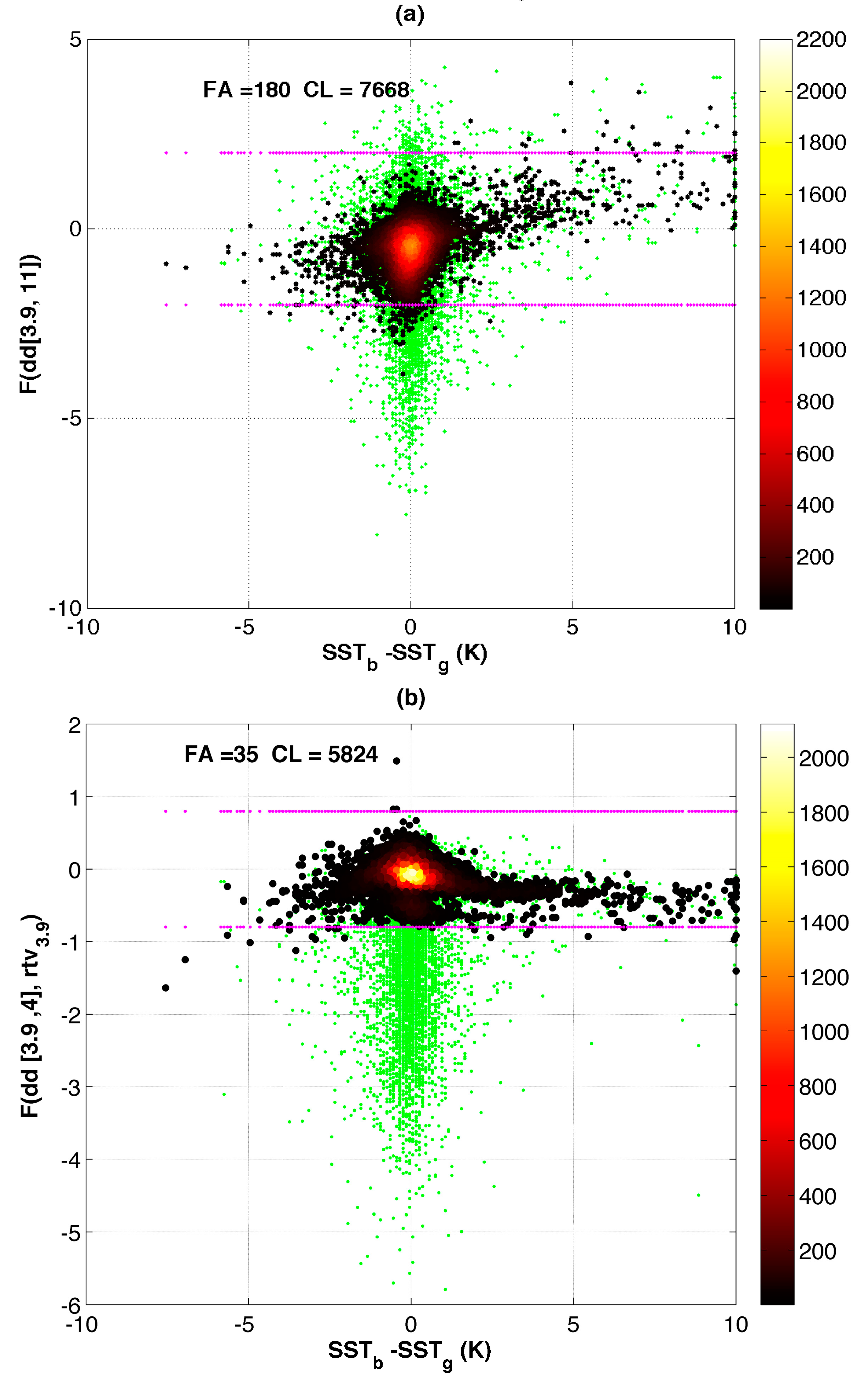
As we mentioned in our earlier publication [16], spectral differences alone cannot completely remove all cloudy pixels, and an additional RT-based double-difference (measurement minus observation) 3.9 minus 11 μm test was implemented. Applying this test to MODIS data removes a significant number of good measurements when the absolute value of (SST_b-SST_g) is close to zero, as shown in Figure 2a. As more channels are available in MODIS, we explore alternate tests to improve the performance of CEM. Empirically, we develop an alternative double-differences test to preserve most of these earlier discarded pixels. The test is the double-differences between the channels of 3.9 and 4.0 μm (dd3_4), which was not possible to implement previously, due to absence of the 4.0 μm channel in GOES-13.

$$abs\left(dd\left[\mathrm{3.9,4}\right]\right)< 0.8*(0.1+\frac{\max \left(rt{v}_{3.9}, 2\right)}{10}+\frac{\min \left(rt{v}_{3.9}, -1\right)}{3})$$

(9)

Figure 2a,b shows that 145 good measurements can be saved and additional 1844 cloudy pixels can be discarded by using the new double difference test instead of the previous one. The double difference method is a well known means for minimizing the influence of the forward model error.

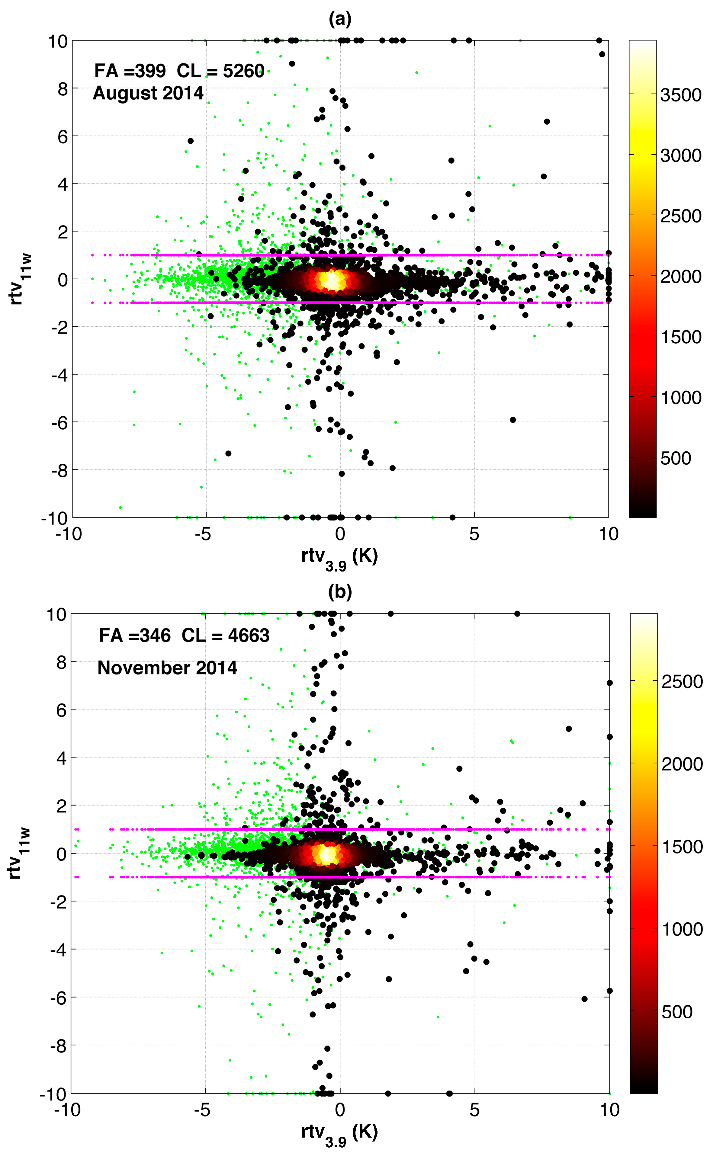
An RT-based water vapor threshold filter ($rt{v}_{11w}$) is applied for the whole dataset, as reported in our earlier publication [16], and eliminates 963 cloudy pixels at the cost of 399 good measurements, as shown in Figure 3a. This is based on a single-channel retrieval of TCWV from the 11 μm measurement (rtv_11w), using a linear assumption, and rtv_3.9 as we described earlier:

$$rt{v}_{11w}=\frac{T_{11}^m-T_{11}^s-K_{sst}^{11}rt{v}_{3.9}}{K_{TCWV}^{11}}$$

(10)

Here, we modify the threshold of this test and restrict it to a particular region where the value of rtv_3.9 is less than −2 K (bearing in mind that retrievals are deltas from the initial guess SST) and pixels are discarded if the absolute value of $rt{v}_{11w}$ is greater than 0.1 (~10% variability of TCWV). To give more confidence in our cloud detection, we also present the results from a winter month of November 2014 after applying all tests (Figure 3b).

We retain our previous three-by-three spatial homogeneity filter [16] to remove pixels affected by cold fractional clouds. The BT values of the eight pixels surrounding the target pixel are compared. We have employed two different threshold conditions for the adjacent nine measurements: (a) the “maximum minus minimum” of these measurements should be less than 5 K (which is a substantially relaxed filter cf. other methods); (b) the value of the target pixel must be within 0.8 K of the maximum value.

4. Comparative SST Retrievals

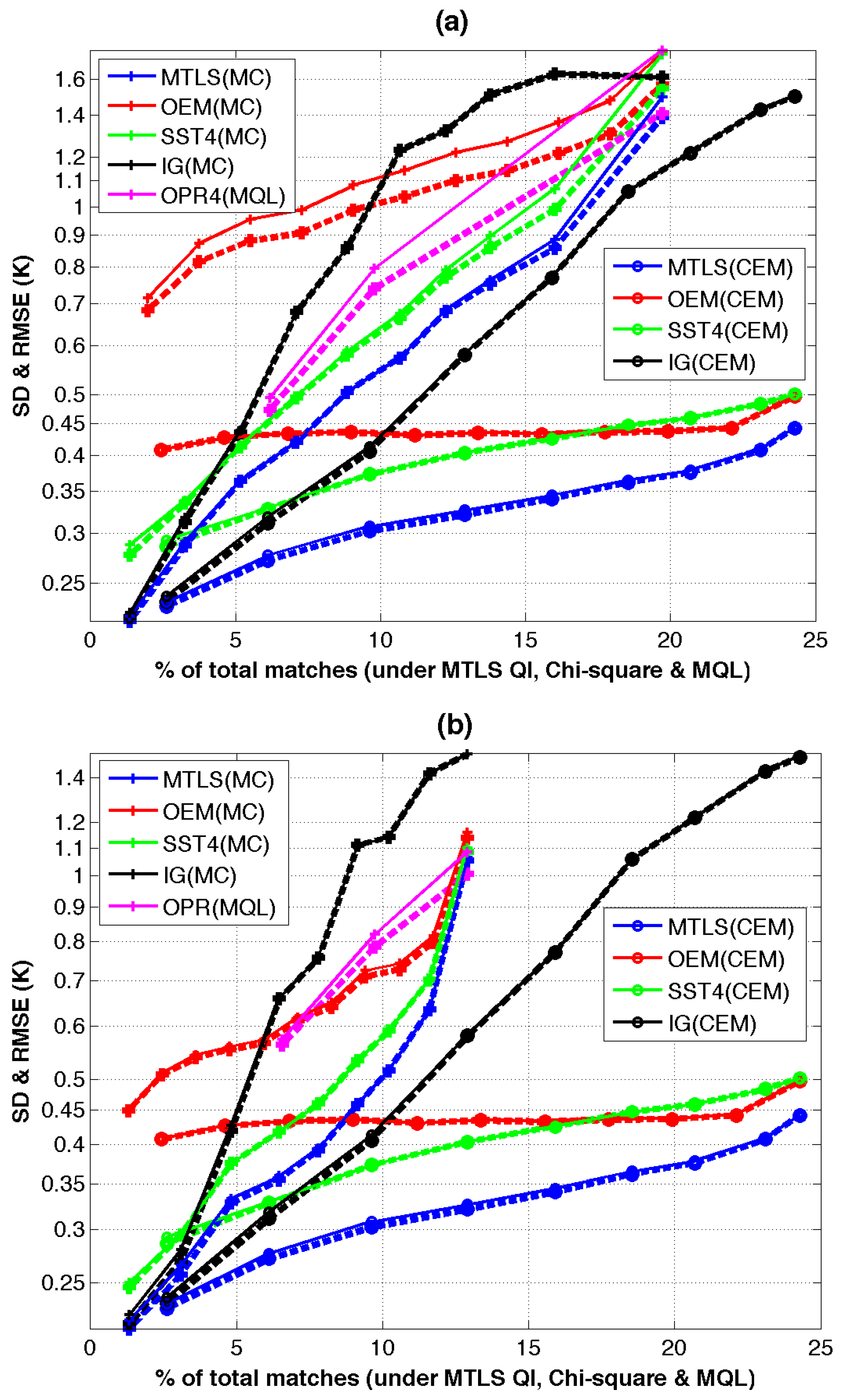
We confine detailed discussion to results for the month of September 2014 in this paper, and time series results will be discussed in a future publication. The retrieval errors for three different methods and two different cloud detection schemes are shown Figure 4. The errors in SST retrievals are shown in Figure 4 using two different metrics: (a) root mean square error (RMSE), and (b) standard deviation (SD). RMSEs are plotted on top of the SDs—when the lines merge (i.e., the dashed SD line is not visible) the systematic error component of RMSE is negligible. The error (RMSE and SD) of MTLS, SST4 and IG are ordered with respect to increasing MTLS QI, while OEM results are ordered with respect to chi-square, and OPR with respect to MQL. Although we assume that the cloud-free pixels (available at http://modis-atmos.gsfc.nasa.gov/MOD35_L2/) can be obtained if the subset of the pixels of MQL ≥ 3 is considered, it turns out that MODIS nighttime L2P files generally contain are two different MQL fields for two distinct operational MODIS products (short-wave and long-wave). Two subsets of pixels (MQL ≥ 3) for two different products are significantly different. It is not an unreasonable expectation that, first, the cloudy pixels are discarded using MC, and then the SST quality level is assigned according to the performance of the retrieval algorithm in operation. However, since the subsets for the cloud- free pixels from the two different products are so different, we will consider the cloud-free pixels of MC for these two different operational products separately. More discussion on this is in Section 5.

The number of cloud-free pixels for our new cloud detection is modestly higher (difference is only 10%–15%) than for OPR4, but the RMSE of the operational shortwave SST (MQL ≥ 3) is ~1.8 K, which is four times higher than the RMSE of MTLS (0.38 K) for the equivalent coverage of ~20%, as shown in Figure 4a. Note that there is also significant bias in the OPR4 data with MQL ≥ 3, since the SD is less (1.4 K), implying a bias of order 1 K. The RMSE of short-wave MODIS SSTs is ~0.5 K for the highest MQL = 5, giving coverage of ~6%, while the RMSE of MTLS is ~0.4 K, i.e., lower than OPR4 at MQL = 5, with a data coverage of ~23%. This implies a four-fold information gain using MTLS + CEM over OPR4 with the MODIS cloud/quality flagging. The RMSE of short-wave operational MODIS SSTs is ~0.8 K at MQL = 4 for a data coverage of ~10%, while the RMSE of MTLS for the same data coverage (but different subset of pixels) using our CEM is 0.3 K. Apart from this, MTLS has an additional advantage that it can calculate retrieval error at the individual pixel level. MTLS QI can improve the result (blue circle) from 0.4 K for 23% data coverage to 0.25 K for a data coverage of ~5%, as shown in Figure 4a. The MTLS QI can also be used to identify the higher quality SST4 observations, where the RMSE of ~0.5 K (circle green) for 23% matches (i.e., using our CEM) can be reduced to 0.32 K for the best 5% of matches. MTLS QI also shows an excellent performance for the retrieval of MTLS (blue, plus) and SST4 (green, plus) for data screened using the MODIS cloud mask. As neither SST4 retrieval nor MC use a forward model, this implies that the basic premise of MTLS QI is not sensitive to the choice of forward model.

The RMSE curve of OPR4 in Figure 4a against MQL is comparable with the RMSE curve of SST4 against MTLS QI, where coefficients are calculated offline. A significant improvement of RMSE of SST4, which regression based retrieval, under CEM from 1.6 K to 0.47 K for the data coverage of 20% as compared to the same of MC, gives us confidence on the superiority of CEM over MC. As the curves of the RMSE of SST4 and MTLS are almost parallel under MTLS QI with a relatively small difference of 0.050–0.1 K for both cloud masks, this may raise a question about the justification for the forward model run, which is computationally expensive. However, the improved QIs for SST4 from ~1.6 K to ~0.3 K under MC and from 0.5 K to ~0.3 K under CEM cannot be made without the MTLS QI (based on forward model calculation), and the forward model run is an essential component of the CEM as well.

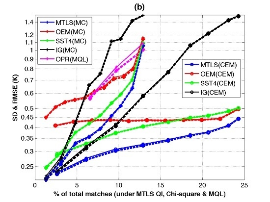
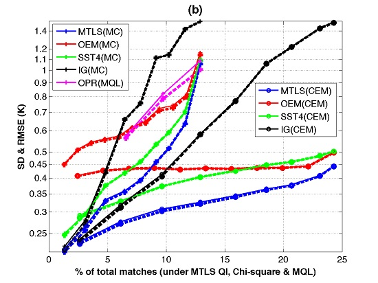
The new cloud detection scheme classifies ~2 times as many pixels as cloud-free (i.e., able to obtain a good SST estimate) compared to the standard MODIS cloud algorithm, according to the MQL ≥ 3 of the long-wave operational MODIS SST product (Figure 4b). Note, however, that, the standard MODIS cloud-free pixels are not simply a subset of our set. Figure 4b shows that the RMSE of OPR for MQL of 5 is ~0.57 K and only comprise ~6.5% of the total number of matchups. On the other hand, the new cloud detection classifies cloud free pixels are ~23% (except last bin), with RMSE of MTLS of ~0.4 K. This represents approximately 3–4 times the information gain in terms of low error and high data coverage using the combination of CEM and MTLS. The data coverage of operational MODIS SSTs can be increased up to ~13% by decreasing MQL of 3 (long-wave), but with a concomitant increase of RMSE to ~1.1 K. The information gain for CEM+MTLS is ~3 times even if we consider a threshold of cloud at MQL ≥ 3. It is also observed from this figure that the IG error for the whole cloud-free dataset using CEM is comparable to that for the group of MODIS cloud-free (MQL ≥ 3) pixels, which eliminates the possibility that CEM is only selecting the pixels with SSTs close to the IG.

The retrieval errors for all retrievals are reduced with the new cloud detection. The RMSE of MTLS reduces from 0.65 K to 0.4 K (except the last bin, which is reserved for “bad” retrievals, as described earlier), similarly OEM also reduces from ~1.6 K (according to short-wave MQL) and 1.1 K (according long-wave MQL) to 0.5 K (including last bin, as chi-square approach unable to provide additional cloud mask information at solution time). Some noteworthy comparison results between OPR and SST4 are: (a) RMSE values for both SST4 and OPR are similar for quality level of 3 but the RMSE of SST4 is 0.42 K (30% reduction from the value of OPR) using the MTLS QI for a similar number of pixels as quality level 5 data (i.e., ~6.5%, vertical comparison); and (b) for the same RMSE as MQL = 5 (0.42 K), the data coverage increases from 6.5% to ~10% when using the MTLS QI.

Both MTLS and OEM solutions are based on the same physical model, but the results are significantly different. The RMSE values of MTLS and OEM under CEM for the whole cloud-free dataset are 0.44 K and 0.5 K respectively, which are fairly comparable, however, the RMSE of OEM (~0.43) is 40% higher cf. MTLS (~0.31) for the best ~10% of data. MTLS solves the problem deterministically, deriving the equation at the individual pixel level, whereas OEM solves the problem stochastically, using properties (the error covariances) from a set of measurements. Thus, OEM-retrieved products always contains some ambiguity with respect to individual pixel level quality. Furthermore, it involves significant risk to develop science relying on a fundamental flaw, where error is treated as definite information, even though one may produce best retrieval results (statistical sense) for a particular month of match-ups as compared to other methods by tuning the used error values as input to OEM. The main difficulty in implementing OEM operationally is that it requires accurate a priori and error covariance matrices, which are very difficult to estimate for individual retrieval conditions. Perhaps the most interesting result is that the a priori error is less than the posteriori error for 30%~40% OEM retrievals under both cloud schemes, i.e., the OEM solution degrades the initial guess, whereas this never happens for the MTLS solution. The OEM error is always higher than that of SST4 under both cloud schemes of MC. Even though our modified CEM discards some pixels due to forward model error and only use infrared channels, the data coverage is still improved by a factor of ~2 as compared to the current MODIS cloud algorithm.

The good SST4 retrieval results under CEM confirm that the consistency is not exclusively between the CEM and MTLS, since the SST4 does not use a forward model. However, we extend the comparison study to the operational MODIS cloud regime (both short-wave and long-wave) to gain more confidence in the method. The MTLS solution still provides superior results cf. other retrievals when using the standard MODIS cloud mask (MQL ≥ 3). It is noteworthy to mentioned that the RMSE of MTLS (under MTLS QI) using the long-wave operational MODIS cloud mask is still ~0.36 K for the best 6.5% of all data, which is the equivalent number of match-ups for OPR at the highest MQL = 5. Similar results are also found in the short-wave MC. In Figure 4b, the RMSE of MTLS and OEM for ~13% of total match-ups of MODIS cloud (MQL ≥ 3) are close; however, the RMSE of OEM (~0.6) is 50% higher cf. MTLS for the best ~6.5% of data. These are similar differences to those mentioned earlier using CEM, which confirms that the QI of MTLS is superior compared to the chi-square of OEM. Again, the same argument can be made that the relative failure of the chi-square based QI of OEM is due to its reliance on stochastic information (error covariances) in the solution, thus there is less confidence in both the retrieval at the individual pixel and its quality indexing.

5. Verifications of Cloud Schemes

The last bin of MTLS, which is intended as an extra cloud filtering step, and chi-square-based evaluation of the last bin under the MODIS cloud, both show a sharp reduction in retrieval error for discarding relatively few pixels. The RMSE of SST4 and MTLS have sharply reduced under both MC for the last bin using MTLS QI in Figure 4a,b. This implies that there is significant cloud leakage in the MODIS cloud. Thus, we have conducted a simple test using pixels with collocated buoys to verify the performance of the cloud detection technique using EXF. Detailed discussion of this experimental filter can be found in our earlier publication [16]. 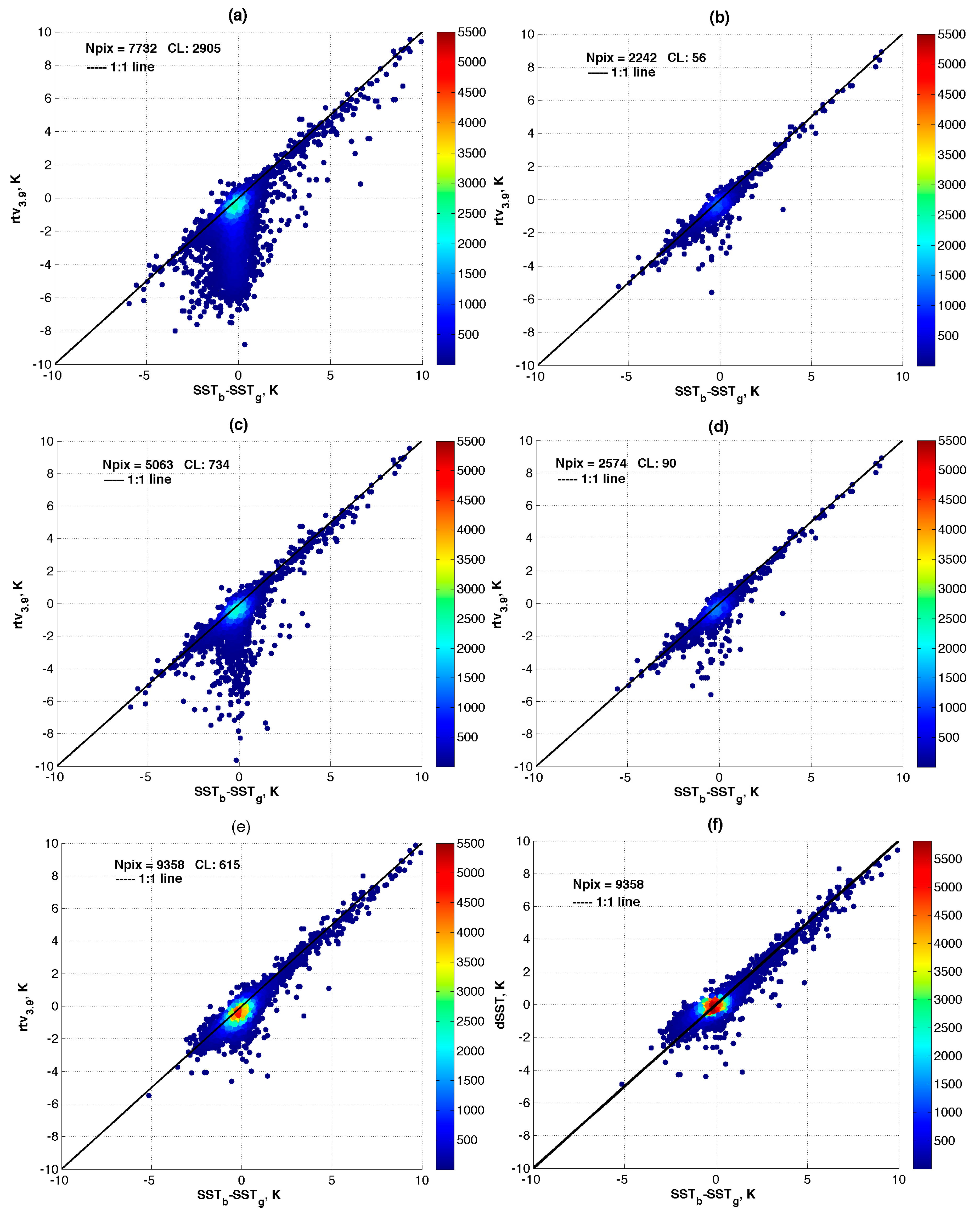The BT differences (“modeled minus observed” BTs in 3.9 μm) for each pixel are divided by the Jacobian (SST) values to transform them from measurement space to state space and enable a direct comparison with “IG minus Buoy” (this is essentially a single-channel SST retrieval using the 3.9 μm channel, and since the effect of water vapor on the 3.9 μm channel is fairly modest, the SST Jacobian is adequate for this purpose of normalization). Provided that the pixels are cloud-free, the points should closely follow a 1:1 ratio. Figure 5 shows the single channel retrieval of 3.9 μm for the subset of pixels coming from (a) MC (MQL ≥ 3 of the short-wave SST product); (b) MQL = 5 (again shortwave SST); (c) MC (MQL ≥ 3 of the long-wave SST product); (d) MQL = 5 (again long-wave SST), and (e) CEM against “IG minus Buoy”.

Figure 5 shows the density plot of rtv_3.9 with the distance between the true and IG SST under two different cloud detection schemes. There are significant cloud leakages for the MODIS cloud for MQL ≥ 3 (Figure 5a,c), evidenced by the large number of points far below (e.g., <−5 K) the 1:1 line, especially where the buoy temperature is close to the initial guess. The concentration of points in this region is expected to be high, since in situ data are typically used in the construction of the IG (in this case, the NCEP SST). Although the data coverage for MC (7732 shortwave) is below and for MC (5063 longwave is far below than that of the new cloud detection scheme (9358 Figure 5c), it is also worse in terms of retrieval accuracy for this month. The cloud leakage significantly reduces for MQL = 5 for the MODIS cloud (Figure 5b,d), but it is still inferior to the new cloud detection scheme (Figure 5e) and, at the same time, the data coverage (2242 and 2574) is reduced to approximately one fourth, compared to the new cloud detection.

The cloud leakage (CL) according to EXF is 2905 points for the OPR4 product, whereas the number is only 754 for the OPR product. The increased data coverage in short-wave operational SSTs at MQL ≥ 3 (as shown in Figure 4a), as compared to the long-wave (Figure 4b), is mostly caused by the inclusion of cloud-contaminated pixels. The reason for the substantial difference in QL = 3 data between the long-wave and short-wave SST products in MODIS is not immediately obvious, because the tests are essentially the same (see http://oceancolor.gsfc.nasa.gov/cms/atbd/sst/ doc/html/flag.html). However, one possibility is that the spatial uniformity test degrades all long-wave MODIS SST data by one quality level (see footnote 2 of “Minimum Quality Level” table in above link) but this does not appear to be applied to the shortwave MODIS SST product. Thus, long-wave MODIS SST data, which were originally GHRSST QL = 3, may have been degraded to QL = 2 and, therefore, not considered in our analysis. Recommended guidance for MODIS GHRSST data is actually to only use QL 4 and 5 (Kilpatrick, pers. comm.), which reduces the coverage of OPR4 from ~20% to just under 10%, and OPR from ~13% to also just under 10%. The inclusion of QL3 data which, according to general GHRSST guidelines, ought to be usable (if potentially suspect) is justified here because a large part of this analysis is investigating the partition of data by quality level and the effects of cloud contamination. Finally, it should be noted that CL of 615 out of 9358 (~7%) points still exist for CEM, as shown in Figure 5e, but very few of them are more than 2 K. However, a further improvement of CEM is required.

It is observed from all plots in Figure 5a–e that rtv_3.9 for the majority of pixels do not lie exactly on the 1:1 line for either cloud detection scheme. This bias may be due to the effect of TCWV on the BT of 3.9 μm, which is considered to be zero (i.e., exactly correct) in EXF. This explanation is given further weight by the innovation plot of MTLS under CEM in Figure 5f, which shows essentially no bias for the peak of the distribution, since it has the advantage of allowing compensation for water vapor in its retrieval space cf. the simple single-channel SST retrieval. MTLS solutions follow a 1:1 ratio, even when SST_b is 10 K higher than SST_g in Figure 5f, which also confirms that the influence of NWP data and CRTM is minimal, even though we use the RT simulation in the cloud detection scheme.

6. Conclusions

This study shows that the performance of the deterministic inverse method of MTLS is better than the other methods under consideration when using different cloud detection schemes, and copes well with various operational problems. The additional cloud detection and quality flagging using the analytic error calculation at the solution time of MTLS are fully objective and results display compliance with in situ validation. On the other hand, the quality flagging using chi-squared estimation displays ambiguous qualities. GOES-13-derived coefficients for cloud detection using normalized spectral differences with functional dependence on, e.g., TCWV, also work well for MODIS, which implies that a physically-based model is a better choice than coefficients derived purely from stochastic properties of observed, e.g., brightness, temperatures.

The operational SST products available from the GHRSST website do not appear to be optimal in terms of quality and data coverage. The MTLS algorithm, in conjunction with the new cloud detection scheme, as well as the quality indexing at the individual pixel level, should improve the situation. MODIS-derived SSTs have many applications in atmospheric and oceanic studies, and with more than one and a half decades of continuous data availability, they form a tremendously important part of the geophysical record. An increase of 3~4 times the information content, as presented here, compared to the operational available MODIS SSTs, should open up a new horizon in a variety of geophysical applications.