Registration of Airborne LiDAR Point Clouds by Matching the Linear Plane Features of Building Roof Facets

Abstract

This paper presents a new approach for the registration of airborne LiDAR point clouds by finding and matching corresponding linear plane features. Linear plane features are a type of common feature in an urban area and are convenient for obtaining feature parameters from point clouds. Using such linear feature parameters, the 3D rigid body coordination transformation model is adopted to register the point clouds from different trajectories. The approach is composed of three steps. In the first step, an OpenStreetMap-aided method is applied to select simply-structured roof pairs as the corresponding roof facets for the registration. In the second step, the normal vectors of the selected roof facets are calculated and input into an over-determined observation system to estimate the registration parameters. In the third step, the registration is be carried out by using these parameters. A case dataset with a two trajectory point cloud was selected to verify the proposed method. To evaluate the accuracy of the point cloud after registration, 40 checkpoints were manually selected; the results of the evaluation show that the general accuracy is 0.96 m, which is approximately 1.6 times the point cloud resolution. Furthermore, two overlap zones were selected to measure the surface-difference between the two trajectories. According to the analysis results, the average surface-distance is approximately 0.045–0.129 m.

1. Introduction

Registration is one of essential preprocesses for the data analysis of point clouds acquired by a laser scanner because the data can be obtained by using different platforms e.g., terrestrial or mobile laser scanning from the ground or airborne laser scanning from airplanes. The point clouds captured by different platforms have good complementarity with the data registration. Different scan stations or trajectories lead to misalignment of a point cloud. The co-referenced point cloud is highly referenced in 3D modeling, surface reconstruction, and information extraction [1,2,3].

The most common approach for point cloud registration in the existing research literature involves artificial targets, such as reflective balls. These targets are regarded as corresponding objects in two different data sources and then apply coordinate transformation models, such as the Bursa model and the 3D rigid body model. In this type of method, the 3D rigid body model is usually assumed, and the scale parameter between two datasets is ignored due to the direct measurement of laser scanning. The method is widely used in terrestrial laser scanning, and many software packages support the automatic extraction of the reflective balls from the point cloud and calculate the coordinates of the ball center. The spatial distributions of the artificial targets are important for model parameter calculation and accuracy evaluation [4].

However, artificial targets can hardly be deployed in the measurement campaign of mobile and airborne laser scanning for several reasons. First, applying artificial targets within the measurement field carries a high cost in terms of labor and money because the field is normally large. Second, the density of a point cloud is lower than that of terrestrial laser scanning, especially in airborne laser scanning cases. Therefore, it is difficult to identify target balls from an airborne point cloud.

To co-reference the point cloud without using artificial targets, some automatic registration approaches have been proposed by different researchers. Among them, the ICP (Iterative Closest Point) based algorithm [5] is one of the most popular methods.

The ICP algorithm is sometimes applied to the dataset with different reference systems and aligned in a pre-process. In addition, it is often used to match two datasets with overlapping areas and is usually captured by the same type of platform. The pre-alignment operation is applied to reduce the difference between two datasets and is usually conducted manually. Pre-alignment also provides the rough registration results for precise matching. Then, an iterative refinement technique is used by identifying corresponding points and estimating the best relationship between two datasets. During the relationship estimation, an error matrix is established to evaluate the error between corresponding points.

Based on the basic ICP algorithm, some extensions and additional conditions were developed to increase the robustness and convergence, as well as to improve the computational efficiency and performance. For example, RANSAC (random sample consensus) [6] or LMS (least median of squares estimators) [7] were proposed and applied for data registration.

Another category of approaches for point cloud registration is a geometric-feature based method. Point features, line features, plane features, curvature feature, and terrain should be first extracted and then used to co-reference the different sources of the point cloud. The geometric feature-based algorithms are usually performed semi-automatically because the correspondence among features are normally manually identified. For example, Cheng et al. [8] and Zhong et al. [9] used corner points of buildings and proposed semi-automatic method for point cloud registration. [10] proposed a semi-automatic method using feature line and feature polygon to matching the point cloud captured from terrestrial and airborne laser scanning systems under the assumption that the rotation angles between X and Y are zero, which is difficult to satisfy in a real situation. However, this method can be used to register a point cloud with low overlap zones. Li and Guskov [11] proposed a method to detect a set of salient feature points and use a significance vector as an approximate invariant. Then, the feature sets were used to obtain the alignment between two datasets. Similar to [11], Alba et al. [12] and Weinmann et al. [13] used line and plane features extracted from a point cloud to obtain accurate alignment results. Variation in the curvature is a special feature used for point cloud registration [14]. The normal vector and the curvature from an unorganized point cloud should be calculated in advance [15]. Hansen et al. [16] used the 3D line features derived from both terrestrial and airborne point clouds registration. Then, a two-step registration method is performed. According to their research, this method will be easily affected by noise. A recent publication [17] proposed a registration method based on a hierarchical and coarse-fine strategy to co-reference a point cloud from airborne and vehicle platforms. According to their analysis, this method can achieve an average accuracy of approximately 0.4 m.

Curvature features [18] are other types of features used for registration. The curvature parameter for each point is computed from different datasets, and the initial feature points are selected by maximum local curvature variations. Last, the Hausdorff distance is used to obtain accurate matching points and to estimate the rotation and translation matrix.

Some other types of data sources are also used to aid point cloud registration, such as imagery and topographic maps. Dold and Brenner [19] proposed an autonomous method based on planar patches automatically extracted from point clouds and imagery. Wu et al. [20] proposed a method using a topographic map as reference data and transferred a point cloud captured from both terrestrial and airborne laser scanning systems to the local coordinate system. During this research, the building feature lines and control points of topographic map were selected for feature based registration. Supplementary data sources usually imports a local or special reference coordinate system; therefore, this type of method is helpful for further integration and application. [21] proposed a 3D building histrogram to represent the complexity of buildings and uses SD (block distance between the two histograms) and ZLB (z-value of the largest class in the 3D histogram) as the indices to describe each building roof and co-register the multi-layer and single-layer buildings. Yu et al. [22] extracted the semantic features (such as facades, poles, cars) from city environment and used the ICP algorithm to align the point cloud from Google Street View cars.

This paper proposes a novel approach for the registration of airborne point cloud data sets by using linear polygon features of building roofs. In the first step, the methods developed in previous research [23] will be applied to extract buildings and identify buildings with gabbled and hipped roofs in the two datasets, respectively. The buildings identified with the same building footprint on OpenStreetMap (OSM) are, therefore, the corresponding buildings in the subsequent process. Next, the normal vectors are calculated for every simple roof facet of the corresponding buildings. These normal vectors will be used to calculate the transformation model between the two datasets; therefore, the least squares (LS) method will be deployed to solve the observation system with redundant feature-pairs.

The rest of the paper is organized as follows. Section 2 introduces the proposed method, including the principles of the registration method in this paper, the flowchart of the proposed method, and the mathematical models. In Section 3, the study area, as well as the experimental results and the accuracy evaluation results, is presented. Section 4 summarizes the proposed method and discusses the limitations of the proposed method.

2. Point Cloud Registration by Matching Plane Features of Building Roof Facets

To describe the two dataset used in this paper, we discuss two point cloud datasets to be registered as ${\left(\begin{array}{ccc}X& Y& Z\end{array}\right)}_{C1}$ and ${\left(\begin{array}{ccc}X& Y& Z\end{array}\right)}_{C2}$, where the subscript C1 and C2, respectively, are used to separate the datasets. The purpose of this paper is to find a proper transformation parameter to reduce the difference between two datasets.

In this paper, the rigid body model is chosen for point cloud transformation, whereas the steps of the other models (e.g., Bursa model) for registration are similar to the rigid body model. The rigid body model uses a 3D shift vector and a 3D rotation matrix to describe the relationship between two datasets. The mathematical model is described as:

$${\left(\begin{array}{c}X\\ Y\\ Z\end{array}\right)}_{\mathrm{C}2}=\left(\begin{array}{c}\Delta x\\ \Delta y\\ \Delta z\end{array}\right)+R\left(\mathsf{\alpha },\mathsf{\beta },\mathsf{\gamma }\right){\left(\begin{array}{c}X\\ Y\\ Z\end{array}\right)}_{\mathrm{C}1}$$

(1)

where $\left(\Delta x,\Delta y,\Delta z\right)$ is the 3D translation vector, and $R\left(\mathsf{\alpha },\mathsf{\beta },\mathsf{\gamma }\right)$ is the 3D rotation matrix that is defined by the axis angles $\left(\mathsf{\alpha },\mathsf{\beta },\mathsf{\gamma }\right)$ between C1 and C2. Therefore, computing the proper 3D translation vector and the 3D rotation matrix is the essence of registration, and it determines the accuracy of registration.

2.1. Principle and Flowchart of Proposed Method

For a typical coordinate transformation model, 3D points are usually used to calculate the 3D translation vector and the 3D rotation matrix of the rigid model. After selecting several 3D point pairs from different datasets, a least square adjustment processing is applied to compute the parameters. However, laser scanners use a huge number of points to describe a certain object. The accurate point-to-point relationship is difficult to follow. Therefore, in this paper, the linear polygonal features of buildings, instead of 3D point-pairs, are selected to calculate the coordinate transformation parameters. 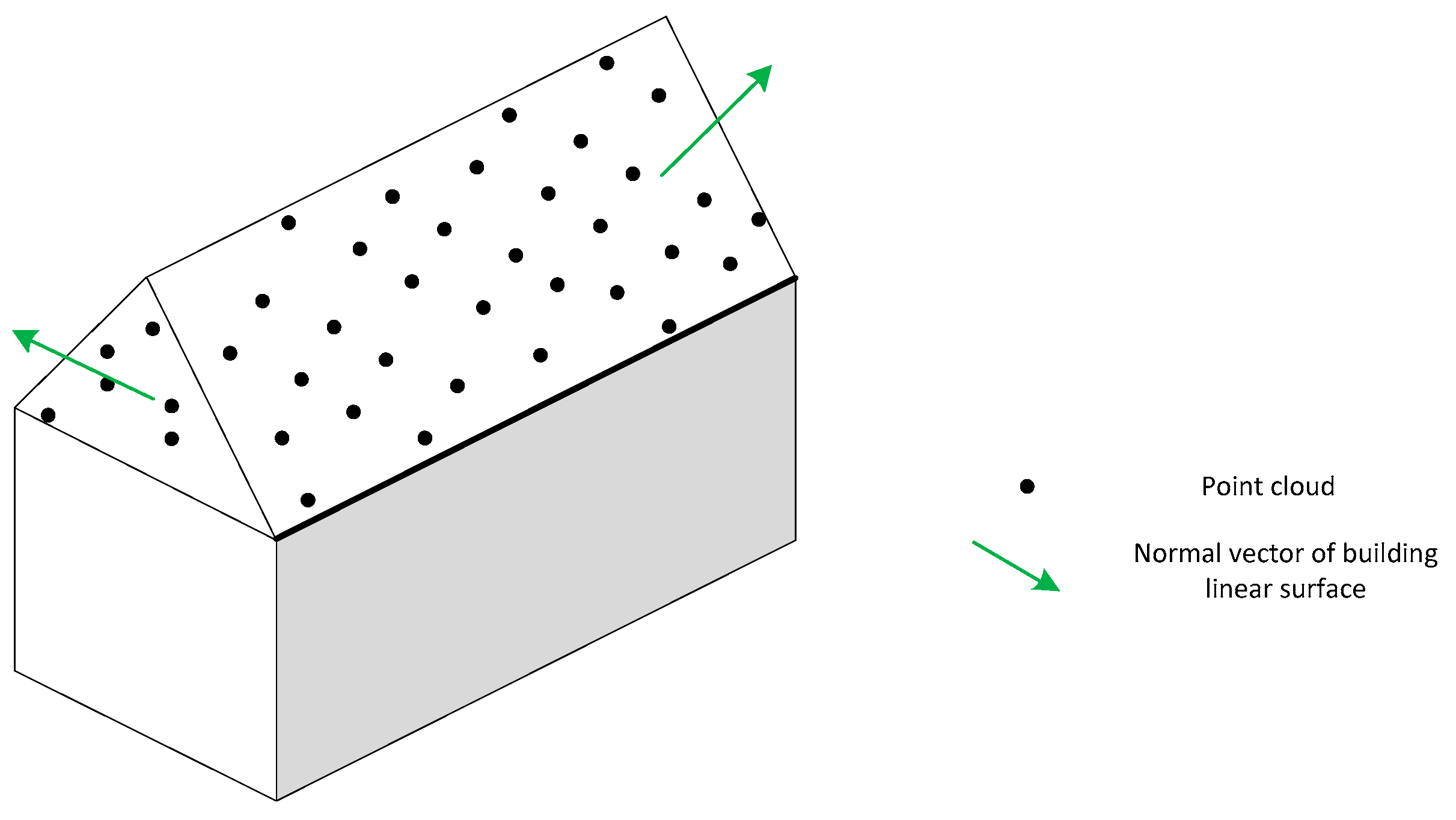Figure 1 shows the point cloud of a building roof and its corresponding normal vectors.

An airborne laser scanner obtains the reflected laser beams to compute the coordinate of surface of terrain objects. In an urban area, the surface points of building are the main components of an urban point cloud. Meanwhile, linear polygonal roof features are the main features of a building; such features can be easily found and the feature parameter can be easily obtained to perform airborne point cloud registration.

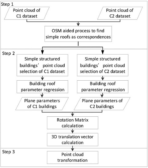
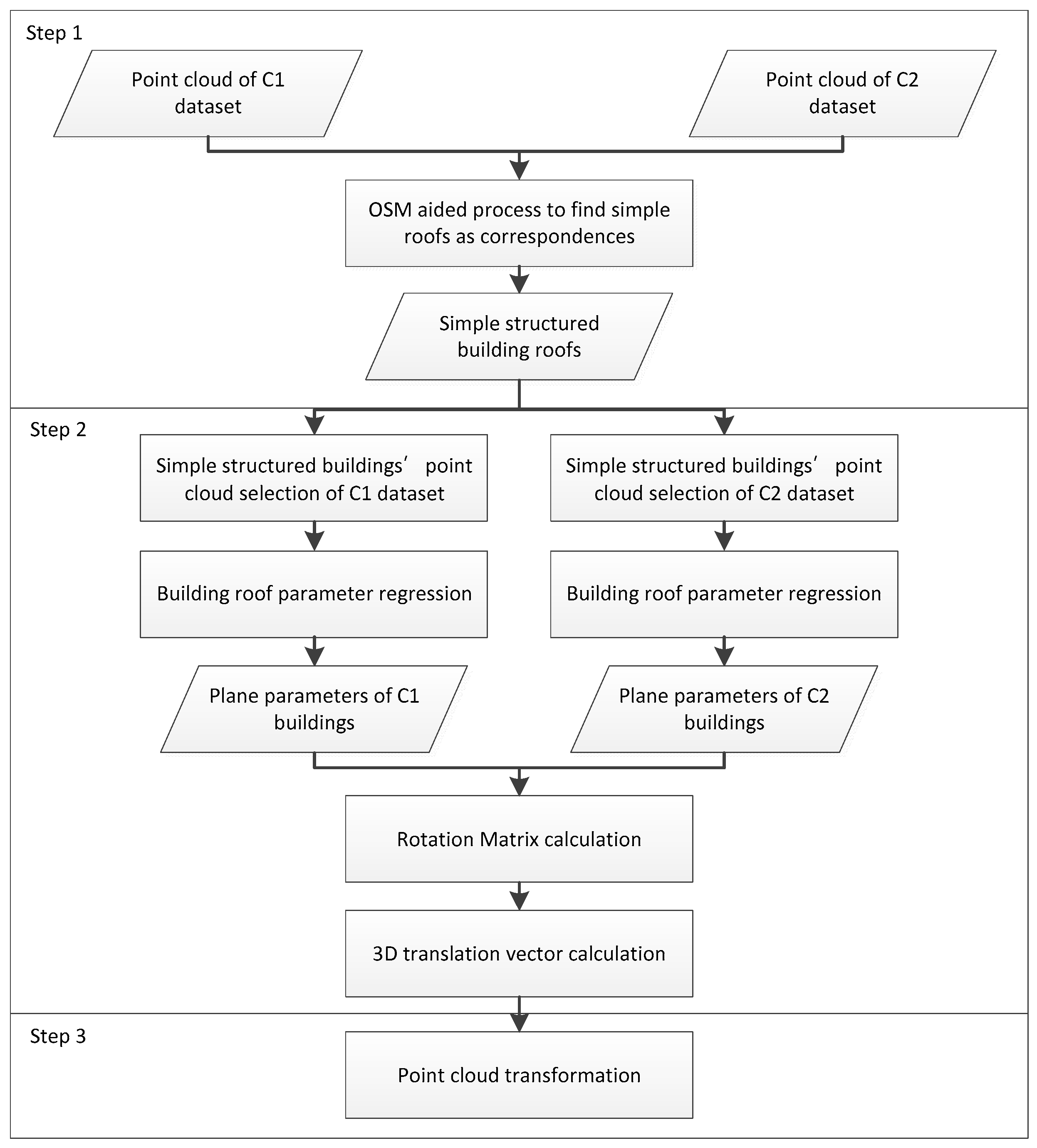
Figure 2 illustrates the process of the registration. After the simple buildings (with simply structured roofs) are extracted, the vectors of the roof facets are calculated. The vectors of the corresponding roof facets can then be used to establish an observation equation system to estimate the transformation between the two datasets. The flowchart can be divided into two main parts.

First, the point clouds of the building roofs are extracted from the two LiDAR datasets. This extraction is achieved by using an OSM aided approach presented in [23]. In the next step, the point clouds segmentation will be conducted by adapting the method of ridge-based hierarchical decomposition. Specifically, a roof will be selected for the subsequent process when only less than one ridge can be detected. In other words, only simple structured roofs, such as gabble, hipped, or flat roofs, will be selected for the registration of the two datasets. Then, the point clouds of simple structured buildings are automatically selected based on the roofs.

The second part is the registration parameter calculation and will be divided into two steps: the rotation matrix calculation and the 3D translation vector calculation. The detailed steps and functions for rotation matrix and 3D translation vector calculation will be introduced in Section 2.3.

2.2. Calculating the Normal Vectors of Building Roof Facets

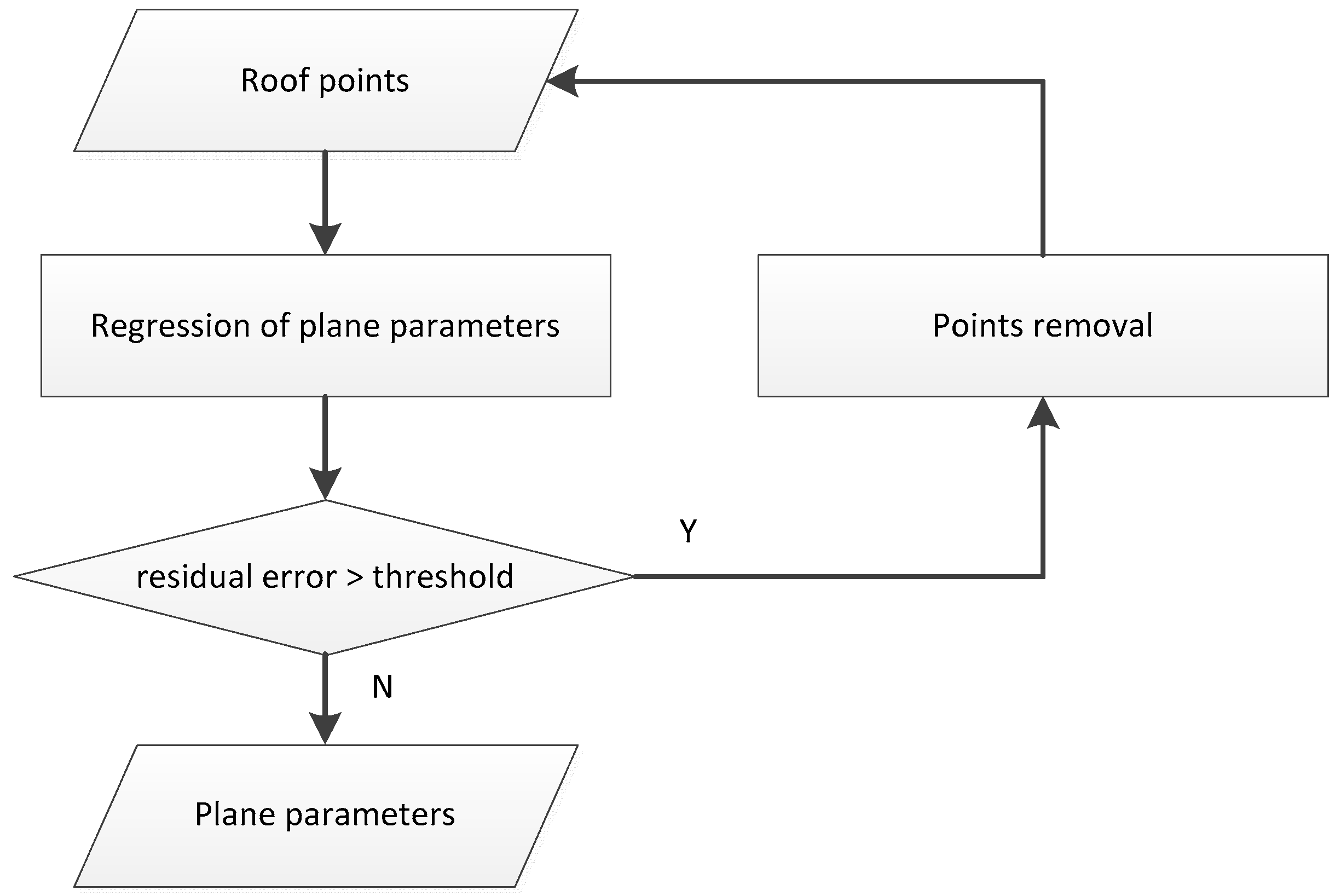
A plane-fit program is performed after the building roof points are separated. The detailed steps of the plane parameter extraction are shown in Figure 3.

After the roof points are extracted from the original point cloud, a plane regression algorithm is applied to the roof points and the plane parameters (see A, B, C, and D in Equation (2)) are obtained. Several mathematical forms can be used to represent the plane equation.

$$AX+BY+CZ=D$$

(2)

where (A, B, C) represent the unit normal vector of the plane, and D denotes the distance between origin to the regressed plane.

Some of the roof points will satisfy the plane parameters; however, some points will not. To select the unsatisfied points, a threshold is used to evaluate the residual error for each point. If the residual error of a point is larger than the threshold, then this point will be removed and will not be used for the plane parameter calculation in the next regression. After several iterations, if the residual error of the entire point cloud is lower than the threshold, the regression will be stopped, and then the plane parameters (A, B, C and D) will be used for further processing.

For clarity, we use ${\left(\begin{array}{ccc}A& B& \begin{array}{cc}C& D\end{array}\end{array}\right)}_{C1}$ and ${\left(\begin{array}{ccc}A& B& \begin{array}{cc}C& D\end{array}\end{array}\right)}_{C2}$ to represent the plane parameters extracted from C1 and C2 dataset.

2.3. Model Parameters Estimation Using Common Building Features

The traditional coordinate transformation model usually adopted 3D point-pairs to establish the relationship between the coordinates of the point pair and the transformation model. Then, after introducing the initial value of model parameters, a least square adjustment method is performed to calculate the correction value of model parameters. Last, the optimal value of model parameters is obtained. Similar to the traditional method, the parameter calculation method also builds a relationship between the observational data and the model parameters. Then, the least squares method is applied to calculate the model parameters.

2.3.1. Rotation Matrix Calculation

For convenience, suppose P and Q are two ordinary real points in a building; the corresponding points in the first trajectory (C1) are $P_{C1}$ and $Q_{C1}$, whereas in the second trajectory (C2), the corresponding points are $P_{C2}$ and $Q_{C2}$. According to the coordinate transformation model, with some proper model parameters, the coordinates of two point-pairs satisfy the following relationship:

$$\{\begin{array}{c}{\left(\begin{array}{c}{X}_P\\ Y_P\\ Z_P\end{array}\right)}_{\mathrm{C}2}=\left(\begin{array}{c}\Delta x\\ \Delta y\\ \Delta z\end{array}\right)+R\left(\mathsf{\alpha },\mathsf{\beta },\mathsf{\gamma }\right){\left(\begin{array}{c}{X}_P\\ Y_P\\ Z_P\end{array}\right)}_{\mathrm{C}1}\\ {\left(\begin{array}{c}{X}_Q\\ Y_Q\\ Z_Q\end{array}\right)}_{\mathrm{C}2}=\left(\begin{array}{c}\Delta x\\ \Delta y\\ \Delta z\end{array}\right)+R\left(\mathsf{\alpha },\mathsf{\beta },\mathsf{\gamma }\right){\left(\begin{array}{c}{X}_Q\\ Y_Q\\ Z_Q\end{array}\right)}_{\mathrm{C}1}\end{array}$$

(3)

Subtracting the above two equations, we obtain:

$${\left(\begin{array}{c}\Delta X_{PQ}\\ \Delta Y_{PQ}\\ \Delta Z_{PQ}\end{array}\right)}_{\mathrm{C}2}=R\left(\mathsf{\alpha },\mathsf{\beta },\mathsf{\gamma }\right){\left(\begin{array}{c}\Delta X_{PQ}\\ \Delta Y_{PQ}\\ \Delta Z_{PQ}\end{array}\right)}_{\mathrm{C}1}$$

(4)

where $\left(\Delta X_{PQ},\Delta Y_{PQ},\Delta Z_{PQ}\right)$ are the three components of vector between point P and Q.

Equation (4) describes the relationship between homonymy vectors in different datasets. Considering that the normal vector of a building plane is also a type of homonymy vector in two datasets, we can replace the vector between two points by the normal vector of the building plane. Thus, we obtain:

$${\left(\begin{array}{c}A\\ B\\ \mathrm{C}\end{array}\right)}_{\mathrm{C}2}=R\left(\mathsf{\alpha },\mathsf{\beta },\mathsf{\gamma }\right){\left(\begin{array}{c}A\\ B\\ \mathrm{C}\end{array}\right)}_{\mathrm{C}1}$$

(5)

where ${\left(\begin{array}{ccc}A& B& C\end{array}\right)}_{C1}^T$ is the normal vector of a plane in C1 dataset, and ${\left(\begin{array}{ccc}A& B& C\end{array}\right)}_{C2}^T$ is the normal vector of the corresponding plane in C2 dataset. The normal vectors in C1 and C2 can be calculated by the approach introduced in Section 2.2. Thus, the purpose of this step is to calculate the unknown matrix $R\left(\mathsf{\alpha },\mathsf{\beta },\mathsf{\gamma }\right)$.

According to Equation (5), as soon as three homonymy normal vectors are selected between two datasets, the night elements of rotation matrix $R\left(\mathsf{\alpha },\mathsf{\beta },\mathsf{\gamma }\right)$ will be calculated uniquely. Although more than three homonymy normal vectors exist, the rotation matrix can be calculated by the least square (LS) method. Equation (6) gives the solution when abundant homonymy normal vectors were used for calculation:

$$R=\text{inv}({V_2}^{\prime }{V}_2)\times \left({V_2}^{\prime }{V}_1\right)$$

(6)

where $V_2={\lceil \begin{array}{ccc}{A}_1& B_1& C_1\\ \dots & \dots & \dots \\ A_n& B_n& C_n\end{array}\rceil }_{C2}$ is the normal vector of a building plane in the C2 dataset, whereas $V_1={\lceil \begin{array}{ccc}{A}_1& B_1& C_1\\ \dots & \dots & \dots \\ A_n& B_n& C_n\end{array}\rceil }_{C1}$ is the corresponding normal vector of a building plane in C1. n denotes the number of normal vectors used during the registration.

This method avoids the difficulty in calculating the three independent unknown parameters ($\mathsf{\alpha },\mathsf{\beta },\mathsf{\gamma }$) and directly computed the elements of matrix R. As R denotes the rotation matrix between reference and objective coordinate system, an additional requirement of det(R) = 1 should be satisfied when computing R by iteration.

2.3.2. 3D Translation Calculation

The method introduced in Section 2.3.1 can be used to obtain the rotation relationship between C1 and C2. However, the shift relationship between two datasets has not been determined. Thus, to calculate the 3D shift parameters, suppose C3 is the dataset that was rotated from C1 by function Equation (7). The corresponding plane parameters are ${\left(\begin{array}{ccc}A& B& \begin{array}{cc}C& D\end{array}\end{array}\right)}_{C3}^T$.

$${\left(\begin{array}{c}X\\ Y\\ \mathrm{Z}\end{array}\right)}_{\mathrm{C}3}=R\left(\mathsf{\alpha },\mathsf{\beta },\mathsf{\gamma }\right){\left(\begin{array}{c}X\\ Y\\ \mathrm{Z}\end{array}\right)}_{\mathrm{C}1}$$

(7)

Considering that the fourth parameter (D) is the distance from origin to plane, it will not be changed after the rotation. Therefore, before and after rotation, parameter D will remain the same. Then, we obtain:

$$D_{C3}=D_{C1}$$

(8)

Meanwhile, after rotation, the normal vector of a plane in C1 will be changed in parallel with the corresponding plane in C2. Therefore:

$${\left(\begin{array}{ccc}A& B& C\end{array}\right)}_{C3}^T={\left(\begin{array}{ccc}A& B& C\end{array}\right)}_{C2}^T$$

(9)

According to the transformation model adopted in this paper, after rotation, only the 3D shift parameters are unknown between C3 and C2. Suppose the corresponding point of $P_{C1}={\left(\begin{array}{ccc}{X}_P& Y_P& Z_P\end{array}\right)}_{\mathrm{C}1}$ in the C3 dataset after rotation is $P_{C3}={\left(\begin{array}{ccc}{X}_P& Y_P& Z_P\end{array}\right)}_{\mathrm{C}3}$. According to the plane parameters, ${\left(\begin{array}{ccc}A& B& \begin{array}{cc}C& D\end{array}\end{array}\right)}_{C3}^T$ satisfy:

$${\left(A{X}_P+B{Y}_P+C{Z}_P\right)}_{C3}=D_{C3}$$

(10)

After introducing 3D translation parameter to function Equation (10), we obtain:

$${\left(A(X_P+\Delta x)+B(Y_P+\Delta y)+C(Z_P+\Delta z)\right)}_{C3}=D_{C2}$$

The following can be obtained:

$${\left(A{X}_P+B{Y}_P+C{Z}_P\right)}_{C3}+{\left(\begin{array}{ccc}A& B& C\end{array}\right)}_{C3}\times \left(\begin{array}{c}\Delta x\\ \Delta y\\ \Delta z\end{array}\right)=D_{C2}$$

(11)

Substituting Equations (8) and (10) to Equation (11), we obtain:

$${\left(\begin{array}{ccc}A& B& C\end{array}\right)}_{C3}\times \left(\begin{array}{c}\Delta x\\ \Delta y\\ \Delta z\end{array}\right)=D_{C2}-{\left(A{X}_P+B{Y}_P+C{Z}_P\right)}_{C3}=D_{C2}-D_{C3}=D_{C2}-D_{C1}$$

(12)

$$D_{C2}-D_{C1}={\left(\begin{array}{ccc}A& B& C\end{array}\right)}_{C3}\times \left(\begin{array}{c}\Delta x\\ \Delta y\\ \Delta z\end{array}\right)={\left(\begin{array}{ccc}A& B& C\end{array}\right)}_{C2}\times \left(\begin{array}{c}\Delta x\\ \Delta y\\ \Delta z\end{array}\right)$$

(13)

According to the above equation, as soon as three homonymy normal vectors are selected between the two datasets, the three components of the vector shift can be calculated uniquely. Similarly, with rotation parameter calculation, although more than three homonymy normal vectors are valid, the shift parameters can be calculated by the least square method.

$$\left(\begin{array}{c}\Delta x\\ \Delta y\\ \Delta z\end{array}\right)=\text{inv}({V_2}^{\prime }{V}_2)\times \left({V_2}^{\prime }\left(D_{C2}-D_{C1}\right)\right)$$

(14)

3. Experiments

Two cases with two adjacent trajectories of point clouds were used for the registration experiments. The results are demonstrated in this section.

3.1. Details of Datasets and the Selected Corresponding Roofs

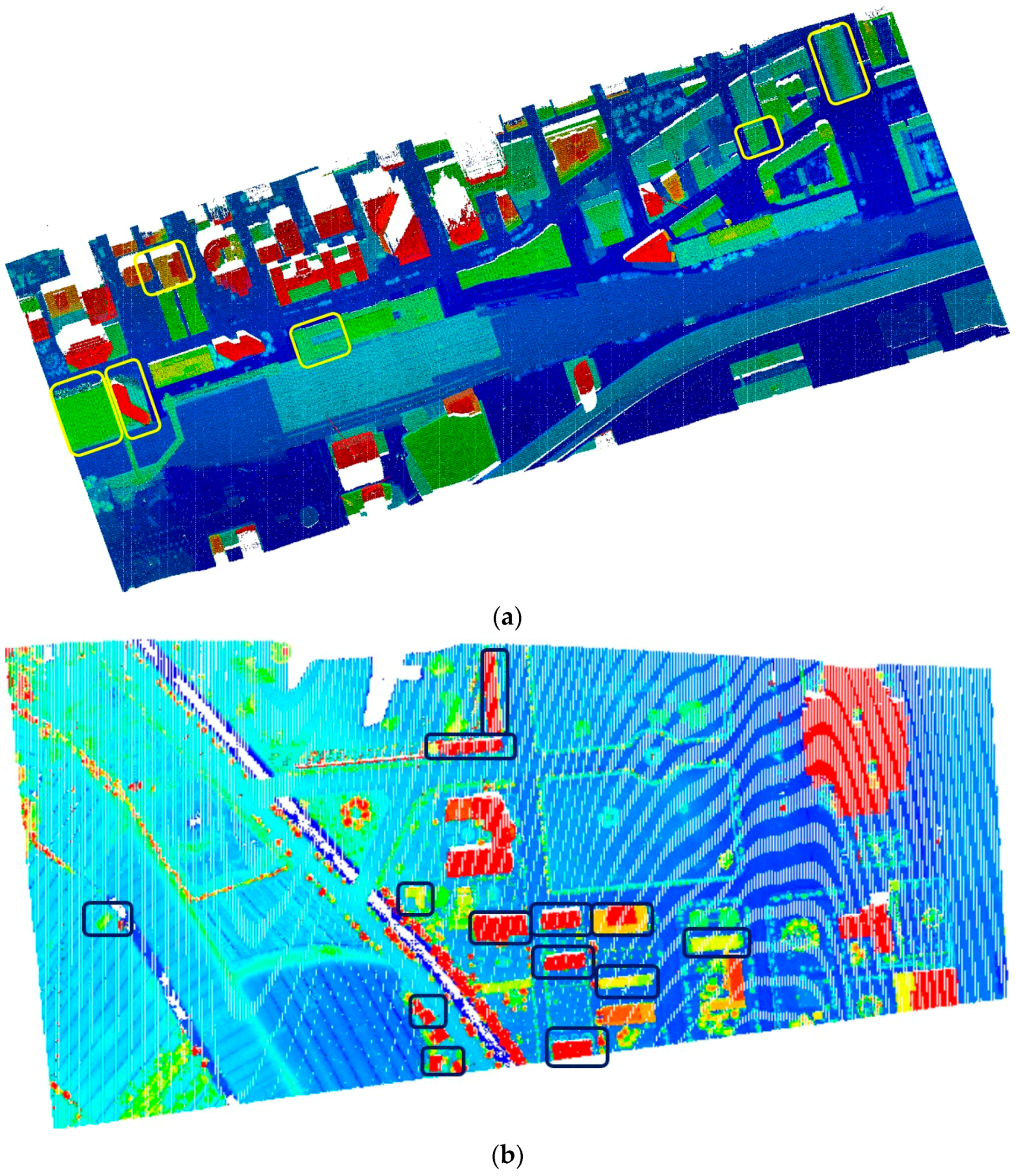
Two cases were included in this part. Each case contains two trajectories’ point cloud. The first case are located in Toronto and were captured in the year 2011. The two trajectories contained 2,727,981 points and 1,928,393 points. The typical objects in the case dataset were buildings, roads, grasses, and trees. The average point distance of the datasets was approximately 0.6 m. A part of the direct overlapping of these two datasets can be seen in Figure 4. There were obvious offsets and a slight rotation between the two datasets. The translation between the two datasets can be estimated by calculating the distances of a number of manually selected corresponding points. The result was approximately 4.1 m on average.

The second case are located in Zhoushan, a city of Eastern China and were captured in the year 2008. Two trajectories contains 356,489 and 784,271 points. Typical objects in this case were buildings, roads, trees, and water. The point density was 2.4 points/m². The case area is near the airport of Zhoushan; therefore, buildings here were very simple. Flat roofs and gable roofs are two main roof types included in the dataset. The difference between two trajectories’ point is relative large. A preliminary evaluation of difference of two trajectories point cloud is about 25 m on average.

In this study, both two trajectories’ datasets of two area were used to compute the registration parameters. The selection of building roofs and the alignment parameters were listed in Section 3.2 and Section 3.3. A comparison between proposed method and the other methods, like ICP and LMS were also listed in Section 3.3. Then, some further analysis, including the accuracy evaluation and error sensitivity evaluation was furnished by the first dataset because of the complexity of this dataset. The results will be given in Section 3.4 and Section 3.5.

3.2. Selection of Building Roofs for Registration

First of all, buildings have to extracted from the point clouds. In this work, an OSM-aided approach [23] is applied for this task. Considering the fact that the translation of two datasets is normally not that much, the buildings in the point clouds corresponded with the same building footprint will be regarded as corresponding buildings. In the next step, building roofs are segmented using the method presented in the same paper [23]. Only those buildings are selected if their roofs contain none or one ridge. In other words, the corresponding buildings are selected for further process, only when their roofs are simply constructed. Then feature regression method were applied to the point cloud of the selected building roofs.

In total, six buildings roofs of the first case were selected for the registration because their roofs are simple structures. In Figure 4, the polygons denote the locations of the selected buildings and the color denotes the elevation of point cloud.

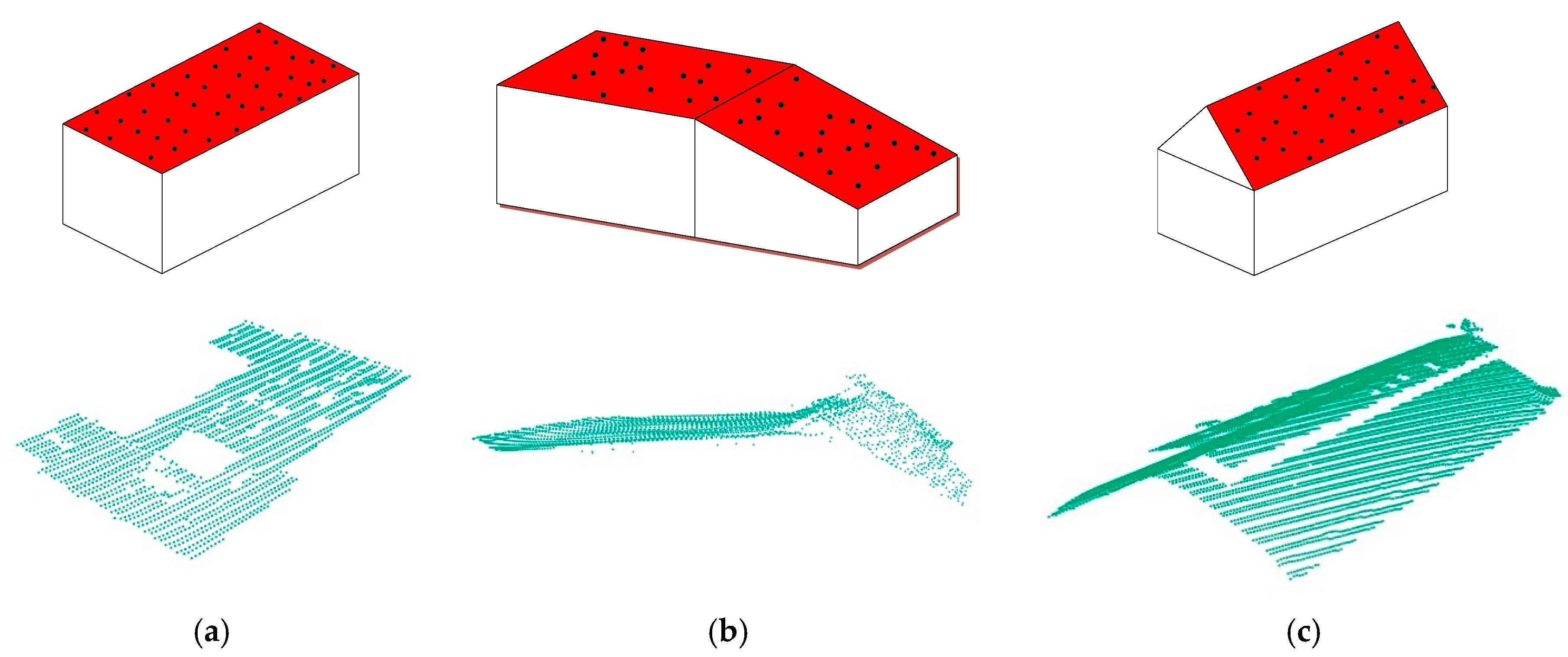
According to previous studies, there are over 33 types of roofs exists in the world, such as flat, gable, hip, L-joint, T-joint, etc. [24]. In this paper, three simple types of roofs were adopted: flat, slope, and gabled roof (see Figure 5). These three roof types are very common and typical in urban areas and is easy to fit the plane parameters from point cloud. Moreover, to avoid an ill-conditioned matrix in the observation system when using the least square method, different types of roofs with more points are recommended for use.

In the next step, the normal vectors of these roof facets were calculated and used to estimate the transformation between the two datasets. The results are shown in 3.3.

3.3. Estimation of Transformation Parameters

In this subsection, several buildings of each dataset were selected from the original point cloud and the normal vectors were computed. Then the transformation parameters were then calculated by normal vectors. As a comparison, two methods, ICP and LS, were selected to verify the validity of parameters. The source code of ICP were downloaded from https://github.com/charlienash/nricp. During the LS processing, nine homonymous points for each dataset were manually selected to compute the parameters.

■

Parameters comparison for the first case

Six buildings with 10 different roofs were selected for the first case area. The transformation parameters were computed and listed in

Table 1. Comparison of transformation parameters for the first case.

Parameters	Method	Value
$\left(\Delta x,\Delta y,\Delta \mathrm{z}\right)$	Proposed method	$\left(-0.840,-2.109,0.351\right)$
	ICP	$\left(-1.286,-2.391,0.358\right)$
	LS	$\left(-0.827,-1.941,0.370\right)$
R	Proposed method	$\left[\begin{array}{ccc}1.00231078858& 0.0151900835& 0.0002490458\\ 0.0042444902& 0.9990222473& 0.0006161759\\ -0.0001060228& 0.0000582398& 1.0000560232\end{array}\right]$
	ICP	$\left[\begin{array}{ccc}0.9999526948& -0.0097251967& -0.0001690211\\ 0.0097250337& 0.9999522693& -0.0009395809\\ 0.0001781506& 0.0009378928& 0.9999995443\end{array}\right]$
	LS	$\left[\begin{array}{ccc}0.9998695268& -0.0138030552& 0.0083907681\\ 0.0137186482& 0.9998555364& 0.0100351809\\ -0.0085280720& -0.0099187616& 0.9999144414\end{array}\right]$

.

■

Parameters comparison for the second case

Thirteen buildings with 15 different roofs were selected for the second case. Normal vector of planes were calculated and introduced into the proposed method; the transformation parameters, both proposed method, ICP method, and LS method were computed and listed as following. As the difference between two trajectories is obvious, a preprocessing to roughly co-register the two trajectories’ data is performed for ICP and LS methods. The results were listed in

Table 2. Comparison of transformation parameters for the second case.

Parameters	Method	Value
$\left(\Delta x,\Delta y,\Delta \mathrm{z}\right)$	Proposed method	$\left(-31.430,-7.947,-0.139\right)$
	ICP	$\left(-23.635,41.723,0.104\right)$
	LS	$\left(-24.209,-0.156,0.353\right)$
R	Proposed method	$\left[\begin{array}{ccc}0.9999034331& -0.0001935506& 0.0005516807\\ -0.0002691125& 0.9999946061& 0.0001537416\\ 0.0009099559& 0.0001823840& 0.9999401501\end{array}\right]$
	ICP	$\left[\begin{array}{ccc}1& -0.0000000017& -0\\ 0.0000000042& 1& -0\\ 0.0000000791& 0.0000000393& 1\end{array}\right]$
	LS	$\left[\begin{array}{ccc}0.99999688564& 0.0021268808& 0.0013057830\\ -0.0021220269& 0.9999908760& -0.0037074001\\ -0.0013136563& 0.0037046177& 0.9999922750\end{array}\right]$

.

Compared with the above parameters, the rotation matrix of proposed method is quite similar with the ICP and LS method. However the shift parameter is quite different because the difference between two trajectories is quite large.

3.4. Accuracy Evaluation

In order to evaluate the accuracy for proposed method, the first case was selected because the buildings in first case is relative more complex. Here, checkpoints as well as the two overlap buildings were selected to verify the difference after transformation. The horizontal distance of checkpoints were computed to evaluate the horizontal accuracy, while the overlap difference were computed to evaluate the vertical accuracy.

3.4.1. Accuracy Evaluation by Checkpoints

To evaluate the horizontal accuracy of registration, 40 checkpoint-pairs were selected, and the checkpoint distances were measured. The checkpoint-pairs were manually chosen in 2D point cloud view and most of them were building corners. The horizontal distance of each checkpoint pair was used as the index to evaluate the accuracy after the registration. Some statistical values, such as minimum, maximum, and average, were also computed. Table 1 shows that the horizontal distance ranged between 0.195–1.628 m, with an average distance of 0.964 m, which was approximately 1.6 times the average resolution of the raw point cloud (0.60 m). As a comparison, the same values from point cloud which were transferred by transmission parameters calculated by ICP method and LS method were also computed and shown in

Table 3. Accuracy of the checkpoints (m).

Index	Average	Minimum	Maximum
Proposed method	0.964	0.195	1.628
ICP method	2.190	0.046	4.690
LS method	1.668	0.300	2.504

. Results show that the average, minimum and maximum value between checkpoint-pair by proposed method is greater than ICP method and LS method.

3.4.2. Accuracy Evaluation by Overlap Zones

Different trajectories’ point clouds are usually captured from different points of view and overlap zones exist from adjacent trajectories’ point clouds. Here two overlapping buildings were selected to evaluate the residuals after registration. The purpose of overlap zone evaluation is to find the registration results in the overlap area by measuring the overlay difference, which also means the vertical distance. The first overlap area was a simple building’s roof with 5522 points in C1 data and 3689 in C2 data. The second area was a complex building with three main roofs and some skylights. One of the three roofs was sloped, and the other two roofs were horizontal. The number of points in the second area were 6635 in C1 and 4597 in C2. The isolated point clouds of both overlap areas were removed to reduce the effect of the noisy points.

In this part, three main steps were performed for each overlap zones. First, for each point of the transferred C1 dataset, a distance computation was performed to find the nearest point in the C2 dataset. The nearest distance was used to estimate the difference between the transferred C1 and the C2 datasets.

The graphical result for the first overlap area is shown in Figure 6. The maximum distance of the case area was approximately 0.310 m, and the average distance was 0.045 m.

The distribution of the difference levels was also analyzed in this paper. According to the minimum and maximum values of the differences, the residual data were sliced into seven classes. The number of points of each class was then counted; the obtained percentage and cumulative percentage are listed in

Table 4. Number of points in different layers of overlap zone-1.

Class (m)	# Points	Percentage (%)	Cumulative Percentage (%)
0.00–0.05	4002	72.47	72.47
0.05–0.10	812	14.70	87.17
0.10–0.15	427	7.73	94.90
0.25–0.20	229	4.14	99.04
0.20–0.25	43	0.77	99.81
0.25–0.30	8	0.14	99.95
0.30–0.35	1	0.01	99.96

. We found that most of the transferred C1 points matched the C2 dataset well, which also demonstrates that the computed transformation model parameters were able to match the different datasets of the point clouds.

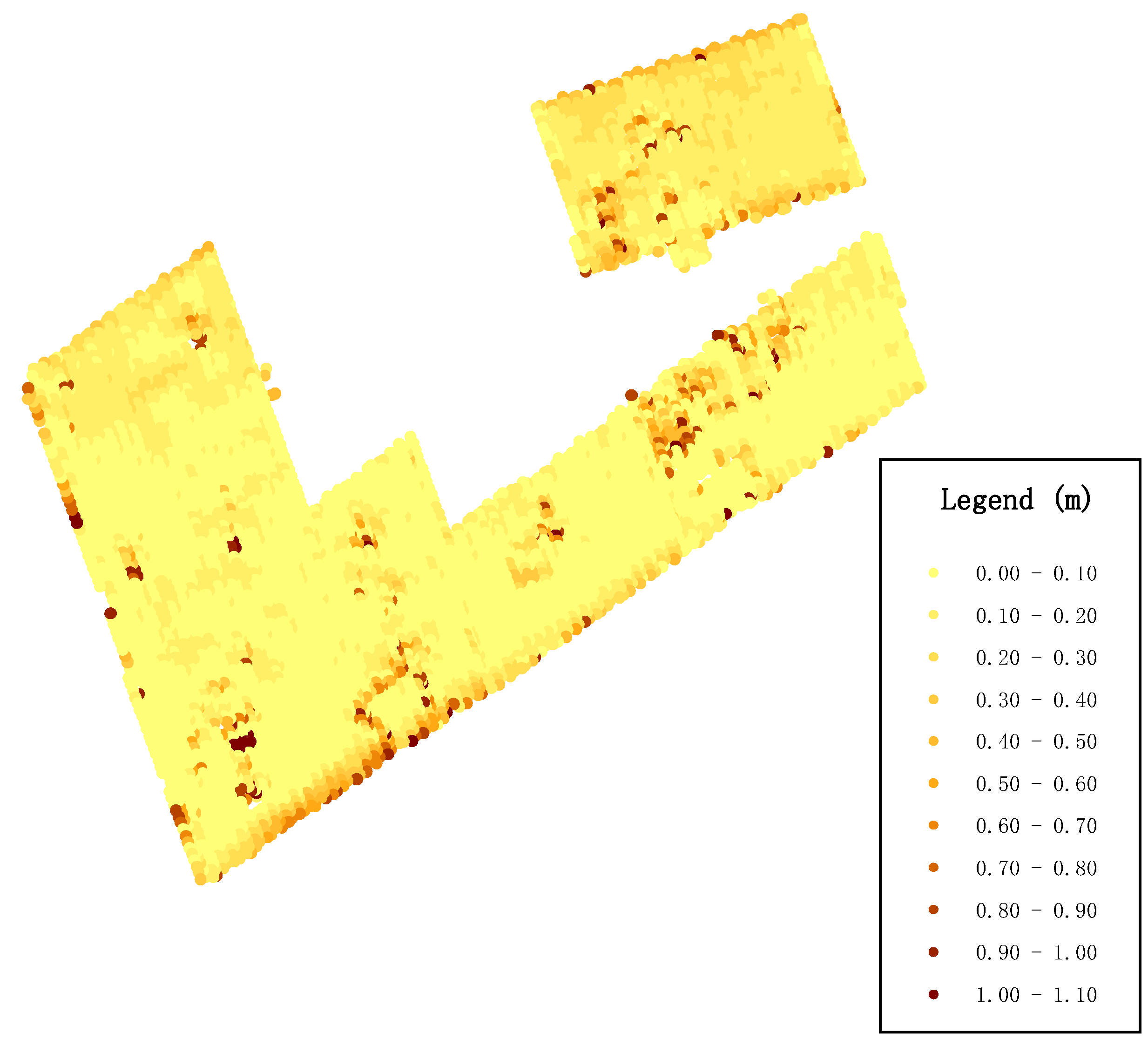
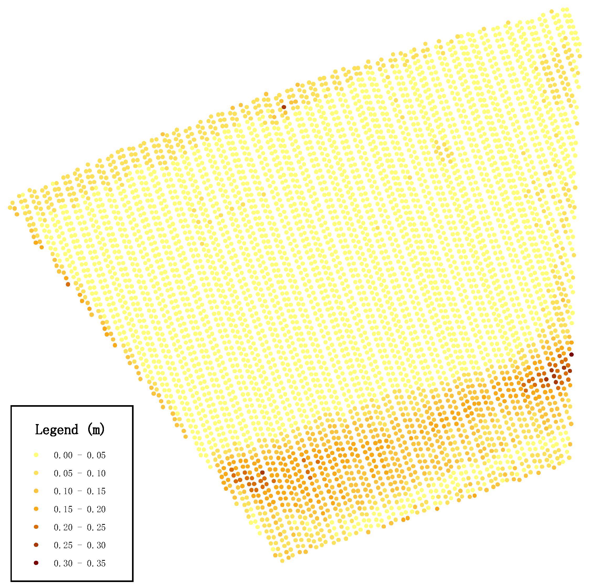
The graphical result for the second overlap area is shown in Figure 7. The maximum distance of the case area was approximately 1.100 m, and the average distance was 0.129 m.

Then, eleven levels were used to divide the points to analyze the distribution of different residuals. The number of points, percentage and cumulative percentage were then calculated; the results are listed in

Table 5. Number of points in different layers of overlap zone-2.

Class (m)	Points	Percentage (%)	Cumulative Percentage (%)
0.00–0.10	3763	56.71%	56.71%
0.10–0.20	1803	27.17%	83.89%
0.20–0.30	508	7.66%	91.54%
0.30–0.40	176	2.65%	94.20%
0.40–0.50	127	1.91%	96.11%
0.50–0.60	74	1.12%	97.23%
0.60–0.70	48	0.72%	97.95%
0.70–0.80	38	0.57%	98.52%
0.80–0.90	42	0.63%	99.16%
0.90–1.00	27	0.41%	99.56%
1.00–1.10	29	0.44%	100.00%

. According to the table, over 90% of the point-surface distances were lower than 0.30 m, demonstrating good quality in the results.

3.5. Error Sensitivity Evaluation of Proposed Method

Section 3.3 demonstrate that the proposed method can be used to compute the transformation parameters. However, the roof features regression processing will always be affected by the sensor error and noise. Therefore, this subsection is designed to evaluate the effect of random errors and demonstrate the stability for the proposed method.

In order to compare the transformation parameters calculated by proposed method with real parameters. We temporarily computed the C3 data which was transformed by C1 with the parameter, ${\left(\Delta x,\Delta y,\Delta \mathrm{z}\right)}_{true}$ and $R_{true}$:

$${\left(\Delta x,\Delta y,\Delta \mathrm{z}\right)}_{true}=3748.245,1569.256,12.235$$

The $\left(\mathsf{\alpha },\mathsf{\beta },\mathsf{\gamma }\right)$ were set with the value of 1.2°, 2.2°, 3.2° degrees separately. Then, according to the calculation equation, the true value of the rotation matrix is:

$$R_{true}=\left[\begin{array}{ccc}0.9981769128& 0.0209269835& 0.0566119425\\ -0.0230521610& 0.9990437615& 0.0371505100\\ -0.0557803598& -0.0383878090& 0.9977048298\end{array}\right]$$

The ${\left(\Delta x,\Delta y,\Delta \mathrm{z}\right)}_{true}$ and $R_{true}$ will be treated as the true transformation parameters between C1 and C3.

The transformation parameters were, firstly, computed according to the proposed method, and then the difference between computed parameters and true value is calculated (See first line of

Table 6. Rotation and shift parameters difference after random error added.

Scope of Random Error (m)	Rotation Matrix Difference	3D Shift Parameter Difference (m)
[−0.000, 0.000]	$\left[\begin{array}{ccc}6E-13& 2E-12& 1E-12\\ -3E-12& -7E-13& -4E-12\\ -2E-13& 3E-13& 2E-13\end{array}\right]$	$\left(\begin{array}{c}0.000\\ 0.000\\ 0.000\end{array}\right)$
[−0.001, 0.001]	$\left[\begin{array}{ccc}3E-6& -3E-6& 1E-6\\ -1E-5& -2E-6& -4E-6\\ -1E-6& 5E-7& 7E-7\end{array}\right]$	$\left(\begin{array}{c}0.000\\ 0.000\\ 0.000\end{array}\right)$
[−0.025, 0.025]	$\left[\begin{array}{ccc}-1E-4& 3E-4& 1E-4\\ 9E-4& 4E-4& 1E-4\\ 8E-6& -1E-4& -4E-5\end{array}\right]$	$\left(\begin{array}{c}-0.044\\ -0.011\\ -0.006\end{array}\right)$
[−0.050, 0.050]	$\left[\begin{array}{ccc}2E-4& 5E-4& -7E-4\\ 6E-4& -7E-4& -6E-4\\ 8E-6& -4E-4& -1E-5\end{array}\right]$	$\left(\begin{array}{c}-0.015\\ -0.005\\ -0.006\end{array}\right)$
[−0.100, 0.100]	$\left[\begin{array}{ccc}1E-4& -2E-3& 5E-4\\ 3E-3& 1E-3& 8E-4\\ -4E-5& 4E-4& 1E-5\end{array}\right]$	$\left(\begin{array}{c}0.190\\ 0.035\\ 0.049\end{array}\right)$

). Then, four levels of random errors were added to each point of C3 to testify the effect of random errors for proposed method. Then, transformation parameters, as well as the difference between computed parameters and real values were calculated again (See line 2–4 of Table 6).

The last two columns of Table 6 are calculated by the true value minus the computed transformation parameters in this experiment. We can find that once random errors were added to the original point cloud, the sensitivity of the rotation matrix is obvious because the components’ differences of rotation matrix decreased from about 1 × 10⁻¹² to 1 × 10⁻⁶ rapidly. However, as the random error increased from 0.001 m to 0.100 m, the components difference decreased slowly (from about 1 × 10⁻⁶ to 1 × 10⁻⁴). From the last column of above table, the shift parameter difference is relevant with the scope of the random errors. Once the scope of random error is relatively small, the difference of the 3D shift parameter is low.

3.6. Visualization of the Matched Point Cloud

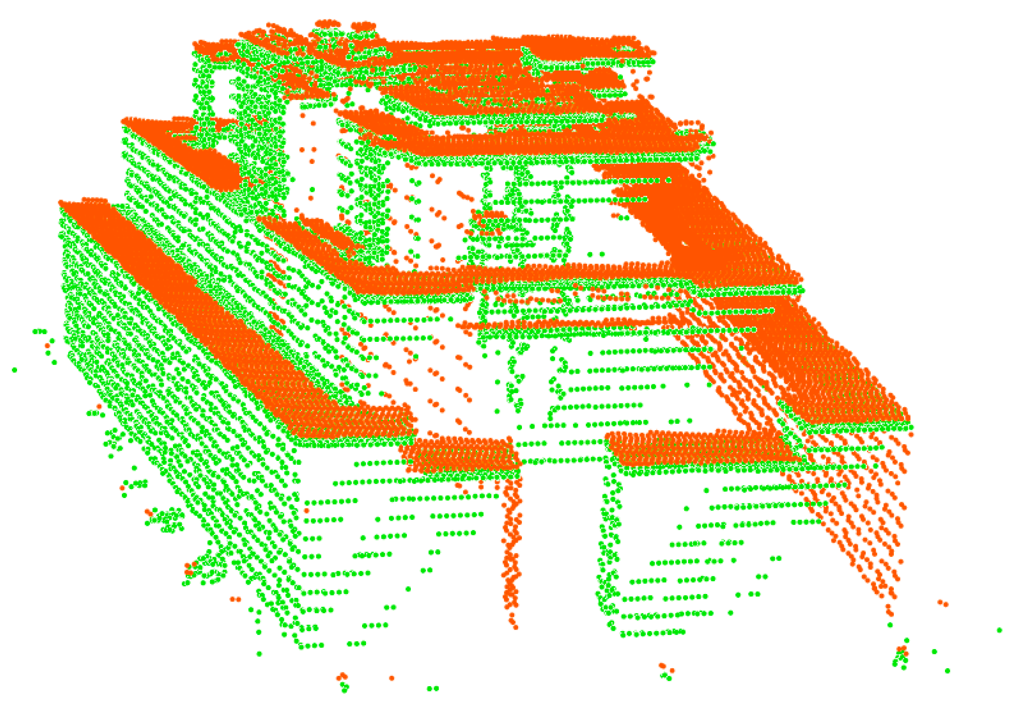
Applying the transformation parameters distributed in Section 3.2, the point cloud of trajectory 1 was transferred. Figure 8 shows the results of a complex building in the case area, which demonstrates that the proposed method achieved good results. The two colors of the figure denote the trajectory number: the orange color denotes the first trajectory, and the green color denotes the second trajectory.

4. Discussion

Although the mathematical calculations of the proposed method are simple, two strict requirements are required when applying this approach. The first requirement is that the direction of normal vectors of plane-pairs should be the same in both datasets. The normal plane regression method will provide a normal vector $\left(\begin{array}{ccc}A& B& C\end{array}\right)$ and the constant value (D) as the plane parameters. These parameters will satisfy the plane equation AX + BY + CZ = D; however, the negative form of the normal vector $\left(\begin{array}{ccc}-A& -B& -C\end{array}\right)$ and the negative constant value ($-D$) also satisfy the plane equation. We must choose the proper form of the plane parameters and establish suitable plane-pairs. In this paper, an additional operation was applied to the regressed plane parameters. An angle between the normal vector and the Z axis was used to evaluate the status of normal vector. If the angle was over 90 degrees, then we used the negative form of the normal vector in the relevant equations.

Another requirement to use the proposed method is the selection of a variety of normal vectors, i.e., the building planes used to calculate the model parameters should point in different directions. More than three different directions are recommended. In this paper, we selected three types of building planes, and among six normal vectors, three different directions were used. This will prevent the matrix $({V_2}^{\prime }{V}_2)$ from becoming an ill-conditioned matrix and lead to a successful solution. Meanwhile, as a rotation matrix, an additional requirement, det(R) = 1, should be satisfied during the calculation.

For most registration research, control points are the common features used to compute the registration parameters. In this paper, plane roof features were used instead of control points, and good results were achieved. However, the detailed principle of adjustment by roof features still requires a mathematical discussion. Moreover, as the real transformation parameters are unknown, the estimated parameters by control points or control planes are approaching the real values. Moreover, the distribution of the selected roof features is important for the calculation of the model parameters. The selection of more features or the altering of other features will lead to different results. Therefore, we suggest that the user selects roof features by equal distribution.

5. Conclusions

This paper proposed a method using the linear plane of buildings as the sources of feature-based data registration. A three-step calculation method of the model parameters was introduced. The first step of the method is to select the simple-structured buildings with the assistance of OpenStreetMap (OSM). Then, the normal vectors of the selected building roofs are computed using a fitting program and then are introduced into an observation system to obtain the proper translation and rotation parameters. Last, the rotation and shift parameters of the 3D rigid body model are applied to the point cloud to be matched. Two trajectories’ point clouds were used to verify the validity and accuracy of proposed method. According to the experimental results, the proposed method achieved good results and can be used to co-reference the adjacent point cloud.

The novelty of this paper is that the linear features of the corresponding roof facets were used for the estimation of the registration parameters instead of the corresponding points. This process avoids the large ambiguity when selecting corresponding points manually and reduces the cost when using artificial objects as the corresponding points.