Article

Multi-Decadal Monitoring of Lake Level Changes in the Qinghai-Tibet Plateau by the TOPEX/Poseidon-Family Altimeters: Climate Implication

1
Department of Civil Engineering, National Chiao Tung University, 1001 Ta Hsueh Rd., Hsinchu 300, Taiwan
2
School of Geodesy and Geomatics, Wuhan University, Wuhan 430079, China
*
Author to whom correspondence should be addressed.
Remote Sens. 2016, 8(6), 446; https://doi.org/10.3390/rs8060446
Submission received: 9 March 2016 / Revised: 10 May 2016 / Accepted: 18 May 2016 / Published: 25 May 2016
(This article belongs to the Special Issue Remote Sensing in Tibet and Siberia)

Abstract

:
Lake levels in the Qinghai-Tibet Plateau (QTP) provide valuable records for climate change studies. We use two decades of measurements (January 1993–December 2014) from the TOPEX/Poseidon (T/P)-family satellite altimeters (T/P, Jason-1 and -2) to detect lake level variations at 23 lakes along their repeat ground tracks every 10 days. We employ an optimal processing technique to obtain quality measurements, including outlier detection, averaging and filtering. The lake level accuracies are improved by subwaveform retracking. Jason-1 delivers few measurements after waveform retracking and a cluster classification at most lakes. From January 1993 to December 2014, most lake levels in eastern Tibet rose, while those in western Tibet declined. In Qinghai, lake levels dropped before 2005 and then rose afterwards, coinciding with the measure in 2005 that protects the Qinghai ecosystem (e.g., grassland conservation). The overall pattern of lake level change in the QTP is largely affected by monsoons and lake locations. Most lake levels show clear annual and inter-annual oscillations. Certain lakes show alternating level highs and lows in the same seasons and varying amplitudes of annual oscillations due to lake level changes. We detect a sudden rise of lake level by 7 m caused by floods, varying lake level trends associated with the 1997‒98 El Niño and other factors, and persistently rising and declining lake levels associated with the long-term precipitation trends in the QTP. The T/P-family satellites will continue to monitor lake levels here as long as the sea level monitoring program lasts, collecting a long-term climate record at highlands echoing sea level change.

Graphical Abstract

1. Introduction

The Qinghai-Tibet Plateau (QTP) is home to a large number of inland lakes. Due to rare human interference and high altitudes (mean altitude: 4500 m), variations of lake levels in the QTP are largely attributed to natural causes. Two dominant factors contributing to the variations are precipitation and glacier state [1]. Compared to lakes at low altitudes, high-altitude lakes in the QTP could receive water from runoffs of melting glaciers, whose rates are mostly affected by temperature variations. As confirmed by satellite- and ground-based observations, recent global warming has accelerated glacier melting rates in the QTP, thereby altering the rates of lake level changes here [1,2]. This implies that lake level change in the QTP is closely linked to global climate change [3,4]. Globally, the increase of lake temperature tends to be greater than the increase of sea-water temperature [5], adding another uncertainty to the state of QTP lakes.
Due to the inaccessibility and the vast area of the QTP, most lakes here lack in situ elevation measurements, resulting in poor information about lake level change. As such, variations of lake levels in the QTP are largely based on observations from satellite borne and airborne sensors. For example, Li and Wang [2] used satellite optical images to detect areal changes of Bam Co, Pung Co, Dung Co and Nuripung Co in Nagqu, and showed how such changes are connected to climate change. “Co” means lake in Tibetan. They found that the areas of the four lakes have increased steadily since 2005 due to a wetter QTP climate. They attributed climate change to increases in atmospheric temperature, precipitation, evaporation and melting glaciers and permafrost. Shao et al. [6] found similar results for these four lakes. Huang et al. [4] used SRTM elevations and optical images to investigate the link between the area changes of 12 lakes and climate change in the past four decades in Nagqu, concluding that most of the 12 lakes have expanded lake areas. Yao et al. [7] used Landsat TM/ETM+ images to study lake areas in the Hoh Xil region and found that the lake areas shrank before 2005, and then expanded afterwards. Due to limited resolutions of optical images and data discontinuity, only rough trends in lake area changes can be obtained in these studies.
A major sensor for detecting lake level change is satellite radar altimetry. Originally designed for use in oceanography, ice sheet dynamics and land surface change, radar altimetry is also used to monitor lake level changes. For example, Morris and Gill [8] used TOPEX/Poseidon (T/P) altimeter to detect level changes in the Great Lakes of North America, achieving a 2.9 cm RMS difference with in situ lake gauge measurements. Alsdorf et al. [9] used T/P altimeter data and JERS-1 SAR images to detect lake changes in Amazon, identifying a key relation between lake level change and climate change. Hwang et al. [10] used T/P altimetry to obtain 10 years of lake level time series in 6 inland lakes of China, and identified the dominating oscillations and decadal trends in these lakes. From the T/P altimetry, Hwang et al. [10] also found reversed lake level trends of Ngangzi Co caused by the 1997‒98 El Niño.
Another type of satellite altimetry for lake level observations includes laser (e.g., ICESat) and SAR Interferometry (SARIn, e.g., Cryosat-2). The only existing satellite-borne mission of laser altimetry is ICESat. Zhang et al. [1] used ICESat to detect level changes of 111 lakes over 2002–2009 in the QTP, and found that levels at 74 lakes were rising. Song et al. [11] used ICESat to detect abrupt and seasonal lake level changes in the QTP and classified the changes in various clusters that were explained by climate patterns. Kleinherenbrink et al. [12] used Cryosat-2 SARIn mode data to monitor lakes level over 2012–2014 in Tibet and Tian Shan, and divided lakes in four classes depending on the number of Cryosat-2 passes that were actually used. Unlike the repeat orbit configurations of radar altimeter missions such as the T/P-family satellites, ICESat and Cryosat-2 collected height observations in cycles and subcycles over lakes, resulting in lake heights at non-uniform time intervals.
The objective of this paper is to determine optimal lake levels and their changes from radar altimeter missions T/P, Jason-1 (J1), and Jason-2 (J2) in the QTP. T/P, J1 and J2 are a family of radar altimeters, spanning data from October 1992 to present. They repeat the same ground tracks every 10 days on 254 passes. Despite the large cross-track spacing of 157 km (counting both ascending and descending tracks), along-track observations on a pass can be collected at an interval of 660 m or 330 m using the 10- or 20-Hertz (HZ) radar measurements. For a lake visited by the T/P-family satellites and with a favorable radar observing condition (see Section 3.1), multiple decades of lake level changes can be derived. Compared to the laser altimeter satellite ICESat, the T/P-family satellites can measure lake levels at uniform time intervals and form time series for detecting variabilities at different time scales. In this paper, we will identify 23 lakes in the QTP that can be monitored from 1993 to the times of future TP-family altimeters such as Jason-3 (J3) and beyond. This paper will demonstrate that, detecting long-term lake level changes is another valuable application of the T/P-family satellites, in addition to sea level change, ocean circulation and ocean tide.

2. Radar Altimeter Data of TOPEX/Poseidon-Family Satellites for Lake Level Change

The T/P-family satellites, the altimeter data and the auxiliary data for this study are summarized below. First, Figure 1 shows the repeat ground tracks of T/P-family satellites around the QTP. Figure 1 also shows the identification numbers of 23 lakes that are of a sufficiently large (area > 36 km2) to yield reliable multi-decadal lake levels (January 1993 to present, even with follow-on missions for another few decades). Table 1 gives selected information about the 23 lakes. Both geophysical data records (GDRs) and sensor data record (SDRs) are needed in this study (For more detail, see [13]). GDRs contain orbit heights and range measurements, and geophysical corrections. SDRs contain radar waveforms for range refinements (see Section 3.1). Unlike T/P, missions J1 and J2 merge GDRs and SDRs into one record, called Sensor Geophysical Data record (SGDR), over January 2002–December 2008 (J1) and July 2008–December 2014 (J2). All altimeter data, including GDRs, SDRs and SGDRs (For more detail, see [14,15]), are downloaded from the French space agency AVISO [16].
Launched on 10 August 1992, T/P is the first of the family satellites, ending in January 2006. Considering the data quality, we used T/P records only from 1 January 1993 to 11 August 2002 (cycles 011-364). J1 is a follow-on mission of T/P over December 2001–July 2013. Before February 2009, J1’s orbit parameters were exactly the same as T/P’s. From 2009 onwards, J1 orbit was maneuvered into a geodetic orbit focusing on collecting data for marine gravity and bathymetry. J1 lasted through 2013 and its data have greatly advanced marine geophysics. J1 carried a Center National d'Etudes Spatiales (CNES)-made dual frequency altimeter (Poseidon-2), a tri-band radiometer and a combined DORIS-GPS tracking system. On land, the wet tropospheric delays of J1 altimeter ranges were corrected using the ECMWF (European Center for Medium-Range Weather Forecasts) model. However, most J1 observations on land are deteriorated by bad waveforms [17]. Our data processing of J1 (Section 3) shows that the qualities of J1 waveforms vary with location and time. Sometimes, J1’s bad waveforms can result in ranging errors of up to 100 m which cannot be mitigated by waveform retracking (see Section 3.1). By a careful data screening and cluster analysis, we still obtain some good lake level observations from J1 over certain lakes (see Section 3.2).
J2 is a joint mission of National Aeronautics and Space Administration (NASA), CNES and European Organization for the Exploitation of Meteorological Satellites (EUMETSAT) and National Oceanic and Atmospheric Administration (NOAA) and launched in June 2008. It continues the efforts of T/P and J1 and still functions today. J2 is commonly called OSTM/Jason-2 with OSTM standing for Ocean Surface Topography Mission. As the names implies, J2 is designed for ocean mapping and has exactly the same orbit parameters of its predecessors. J2 carries a Poseidon-3 altimeter for ranging, an Advanced Microwave Radiometer (AMR) for mapping the troposphere and a DORIS-GPS system for orbit determination.

3. Determining Reliable Lake Levels from Radar Measurements

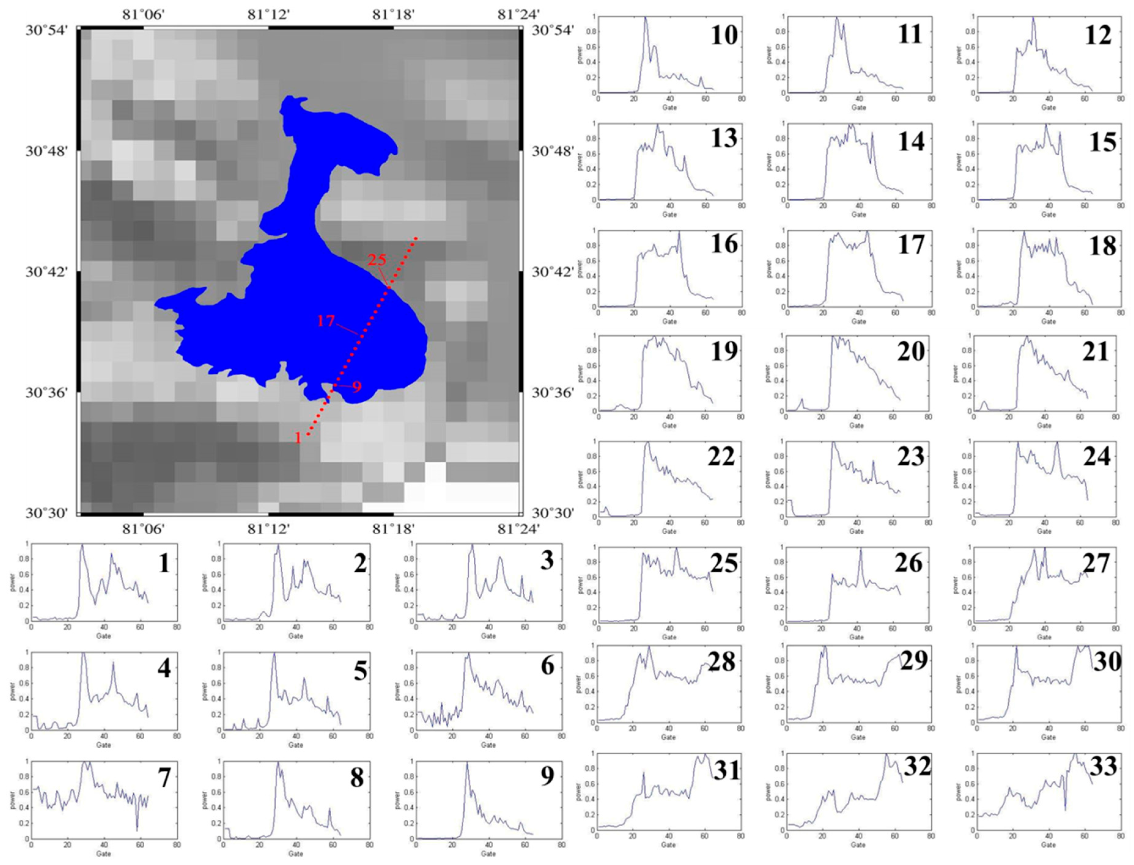
3.1. Improving Lake Level Measurements by Retracking Waveforms

Over a lake, a radar altimeter transmits radar pulses to measure the range (vertical distance) between the satellite and the lake surface. A lake level, LL, is the difference between the satellite’s ellipsoidal (geodetic) height and the range:
L L = h s a t R a l t C
where h s a t is satellite’s geodetic height, R a l t is the range measurement, and C is a term containing corrections and can be expressed as
C = C C O G + C w e t + C d r y + C i o n o + C s o l i d + C p o l e + C r e t r a c k
The first six terms on the right-hand side in Equation (2) are corrections for center of gravity, wet tropospheric delay, dry tropospheric delay, ionosphere, solid earth tide and pole tide. Unlike altimeter-height measurements over oceans, there is no need of ocean tide correction, inverse barometer correction and sea state bias correction over lakes. The last term in Equation (2) is the range correction from waveform retracking (see below for the detail). Except C r e t r a c k , all the needed corrections are provided in the GDRs of the satellites (Section 2). Because the radiometers of the three satellites did not yield measurements on land [10], the tropospheric delay corrections on land for three satellites are based on the ECMWF modeled values.
As shown in Shum et al. [24] and Lee [25], the correction for tracking gate, C r e t r a c k , is critical to precision land surface heights (including lake levels) from radar altimetry. C r e t r a c k can be obtained by waveform retracking. Several algorithms for waveform retracking are available in the altimetry literature, such as Beta-5 [26], off-center of gravity (OCOG) [27], the sea-ice algorithm [28], the threshold algorithm [29], the improved threshold algorithm [30], and the subwaveform algorithm [31]. Based on the previous experiments [31,32,33], in this paper we adopt the algorithm of subwaveform retracking [31] for all three satellites. For brevity, the algorithm is called subwaveform retracking. T/P’s SDRs contain waveforms at the 10-Hz frequency with each waveform having return powers at 128 gates. This format is different from those of J1 and J2 that have 104 gates. To facilitate our computations, for each T/P waveform we re-sampled the powers at 128 gates to powers at 64 gates, following the strategy of Lee [25]: at the original T/P gates 1–16 or 49–64, we averaged the powers at two consecutive gates to determine the power at a new gate; at the original T/P gates 65–128, we averaged the powers at 4 consecutive gates to determine the power at a new gate. The powers at the original T/P gates 17–48 were exactly the same as those at the resampled gates. For all satellites, the default tracking gate will be modified based on waveform retracking. At a mean altitude of 4500 m, the states of lakes can be liquid, solid or at a mixed state depending on the surface temperature. Therefore, lake level changes on a high-altitude plateau are more complicated than lakes at lower altitudes. If a lake surface is covered by ice, the waveform is likely to be specular. In the interior of a large, deep lake, waveforms are likely to follow the Brown model [34].
For subwaveform retracking, a reference subwaveform with 22 gates is selected based on the Brown model [34]. As an example, here we use T/P waveforms to illustrate how the subwaveform retracking works. Beginning from a subset of waveform at gates 1–22 to the last subset at gates 43–64, each of the subsets is matched with the following standard subset of waveform (based on Brown model)
P ( t ) = A 2 [ e r f ( t τ 2 σ ) + 1 ] { 1 exp ( ( t τ ) / α ) t < τ t τ
where erf is the error function, P ( t ) is the power at time (gate) t, A is amplitude of the power, τ is the time corresponding to the center of the leading edge, α is an exponential decay parameter and σ is the slope of the ascending part of the waveform. The correlation coefficients between the subsets and the standard subset are determined. The subset with the largest correlation coefficient is then used to determine the new tracking gate by the threshold method [29] to refine the range. Further details of this method can be found in Yang et al. [31]. Because most of the waveforms over lakes in the QTP resemble waveforms in the open oceans, the best threshold value is 20%, which is typically used for threshold waveform retracking for waveforms in the open oceans [30,33]. The retracking re-defines the gate of the leading edge to obtain the following correction
C r e t r a c k = ( G R G T ) × 0.46875
where G T and G R are the gate numbers at the midpoints of leading edges from the default (onboard) setup and from the waveform retracking. The waveforms can also be used to determine surface types (land or lake).
Most waveforms of J1 over land, including lakes, are corrupted to the extent that only few range measurements can be derived from the waveforms. To improve J1’s data coverage over lakes, we applied the cluster analysis method and algorithm of Dabo-Niang et al. [35] to identify waveforms that are similar to the Brown (deep-lake) waveforms and specular waveforms. These waveforms were then retracked to determine range corrections.
Figure 2 shows T/P waveforms around La’nga Co at 33 spots, stretching a latitudinal range of 0.18°. The waveforms near the lake interior follow the Brown waveform shape (model) resembling those over oceans. The waveforms at spots 1–8 and spots 27–33 are irregular due to the land’s rugged surface and its large slope (>2°). The waveforms at spots 10–24 are on the lake surface and similar to waveforms in the deep oceans. The extreme case of a deep-lake waveform is the specular waveform. It is a special case of the ocean, Brown waveform with a sharp leading edge and a sharp trailing edge. Using the subwaveform retracking, we can also determine precise ranges from specular waveforms.

3.2. Constructing Lake Level Time Series at 23 Lakes

Here we list our steps to construct a time series of lake level change.
I. 
Select the best data session over a lake
Typically, only one pass is available over a lake. For cases with more than two passes, we select data from the pass that travels through the part of the lake with the best possibility to yield reliable heights. The best data session should be as close as possible to the central part of the lake to avoid land interference. This is to obtain range measurements with the best waveforms, as close as possible to oceanic waveforms. For example, T/P pass 181 travels through La’nga Co, the longitudes range from 81.26° to 81.28° and latitude 30.63°–30.66°. The best data session is around spot 17 (Figure 2).
II. 
Average heights from measurements in a cycle to form a representative height
Height measurements from a given cycle are first used to determine a mean height. Differences between heights at individual spots and the mean height, as well as the standard deviation are computed. Any height yielding a difference larger than 3 times of the standard deviation is removed. A new mean height is determined from the outlier-free heights. This data selection and averaging are iterated until no outlier is found, yielding a final, representative height for the lake from the given repeat cycle.
III. 
Form time series of lake level changes
For each lake, a mean height is computed using representative heights from all cycles. The differences between the representative heights from individual cycles (Step II) and the mean height are the lake level changes shown in Section 4.

4. Result

4.1. Trends of Lake Level Change: An Overview

For each of the 23 lakes, the altimeter-derived lake levels are modeled as:
H ( t ) + v = a + b t + c cos ( 2 π ω t ) + d sin ( 2 π ω t ) + e cos ( 4 π ω t ) + f sin ( 4 π ω t )
where H ( t ) is lake level change (Step III, Section 3.2), t is the time relative to the mean time, v is the residual, a is a constant, b is the trend, c 2 + d 2 and e 2 + f 2 are the amplitudes of the annual and semi-annual oscillations and ω is the annual frequency (one cycle per year). For each of the 23 lakes, the six parameters were determined by the least-squares method requiring that the sum of the squared residuals ( v ) be a minimum. An equal weight is given to all observations because of lack of a reliable method for estimating individual weights. The single largest factor affecting the rate of level change at a lake is outliers, which by all means must be removed; see the method in Section 3.2.
Figure 3a shows the trends of lake level change at the 23 lakes and the distributions of the westerlies, Indian monsoons and East Asian monsoons. The westerlies carry moistures from Europe and supply water to lakes largely in western Tibet. Recent intensification of the westerlies has caused mass gains in the Karakoram glaciers [36]. The Indian monsoons are the main contributors to rains in eastern Tibet and Qinghai. The extent of the Indian monsoons rains is governed by terrains and the traveling distance of the Indian monsoons. The lakes marked in red are lakes with rising trends and in blue are those with dropping trends over January 1993–December 2014. Among the 23 lakes, 12 lakes show a rising trend and 11 lakes show a decreasing trend. In terms of data quality, 8 lakes contain height observations from T/P, J1 and J2 (Eling, Kusai, Zhapu, Ngangzi, La’nga, Jiuru, Laorite, and Chibuzhang), representing the lakes with the most comprehensive observations with unambiguous long term changes. Eleven lakes contain both T/P and J2 observations. The remaining four lakes (Margog, Qingwa, Zhaxi, and Zhari Nam) contain observations from T/P or J2 only. Because J1 fails to deliver height observations in most of the lakes, in Table 2 we show rates from T/P only and J2 only.
There are only few climate stations in the QTP that provide long-term records of temperature, precipitation and evaporation. Huang et al. [4] showed that several QTP climate stations experienced rising temperatures and decreased evaporations during 1966–2010. The GPCP result in Figure 3b gives a larger picture of trends of precipitation, but the resolution is low at 2.5° × 2.5°. Figure 3b shows no clear boundary of positive and negative trends of precipitation. However, Figure 3b does show that regions in the Himalayas receive less rains and the QTP receives more rains over January 1993–December 2014. Such a pattern of rain in Figure 3b is in general consistent with the pattern of lake level change in Figure 3a. Although precipitation plays an important role in modulating the lake level, the exact causes of changes in the levels of the 23 lakes are complicated and not well understood.

4.2. Assessment of Lake Level Changes

Due to lack of in situ lake gauge records available to the authors, it is challenging to assess the uncertainties of lake level changes from T/P family satellites in the QTP. Here we made two indirect assessments by comparing the lake level changes derived from T/P family satellites (with the method given in Section 3) with in situ gauge records and Envisat results. The first assessment was made at Bosten Lake, where in situ gauge measurements from 1993 to 2001 (roughly the same period as T/P) are available to the authors [37]. Figure 4a compares the lake level changes from T/P with the in situ gauge data at Bosten Lake, which agree well with each other. This Bosten Lake records were also used in Hwang et al. [10], who also reported a similar assessment result like that given in Figure 4a. Lake level changes from Envisat at Bosten Lake are also shown in Figure 4a and are consistent with those from J1 and J2, despite a small inter-altimeter bias between Envisat and T/P-family (more details are given in Section 5.2). The Envisat data were obtained from the European Space Agency (ESA) and processed in the same manner as shown in Section 3. The steady decrease of Bosten lake level since 2003 detected by J1 and Envisat is consistent with the result of Wang et al. [38]. The other assessment is at Eling Lake. No gauge records at Eling Lake are available here, however, we obtained decadal precipitation records from a nearby weather station, provided by National Oceanic and Atmospheric Administration [39]. Figure 4b,c show the annual in situ precipitation records, as well as annual modeled precipitation, monthly lake level changes from T/P family and Envisat at Eling Lake. The modeled precipitation was derived from GPCP through a simple linear interpolation, and it agrees very well with the in situ precipitation records (Figure 4b). This also suggests that GPCP could provide useful estimates of rains in regions without observations in the QTP. Moreover, both in situ and modeled precipitations, around Eling Lake exhibit an increasing trend from 1993 to 2012. Both the J1 and Envisat lake level changes show a reversal of trend around 2004 (Figure 4c). However, the precipitation increased steadily since 2001 without a trend reversal in 2004. The cause for this trend reverse of lake level in 2004 is discussed in Section 4.3. These two assessments show that lake level changes from T/P family satellites are consistent with in situ measurements and results from Envisat. Hence, our processing approach for T/P family satellites is adequate at the 23 lakes.

4.3. Analyses of Lake Level Changes at Selected Lakes

In Section 4.1, we show a general pattern of lake level trends in the QTP. Here we provide more detailed analyses on lake level time series at selected lakes. According to different features of the lake level trends, we divided the selected lakes into three categories: (I) Lakes with varying lake level trends, (II) Lakes with continuous dropping trends, (III) Lakes with continuous rising trends. Analysis of each category will be presented in the following text.
(I) 
Lakes with varying lake level trends
Lake under ecological protection—Eling Lake (No. 1)
Here we focus on a lake in Qinghai: Eling Lake. Eling Lake is one of the sources to the Yellow River in China [40]. It receives inflow from a river to the west and flows northeastwards to the Yellow River. Figure 4c shows the lake level time series over January 1993–December 2014. There are no records of T/P from 1994 to 1995. Between January 1993 and January 2002, Eling’s lake level rose at a rate of 0.09 m/year. From January 2002 to June 2004, the lake level dropped rapidly at a rate of −0.84 m/year. In the summer of 2004, the lake level of Eling was too low to supply water to the Yellow River. From June 2004 to December 2008, Eling’s lake level rose at a rate of 0.74 m/year. From 2008 to 2014, Eling’s lake level dropped slightly. The major factors affecting such rapid changes in lake level trend are drought and overgrazing of grassland [4,6,7]. Since June 2004, the local government imposed a measure to protect the grassland in this region [41]. This measure, combined with increasing precipitations, is thought to raise Eling’s lake level.
Lake at risk of outburst flood—Kusai Lake (No. 2)
Kusai Lake is a glacial lake receiving water from melted glaciers of mountain and other glacial lakes. Here we report a surge of lake level of Kusai in 2011 detected by J2; see Figure 5. From 11 September to 21 September 2011, the Kusai lake level rose by 7 m and this dramatic rise is consistent with the in situ lake level observation that is reported on the web page of Administrative Bureau of Hoh Xil National Nature Reserve [42]. The sudden lake level rise can be caused by the flood from the Zhuonai Lake flowing into Kusai Lake [43]. As reported in Yao et al. [43], the heavy precipitation on 17 and 21 August led to an extra water outflow of Zhuonai Lake to Kusai Lake on 22 August 2011. Subsequent precipitations during 31 August to 9 September, and on 16 and 17 September caused a serious flood around Zhuonai Lake from 14 to 21 September, which increased the area of Kusai Lake from 290.23 km2 to 350.87 km2. This corresponds to a 21% increase in Kusai’s lake area, thanks to the flood-induced extra outflow of Zhuonai Lake.
This example raises the potential of an operational use of radar altimetry: over a sufficiently large glacial lake whose downstream areas are populated, an altimeter can deliver near-real time lake level heights to assess the risk of a glacial lake outburst flood (GLOF) and provide warnings. GLOF over a lake can be caused by heavy rain, avalanche, earthquake and temperature rise that leads to the failure of the dam holding a glacial lake. GLOF events in Tibet have been detected by, e.g., Fujita et al. [44], Liu et al. [45]. The sudden 7-m rise like the one in September 2011 at Kusai can overload a fragile dam to cause its failure, leading to a GLOF that threatens lives in its downstream areas.
Lake level changes associated with the 1997–1998 El Niño—Ngangzi Co (No. 12), Dagze Co (No. 14) and Gyarab Co (No. 15)
A previous study by Hwang et al. [10] has identified the reversed lake level trends of Ngangzi Co in 1998 associated with the 1997–1998 El Niño. Figure 6 shows the Niño 3.4 index (from the official site [46]) over 1993–2014. The Niño 3.4 index is a global indicator for intensity of El Niño. Figure 6 shows the exceptionally large temperature anomaly associated with the 1997–1998 El Niño. Based on the analysis of satellite images, Huang et al. [4] reported that the lake area of Dagze shrank by 7.45 km2 from 1970 to 2000, and then expanded by 46.49 km2 over 2000–2010. With the extended lake level time series and the refined lake level in this paper, here we show reserved lake level changes at Ngangzi Co (Figure 7a), Dagze Co (Figure 7b) and Gyarab Co (Figure 7c). With J1 observations available, the Ngangzi lake level is the most evident in depicting such a trend reversal (from −0.48 to 0.40 m/year), with less pronounced reversals at Dagze Co and Gyarab Co. The latter two lakes have no J1 observations. Figure 7a–c also shows that:
(1)
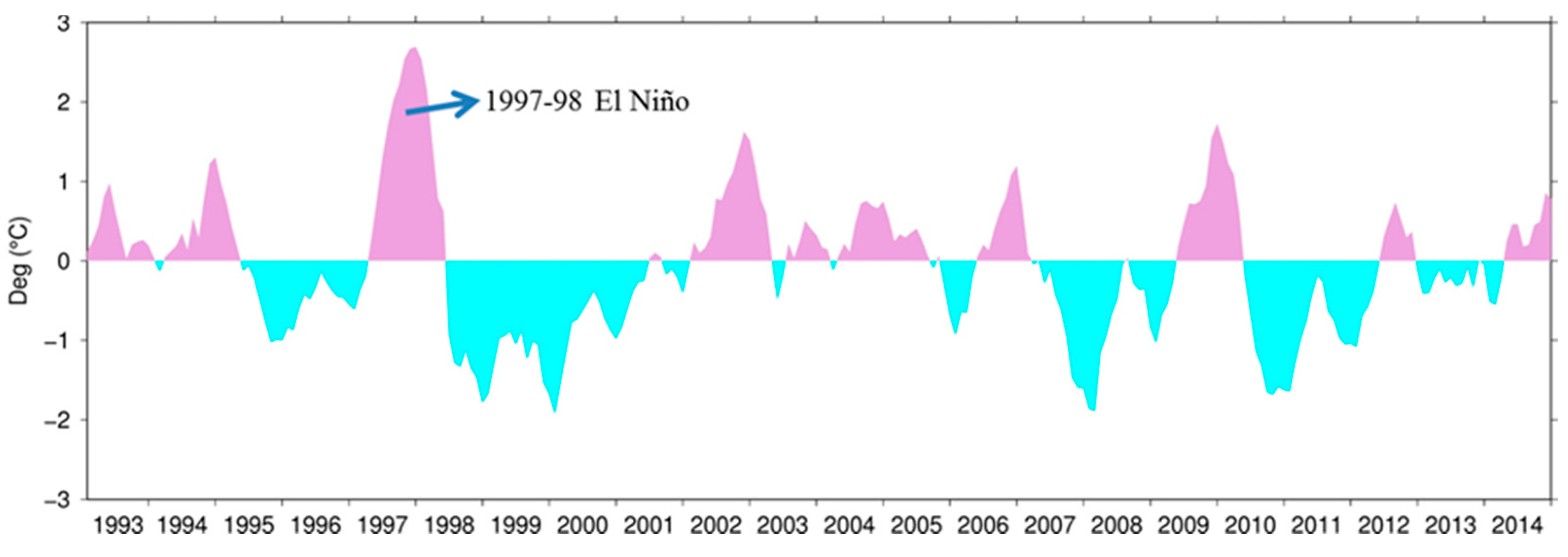
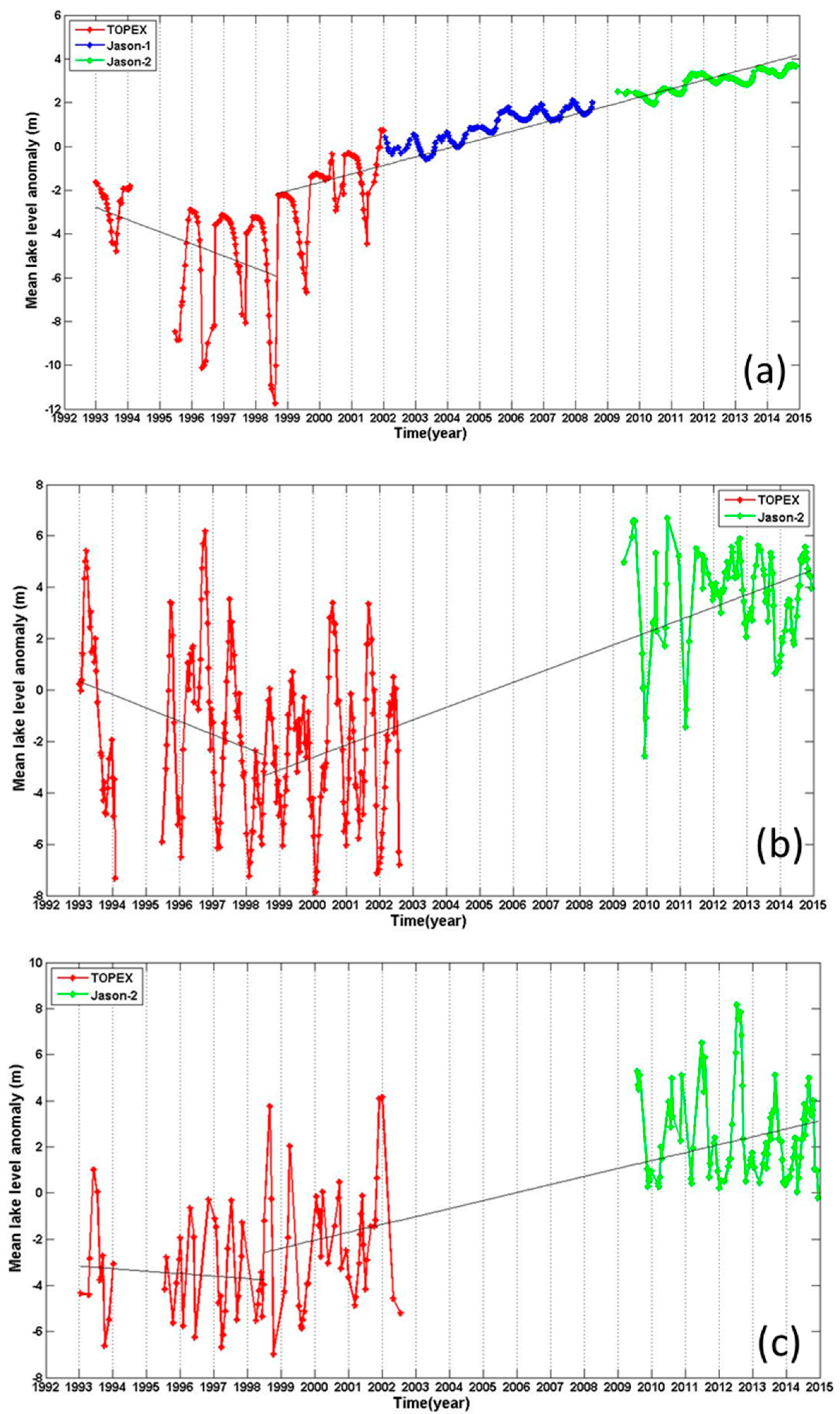
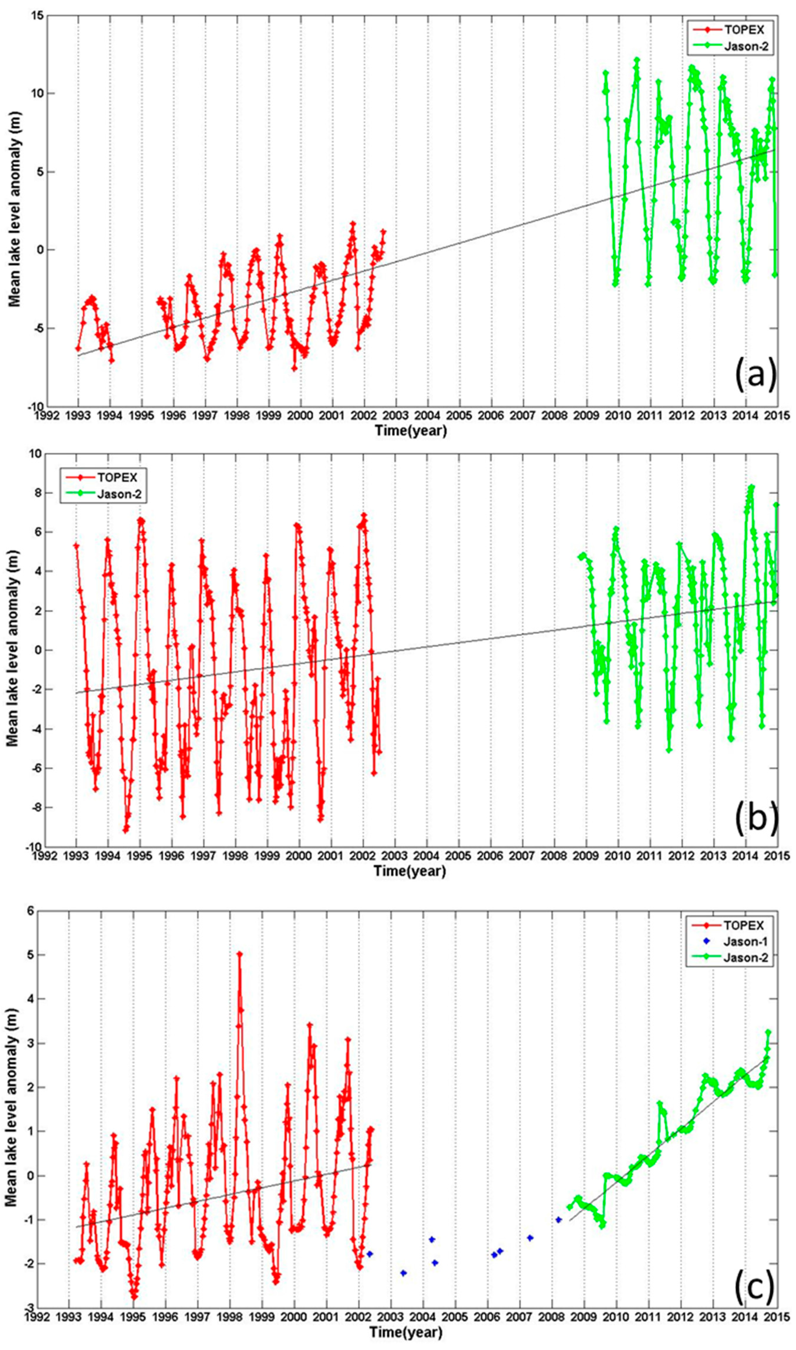
Large annual oscillations occurred before the 1997–1998 El Niño. With the lake level beginning to rise since June 1998, the amplitude of oscillation decreased. This indicates that a smaller lake body (before June 1998) is more sensitive to water influx change than a larger body (after June 1998). The lake level lows vary from May to June, indicating different onset times of snow melting. The most striking feature is: the highs consistently occurred in December over January 1993–December 2014.
(2)
Lake levels at Dagze Co and Gyarab Co underwent large annual oscillations before and after the 1997–1998 El Niño. In comparison to Ngangzi, the lake level highs occurred in autumn and the lows in early spring.
(II) 
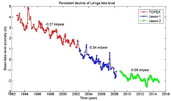
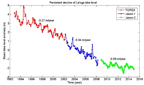
Lakes with continuous dropping trends—La’nga (No. 22), Zhapu (No. 23), and Margog Caka (No. 11)
Figure 8 shows three lakes with continuous dropping trends: La’nga Co (Figure 8a), Zhapu Co (Figure 8b), and Margog Caka (Figure 8c). La’nga Co is located in the interior of Tibet and is adjacent to its sister lake, Mapam. T/P passes through the deepest part of this lake, delivering good waveforms for further improvement by the subwaveform retracking. Over January 1993–December 2014, the mean rate of lake level change here is −0.30 m/year. However, the rate varies with time: over 1993–2002, 2002–2008, and 2009–2014, the rates are −0.27, −0.34 and −0.09 m/year, respectively. Seasonal lake level oscillations are evident, with the lows and highs in December and August.
At Zhapu Co, the observations from J1 are sparse. The T/P and J2 results show a mean rate of −0.04 m/year and clear annual oscillations, with the highs in December and the lows in June-July. At Margog Caka, no J1 and J2 observations are available. The T/P observations show a continuous, steady rate of about −0.47 m/year over January 1993–August 2002. Despite Margog Caka’s steady declining rate, the annual peaks of lake oscillations are not regular; there can be two peaks in a year and the lows can be in summer and winter.
(III) 
Lakes with continuous rising trends—Zhangnai (No. 13), Zige (No. 5), and Chibuzhang (No. 6)
Figure 9 shows three lakes with continuous rising level. Zhangnai Co (Figure 9a) is located in Nagqu of Tibet with water mainly from runoffs. The highs and lows of lake level occurred in summer and winter. Over January 1993–December 2014, the mean rising rate is 0.60 m/year. Over 1993–2000, the rate decreased to 0.28 m/year, with peaks of lake level oscillations up to 5 m. There is no J1 observation at Zhangnai Co. Over January 2009–December 2014, J2-observed lake levels are about 10 m higher than the mean lake levels from T/P over 1993–2000. From 2009 to 2014, the rising rate became more moderate at 0.1 m/year, but the peaks of height oscillations reached 15 m.
Zige Co (Figure 9b) receives water mainly from precipitation and runoff. Without any glacier in its catchment area, the lake level is not affected by glacier melting. Like Zhangnai Co, there is no J1 observation at Zige Co over January 2002–December 2008. From January 1993 to December 2003, the rising rate is 0.14 m/year, accelerating to 0.30 m/year over 2009–2014. From January 1993 to December 2014, the mean rising rate is 0.21 m/year. The annual oscillations are evident with the highs and lows in winter and summer. According to Huang et al. [4], the rising rates of Zige Co’s lake area over 1990–2000 and 2000–2010 are 0.30 and 2.02 km2/year, respectively. These rising trends in lake area are consistent with rising trends in lake level observed by T/P and J2.
Chibuzhang Co (Figure 9c) receives water mainly from melted snow of Mt. Tanggula and surface runoff [1]. The lake level is high in summer and low in winter. Here J1 provided only few observations over January 2002–December 2008. The annual oscillations over 1993–2000 are significantly larger than the oscillations over 2008–2014. The highs over 2008–2014 occurred between late summer and autumn, compared to the highs over 1993–2000 that typically occurred in May-June. In May 1998, there was a sharp increase in the annual high. Notably are the changes of rate: the rate is 0.16 m/year over 1993–2002, increasing to 0.61 m/year over 2008–2014. The latter is almost four times of the former. The fast increase of Chibuzhang Co lake level over 2008–2014 could be partially attributed to the rapid, negative glacier mass balance around Mt. Tanggula [47]. Moreover, increased precipitations can also contribute to the accelerating rate of lake level rise at Chibuzhang Co (see Section 5.1 for more details).
In June 1999, unexpectedly there was no annual high at Chibuzhang Co, compared to other years. This indicates that there was a deficit in precipitation or melting snow from Mt. Tanggula, or both. It is likely that this anomalous pattern of high and low in 1998–1999 is due to the 1997–1998 El Niño. It is well known that Chibuzhang Co receives most water from mountain glaciers [1]. In this case, it might be possible to use changes in lake level and lake area to infer the mass loss at the source area of the lake, namely glaciers of Mt. Tanggula, provided that constraints on regional precipitation, runoff and evaporation are available.

5. Discussions

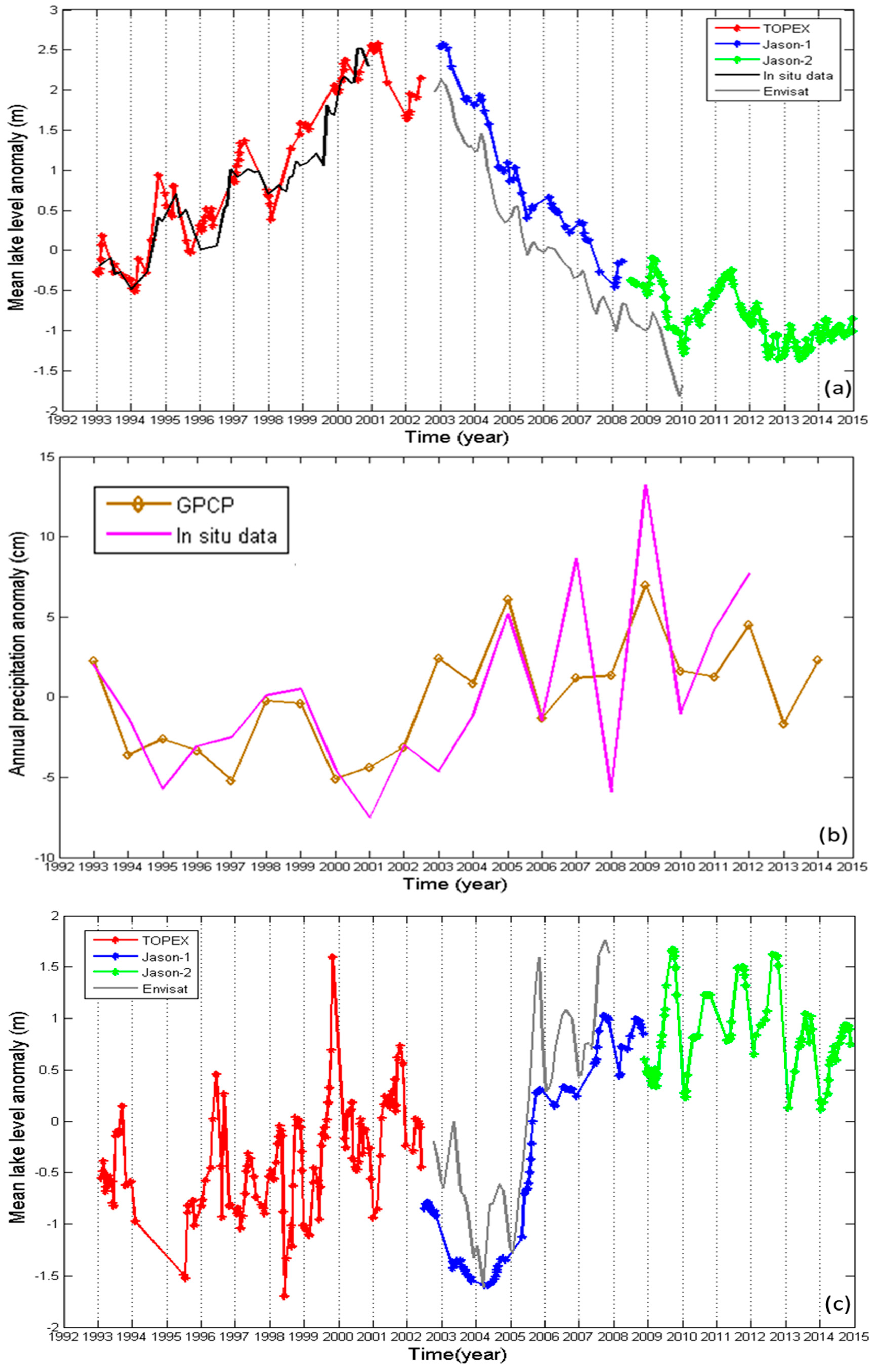
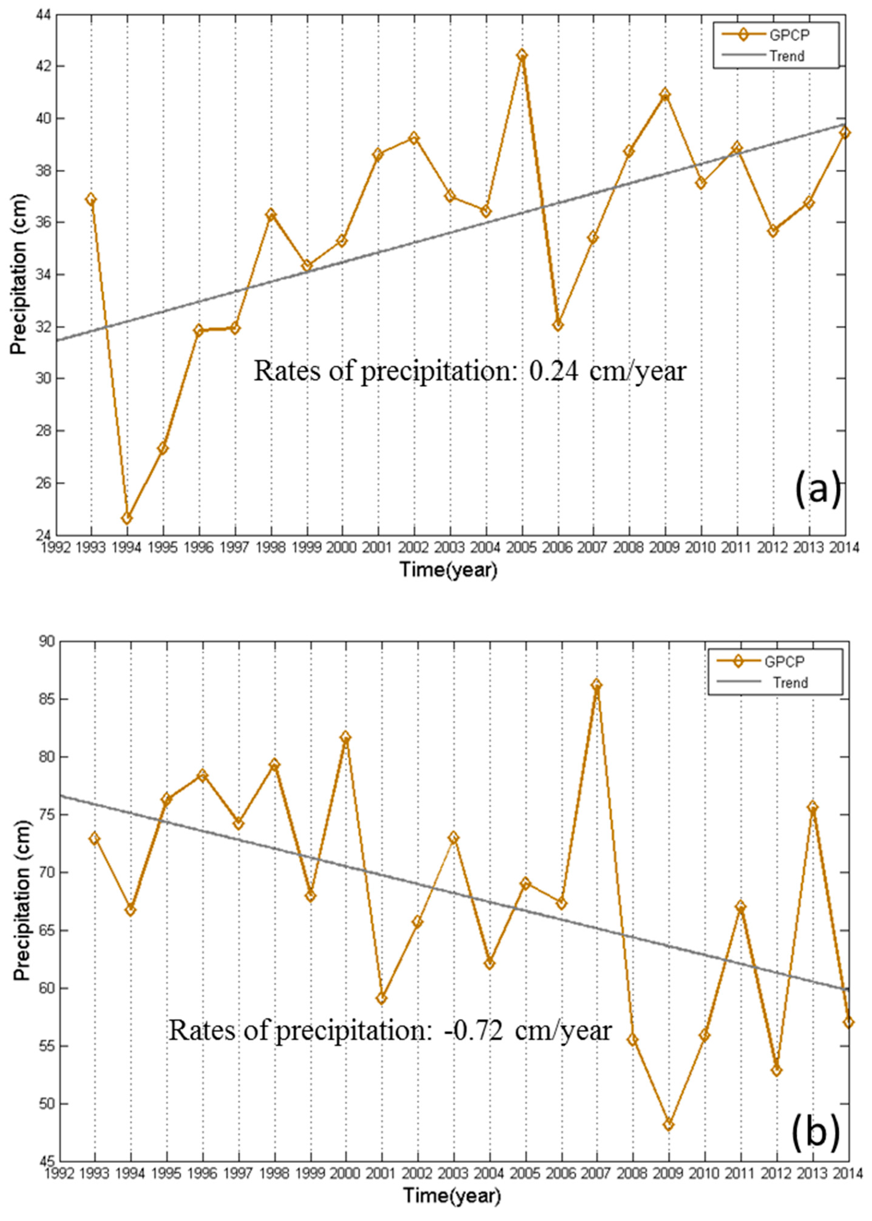
5.1. Lakes with Steady Lake Trends: Contribution of Precipitation

In Section 4, we show the general pattern of lake level rate and selected lake level time series, and point out the connection between the rates of lake level and the rates of precipitation. The lakes with the same feature of lake level change are basically close geographically, and are related to their locations in Tibet that have different extents of influences by the Indian monsoon, East Asian monsoon and westerlies. To expand the discussion in Section 4, Figure 10 shows the trends of annual cumulative precipitations from GPCP at the centers of La’nga Co (continuous falling lake level) and Chibuzhang Co (continuous rising lake level). The precipitations at La’nga Co declined steadily over January 1993–December 2014, slowing down between 2009 and 2014. In contrast, at Chibuzhang Co, there is a sharp decrease of precipitation in 1994, followed by rises between 1994 and 2001. In summary, the GPCP-derived precipitation trends are coherent with the trends of lake levels at Chibuzhang Co and La’nga Co, and can partially explain the latter.

5.2. Inter-Altimeter Bias and Adding ERS-Family Satellites to Increase Lake Coverage

An important condition for a reliable, long-term lake level time series from T/P, J1 and J2 is that there are no inter-satellite biases among them. From the time series plots presented in this paper (Figure 4, Figure 5, Figure 6, Figure 7, Figure 8 and Figure 9), it seems there are no apparent biases among the three TP-family satellites. However, inter-satellite biases are geographically dependent [48] and there are no papers reporting such biases in the QTP. Whether such biases exist and how they might disrupt the T/P-J2 lake level time series over the 23 lakes remain unclear. Therefore, we suggest that previous studies on the T/P- J1-J2 biases [48] should be re-visited, particularly over land mass. In addition, the ongoing J3 mission can use measurements at the J2-J3 overlapping arcs over Tibet to investigate potential biases between the two satellites.
Another issue is lake level monitoring in the QTP using the ERS-family satellites, including ERS-1, ERS-2 and Envisat. These satellites have a repeat period of 35 days, making their cross-track distances much smaller than T/P’s, and allowing the satellites to observe more lakes than T/P in the QTP. In Section 4.2, we have shown lake level changes at Bosten Lake and Eling Lake from Envisat. The lake level time series at these two lakes from Envisat and J1 are consistent in both annual oscillation and trend. The combination of altimeter data from ERS-1, ERS-2, Envisat and the ongoing Sentinel-3 altimeter will yield lake level changes in the QTP every 35 days with a dense coverage. In addition, the joint India-France altimeter mission SARAL (launched on 25 February 2013) covers the same ground tracks of Envisat. SARAL uses a Ka-band altimeter (ALTIKA) for ranging and will have a smaller footprint size than the Ku-band altimeters in the T/P-family satellites. SARAL may also contribute to lake level change studies, but there is no document reporting SARAL’s data quality and availability in the QTP. Potential biases between the T/P-family and ERS-family altimeters should also be examined for coherent time series of lake level change.

5.3. Advantage of Radar Altimeter: Not Only Laser Altimeter Is Needed

A final discussion is on the comparison of lake level monitoring by radar altimeters and by laser altimeters. The strength of a laser altimeter such as ICESat is its wide spatial coverage, small footprint size and higher ranging accuracy. Perhaps ICESat’s only weakness is its coarse temporal resolution that can yield aliased signals in lake level change. For example, a small lake may contain ICESat measurements only in summer or winter, making it not possible to see seasonal oscillations and trends. Most radar altimeters are designed to observe sea level change and icesheet mass balance, so they have repeat ground tracks. As stated in Section 1, repeat ground tracks allow short temporal resolutions. If a lake is lucky to contain one or two repeat ground tracks, the state of its lake level can be monitored as long as the sea level monitoring program lasts.

6. Conclusions

In this paper, we determined lake level time series at 23 lakes in the QTP along repeat tracks of T/P-family satellites over January 1993–December 2014. The number of lakes is far less than the numbers of ICESat-detected lakes reported in Zhang et al. [1], Song et al. [11], and Phan et al. [49,50]. However, these time series have a short sampling interval of 10 days, compared to the longer, unevenly sample intervals of ICESat. For example, at Ngangzi Co, J1 delivered 180 repeat height measurements over 2003–2008, while ICESat delivered only 16 repeat measurements during this period [1]. The 23 lakes are optimal lakes in the QTP for long-term monitoring of lake level by the T/P-family satellites beyond the mission J3. Long-term lake level records at the 23 lakes that can be used to study the impact of climate change on lake level change in the QTP. In addition, the T/P-family satellites can also detect sudden lake level changes to help predictions of lake outbursts and provide warnings of potential flooding in the lake’s downstream (see the example of Kusai Lake, Section 4.2).
From January 1993 to December 2014, the overall trend of lake level in eastern Tibet is positive, while the average trend is western Tibet is negative. These contrasting rates may be caused by the variations in the Indian monsoon, the East Asia monsoon and the westerlies, but exactly how remains unclear. In central Tibet, lake level trends at Ngangzi Co, Dagze Co, and Gyarab Co were negative before the 1997-98 El Niño and turned to positive after this event. Some lakes see continuously rising and falling trends, and are positively correlated with the trends of precipitation. At some lakes, the amplitudes of annual oscillations vary with time, reflecting the changes of the lake’s volumes and the change in raining pattern. Finally, we suggest a combined use of the T/P-family and ERS-family satellites that will yield unprecedented temporal and spatial resolutions for lake monitoring in the QTP, provided that inter-satellite biases are properly modeled.

Acknowledgments

We are grateful to AVISO for the altimeter data. This study is supported by Ministry of Science and Technology, Taiwan, under Grants 103-2221-E-009-114-MY3 and 104-2611-M-009-001, and NSFC (China) under Grant 41429401.

Author Contributions

C.H. initiated the study and wrote the first draft. All authors carried out the computations and analyses, and wrote the final draft.

Conflicts of Interest

The authors declare no conflict of interest.

References

  1. Zhang, G.; Xie, H.; Kang, S.; Yi, D.; Ackley, S.F. Monitoring lake level changes on the Tibetan Plateau using ICESat altimetry data (2003–2009). Remote Sens. Environ. 2011, 115, 1733–1742. [Google Scholar] [CrossRef]
  2. Li, L.; Wang, W. The response of lake change to climate fluctuation in north Qinghai-Tibet Plateau in last 30 years. J. Geog. Sci. 2009, 19, 131–142. [Google Scholar]
  3. Liu, X.; Chen, B. Climatic warming in the Tibetan Plateau during recent decades. Int. J. Climatol. 2000, 20, 1729–1742. [Google Scholar] [CrossRef]
  4. Huang, W.; Liao, J.; Shen, G. Lake change in past 40 years in the southern Nagqu District of Tibet and analysis of its driving forces. Remote Sens. Land Resour. 2012, 24, 122–128. (In Chinese) [Google Scholar]
  5. Qiu, J. The third pole. Nature 2008, 454, 393–396. [Google Scholar] [CrossRef] [PubMed]
  6. Shao, Z.; Zhu, D.; Meng, X.; Zheng, D.; Qiao, Z.; Yang, C.; Han, J.; Yu, J.; Meng, Q.; Lü, R. Characteristics of the change of major lakes on the Qinghai-Tibet Plateau in the last 25 years. Front. Earth Sci. China 2008, 2, 364–377. [Google Scholar] [CrossRef]
  7. Yao, X.; Liu, S.; Li, L.; Sun, M.; Luo, J. Spatial-Temporal characteristics of lake area variations in Hoh Xil region from 1970 to 2011. J. Geograph. Sci. 2014, 24, 689–702. [Google Scholar] [CrossRef]
  8. Morris, C.S.; Gill, S.K. Evaluation of the TOPEX/POSEIDON altimeter system over the Great Lakes. J. Geophys. Res. 1994, 99, 24527–24539. [Google Scholar] [CrossRef]
  9. Alsdorf, D.; Birkett, C.; Dunne, T.; Melack, J.; Hess, L. Water level changes in a large Amazon lake measured with space borne radar interferometry and altimetry. Geophys. Res. Lett. 2001, 28, 2671–2674. [Google Scholar] [CrossRef]
  10. Hwang, C.; Peng, M.F.; Ning, J.; Luo, J.; Sui, C.H. Lake level variations in China from TOPEX/Poseidon altimetry: Data quality assessment and links to precipitation and ENSO. Geophys. J. Int. 2005, 161, 1–11. [Google Scholar] [CrossRef]
  11. Song, C.; Huang, B.; Ke, L.; Richards, K.S. Seasonal and abrupt changes in the water level of closed lakes on the Tibetan Plateau and implications for climate impacts. J. Hydrol. 2014, 514, 131–144. [Google Scholar] [CrossRef]
  12. Kleinherenbrink, M.; Lindenbergh, R.C.; Ditmar, P.G. Monitoring of lake level changes on the Tibetan Plateau and Tian Shan by retracking Cryosat SARIn waveforms. J. Hydrol. 2015, 521, 119–131. [Google Scholar] [CrossRef]
  13. Aviso User Handbook—Merged TOPEX/POSEIDON Products (GDR-Ms). Available online: http://www.aviso.altimetry.fr/fileadmin/documents/data/tools/hdbk_tp_gdrm.pdf (accessed on 22 May 2016).
  14. OSTM/Jason-1 Products Handbook. Available online: http://www.aviso.altimetry.fr/fileadmin/documents/data/tools/hdbk_j1_gdr.pdf (accessed on 22 May 2016).
  15. OSTM/Jason-2 Products Handbook. Available online: http://www.aviso.altimetry.fr/fileadmin/documents/data/tools/hdbk_j2.pdf (accessed on 22 May 2016).
  16. French space agency AVISO. Available online: http://www.aviso.altimetry.fr/ (accessed on 22 May 2016).
  17. Frappart, F.; Calmant, S.; Cauhopé, M.; Seyler, F.; Cazenave, A. Preliminary results of ENVISAT RA-2-derived water levels validation over the Amazon basin. Remote Sens. Environ. 2006, 100, 252–264. [Google Scholar] [CrossRef] [Green Version]
  18. Yan, L.; Zheng, M. The response of lake variations to climate change in the past forty years: A case study of the northeastern Tibetan Plateau and adjacent areas, China. Quat. Int. 2015, 371, 31–48. [Google Scholar] [CrossRef]
  19. Zhu, D.; Zhao, X.; Meng, X.; Wu, Z.; Shao, Z.; Ma, Z.; Yang, Z.; Wang, J. Lake-Level fluctuation of Nam Co, Tibet, since the late Pleistocene, and evolution of an ancient large lake on the northern Tibetan Plateau. Geol. Bull. China 2003, 22, 918–927. (In Chinese) [Google Scholar]
  20. Yan, L.; Zheng, M. Influence of climate change on saline lakes of the Tibet Plateau, 1973–2010. Geomorphology 2015, 246, 68–78. [Google Scholar] [CrossRef]
  21. Zheng, M. An Introduction to Saline Lakes on the Qinghai—Tibet Plateau; Kluwer Academic Publishers: Dordrecht, The Netherlands, 1997. [Google Scholar]
  22. Taylor, M.; Yin, A.; Ryerson, F.J.; Kapp, P.; Ding, L. Conjugate strike-slip faulting along the Bangong-Nujiang suture zone accommodates coeval east-west extension and north-south shortening in the interior of the Tibetan Plateau. Tectonics. 2003, 22. [Google Scholar] [CrossRef]
  23. Becker, J.J.; Sandwell, D.T.; Smith, W.H.F.; Braud, J.; Binder, B.; Depner, J.; Fabre, D.; Factor, J.; Ingalls, S.; Kim, S.-H.; et al. Global bathymetry and elevation data at 30 arc seconds resolution: SRTM30_PLUS. Mar. Geod. 2009, 32, 355–371. [Google Scholar] [CrossRef]
  24. Shum, C.; Yi, Y.; Cheng, K.; Kuo, C.; Braun, A.; Calmant, S.; Chambers, D. Calibration of JASON-1 altimeter over lake erie special issue: Jason-1 calibration/validation. Mar. Geod. 2003, 26, 335–354. [Google Scholar] [CrossRef]
  25. Lee, H.K. Radar Altimetry Methods for Solid Earth Geodynamics Studies. Ph.D. Thesis, The Ohio State University, Columbus, OH, USA, 2008. [Google Scholar]
  26. Martin, T.V.; Zwally, H.J.; Brenner, A.C.; Bindschadler, R.A. Analysis and retracking of continental ice sheet radar altimeter waveforms. J. Geophys. Res. 1983, 88, 1608–1616. [Google Scholar] [CrossRef]
  27. Wingham, D.J.; Rapley, C.G.; Griffiths, H. New techniques in satellite altimeter tracking systems. In Proceedings of the 1986 International Geoscience and Remote Sensing Symposium (IGARSS’86) on Remote Sensing: Today’s Solutions for Tomorrow’s Information Needs; ESA Publication Division: Noordwijk, The Netherlands, 1986; Volume 3, pp. 1339–1344. [Google Scholar]
  28. Laxon, S. Sea ice altimeter processing scheme at the EODC. Int. J. Remote Sens. 1994, 15, 915–924. [Google Scholar] [CrossRef]
  29. Davis, C.H. A robust threshold retracking algorithm for measuring ice-sheet surface elevation change from satellite radar altimeters. IEEE Trans. Geosci. Remote Sens. 1997, 35, 974–979. [Google Scholar] [CrossRef]
  30. Hwang, C.; Guo, J.; Deng, X.; Hsu, H.Y.; Liu, Y. Coastal gravity anomalies from retracked Geosat/GM altimetry: Improvement, limitation and the role of airborne gravity data. J. Geod. 2006, 80, 204–216. [Google Scholar] [CrossRef]
  31. Yang, Y.; Hwang, C.; Hsu, H.J.; Dongchen, E.; Wang, H. A subwaveform threshold retracker for ERS-1 altimetry: A case study in the Antarctic Ocean. Comput. Geosci. 2012, 41, 88–98. [Google Scholar] [CrossRef]
  32. Yang, Y.; Hwang, C.; Dongchen, E. A fixed full-matrix method for determining ice sheet height change from satellite altimeter: An ENVISAT case study in East Antarctica with backscatter analysis. J. Geod. 2014, 88, 901–914. [Google Scholar] [CrossRef]
  33. Hsiao, Y.S.; Hwang, C.; Cheng, Y.S.; Chen, L.C.; Hsu, H.J.; Tsai, J.H.; Liu, C.L.; Wang, C.C.; Liu, Y.C.; Kao, Y.C. High-Resolution depth and coastline over major atolls of South China Sea from satellite altimetry and imagery. Remote Sens. Environ. 2016, 176, 69–83. [Google Scholar] [CrossRef]
  34. Brown, G.S. The average impulse response of a rough surface and its applications. IEEE Trans. Antennas Propag. 1977, 25, 67–74. [Google Scholar] [CrossRef]
  35. Dabo-Niang, S.; Ferraty, F.; Vieu, P. On the using of modal curves for radar waveforms classification. Comput. Stat. Data Anal. 2007, 51, 4878–4890. [Google Scholar] [CrossRef]
  36. Yao, T.; Thompson, L.; Yang, W.; Yu, W.; Gao, Y.; Guo, X.; Yang, X.; Duan, K.; Zhao, H.; Xu, B. Different glacier status with atmospheric circulations in Tibetan Plateau and surroundings. Nat. Clim. Chang. 2012, 2, 663–667. [Google Scholar] [CrossRef]
  37. Wang, R.; Giese, E.; Gao, Q.Z. The recent change of water level in the Bosten Lake and analysis of its causes. J. Glaciol. Geocryol. 2003, 25, 60–64. (In Chinese) [Google Scholar]
  38. Wang, R.; Sun, Z.; Gao, Q.Z. Water level change in Bosten Lake under the climate variation background of Central Asian ariund 2002. J. Glaciol. Geocryol. 2006, 28, 324–329. (In Chinese) [Google Scholar]
  39. Menne, M.J.; Durre, I.; Gleason, B.G.; Houston, T.G.; Vose, R.S. An overview of the global historical climatology network-daily database. J. Atmos. Ocean. Technol. 2012, 29, 897–910. [Google Scholar] [CrossRef]
  40. Hu, Y.; Maskey, S.; Uhlenbrook, S.; Zhao, H. Streamflow trends and climate linkages in the source region of the Yellow River, China. Hydrol. Process. 2011, 25, 3399–3411. [Google Scholar] [CrossRef]
  41. Guangming Online, Ideology and Culture in China. Available online: http://epaper.gmw.cn/gmrb/html/2013-08/04/nbs.D110000gmrb_03.htm/ (accessed on 22 May 2016).
  42. Administrative Bureau of Hoh Xil National Nature Reserve. Available online: http://www.kkxl.org.cn/ (accessed on 22 May 2016).
  43. Xiaojun, Y.; Shiyin, L.; Meiping, S. Changes of Kusai Lake in Hoh Xil region and causes of its water overflowing. Acta Geograph. Sin. 2012, 67, 689–698. (In Chinese) [Google Scholar]
  44. Fujita, K.; Sakai, A.; Takenaka, S.; Nuimura, T.; Surazakov, A.B.; Sawagaki, T.; Yamanokuchi, T. Potential flood volume of Himalayan glacial lakes. Nat. Hazards Earth Syst. Sci. 2013, 13, 1827–1839. [Google Scholar] [CrossRef]
  45. Liu, J.J.; Cheng, Z.L.; Li, Y. The 1988 glacial lake outburst flood in Guangxieco Lake, Tibet, China. Nat. Hazard. Earth Syst. 2014, 14, 3065–3075. [Google Scholar] [CrossRef]
  46. Niño 3.4 SST Index. Available online: http://www.esrl.noaa.gov/psd/gcos_wgsp/Timeseries/Nino34/ (accessed on 22 May 2016).
  47. Pu, J.C.; Yao, T.D.; Yang, M.X.; Tian, L.D.; Wang, N.L.; Ageta, Y.; Fujita, K. Rapid decrease of mass balance observed in the Xiao (Lesser) Dongkemadi Glacier, in the central Tibetan Plateau. Hydrol. Process. 2008, 22, 2953–2958. [Google Scholar] [CrossRef]
  48. Fu, L.L.; Haines, B.J. The challenges in long-term altimetry calibration for addressing the problem of global sea level change. Adv. Space Res. 2013, 51, 1284–1300. [Google Scholar] [CrossRef]
  49. Phan, V.H.; Lindenbergh, R.; Menenti, M. ICESat derived elevation changes of Tibetan lakes between 2003 and 2009. Int. J. Appl. Earth Observ. Geoinform. 2012, 17, 12–22. [Google Scholar] [CrossRef]
  50. Phan, V.H.; Lindenbergh, R.; Menenti, M. Seasonal trends in Tibetan lake level changes as observed by ICESat laser altimetry. ISPRS Int. Ann. Photogramm. Remote Sens. Spat. Inf. Sci. 2012, 1, 237–242. [Google Scholar] [CrossRef]
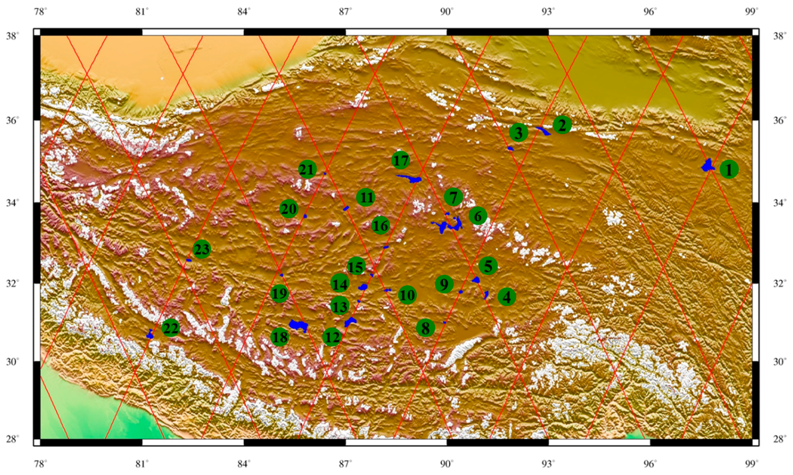
Figure 1. The locations and dimensions of the 23 lakes (blue-shaded) in the QTP observed by the T/P-family satellites. The red lines denote the satellite ground tracks and the numbers represent the lake IDs in Table 1.
Remotesensing 08 00446 g001
Figure 2. Radar waveforms at spots 1–33 around La’nga Co (left-lower corner; No. 22, Figure 1).
Remotesensing 08 00446 g002
Figure 3. (a) Rates of lake level change at 23 lakes from January 1993 to December 2014 with wind directions of westerlies, Indian monsoon and East Asian monsoon; (b) rates of precipitation from GPCP in the same period.
Remotesensing 08 00446 g003
Figure 4. (a) Lake level change at Bosten Lake; (b) GPCP and in situ precipitation from weather station near Eling Lake (No. 1); (c) Lake level change at Eling Lake.
Remotesensing 08 00446 g004
Figure 5. Lake level change at Kusai Lake (No. 2).
Remotesensing 08 00446 g005
Figure 6. The Niño 3.4 index over 1993–2014, showing the large positive temperature anomalies during the 1997–1998 El Niño.
Remotesensing 08 00446 g006
Figure 7. Lake level changes at three lakes showing reversed trends before and after the 1997–1998 El Niño: (a) Ngangzi (No. 12); (b) Dagze (No. 14); and (c) Gyarab (No. 15).
Remotesensing 08 00446 g007
Figure 8. Lake level changes at three lakes showing continuous falling levels: (a) La’nga (No. 22); (b) Zhapu (No. 23); and (c) Margog Caka (No. 11).
Remotesensing 08 00446 g008
Figure 9. Lake level changes at three lakes showing continuous rising levels: (a) Zhangnai (No. 13); (b) Zige (No. 5); and (c) Chibuzhang (No. 6).
Remotesensing 08 00446 g009
Figure 10. Rates of precipitation from GPCP around (a) Chibuzhang Co and (b) La’nga Co.
Remotesensing 08 00446 g010
Table 1. ID numbers, names and other information of the 23 lakes tracked by T/P, J1 and J2 satellite altimeters (see Figure 1).
ID 1Name 2Approximate Longitude, LatitudeArea (km2)TrackApproximate Altitude 3 (m)Reference
1Eling97.68, 34.88610.7216, 0534696[18]
2Kusai92.77, 35.782721555190[18]
3Cuodarima91.85, 35.3389.90644786[18]
4Dong91.12, 31.611232425153[1]
5Zige90.90, 32.062342424579[1]
6Chibuzhang90.09, 33.405202425377[18]
7Laorite89.95, 33.7157.32424729[18]
8Jiuru89.94, 31.0040.41555679[19]
9Dongqia90.40, 31.7946.71555006[20]
10Qagoi88.19, 31.8188.51664841[1]
11Margog Caka87.03, 33.8690.71665043[1]
12Ngangzi87.21, 31.04461.50794471[1]
13Zhangnai87.40, 31.53360795197-
14Dagze87.62, 31.882930794789[1]
15Gyarab87.79, 32.19490794722[11]
16Pongyin88.18, 32.8948.80794680[21]
17Dogai Coring89.13, 34.59393.30795315[1]
18Zhari Nam85.78, 30.93996.90904823[1]
19Zhaxi85.13, 32.2047.20904599[22]
20Gomo85.82, 33.66760035397[21]
21Qingwa86.40, 34.7125.310035218[7]
22La’nga81.22, 30.66268.51815145[10]
23Zhapu82.40, 32.5657.91814550-
1 ID number in Figure 1; 2 Lake is sometimes called “Co” in Tibetan; either “lake” or “Co” is omitted here; 3 The altitude is interpolated from the SRTM-plus DEM [23].
Table 2. Rates of lake level change (in m/year) from TOPEX/Poseidon (1993–2002) and Jason-2 (2008–2014).
ID1LakeTOPEX/PoseidonJason-2
1Eling0.07 ± 0.01−0.03 ± 0.01
2Kusai0.47 ± 0.141.58 ± 0.08
3Cuodarima−0.13 ± 0.050.51 ± 0.03
4Dong0.16 ± 0.030.61 ± 0.01
5Zige0.05 ± 0.080.12 ± 0.12
6Chibuzhang0.15 ± 0.050.30 ± 0.08
7Laorite0.09 ± 0.07−0.02 ± 0.02
8Jiuru0.21 ± 0.060.02 ± 0.01
9Dongqia−0.34 ± 0.08−0.08 ± 0.02
10Qagoi0.28 ± 0.110.02 ± 0.02
11Margog Caka−0.47 ± 0.03−2.63 ± 0.8
12Ngangzi0.35 ± 0.050.25 ± 0.01
13Zhangnai0.28 ± 0.04−0.10 ± 0.12
14Dagze−0.31 ± 0.060.08 ± 0.09
15Gyarab0.24 ± 0.1−0.08 ± 0.08
16Pongyin0.10 ± 0.18-0.14 ± 0.13
17Dogai Coring0.11 ± 0.050.91 ± 0.16
18Zhari Nam0.36 ± 0.01−2.05 ± 0.77
19Zhaxi-0.33 ± 0.05
20Gomo0.22 ± 0.060.26 ± 0.16
21Qingwa0.00 ± 0.02-
22La’nga−0.27 ± 0.01−0.09 ± 0.01
23Zhapu−0.02 ± 0.03−0.09 ± 0.03

