1. Introduction
The Earth’s satellite observation systems have been used in various geoscience studies of the Earth’s interior and processes. The global elevation models derived from processing the Shuttle Radar Topography Mission (SRTM) data are used, for instance, to compute the topographic gravity correction in context of the gravimetric interpretation of sedimentary basins as well as other subsurface density structures and/or density interfaces. Apart from climatic studies, the satellite-altimetry observations are also used to determine the marine gravity data. Since the marine gravity field is highly spatially correlated with the ocean-floor relief at a certain wavelength-band, these gravity data are used to predict the ocean-floor depths [
1,
2,
3]. By analogy with applying the topographic gravity correction, the ocean-floor depths are used to compute the bathymetric-stripping gravity correction. The satellite-gravity observations have also been used to interpret the Earth’s inner structure. This becomes particularly possible with the advent of three dedicated satellite-gravity missions, namely the Challenging Mini-satellite Payload (CHAMP) [
4,
5,
6], the Gravity Recovery and Climate Experiment (GRACE) [
7] and the Gravity field and steady-state Ocean Circulation Explorer (GOCE) [
8,
9]. The latest gravitational models derived from these satellite missions have a spatial resolution about 66 to 80 km (in terms of a half-wavelength). Moreover, these gravitational models have (almost) global and homogeneous coverage with well-defined stochastic properties.
Methods for a gravimetric Moho recovery from topographic, bathymetric, gravitational and crustal structure models have been developed and applied by a number of authors (e.g., [
10,
11,
12,
13,
14,
15,
16,
17]). In these studies, a uniform Moho density contrast has often been assumed. The results of seismic studies, however, revealed that the Moho density contrast varies significantly. The continental Moho density contrast 200 kg·m
−3 in Canada was reported by [
18]. Regional seismic studies [
19,
20] based on using the wave-receiver functions indicate that the density contrast regionally varies as much as from 160 kg·m
−3 (for the mafic lower crust) to 440 kg·m
−3 (for the felsic lower crust), with an apparently typical value 440 kg·m
−3 for the craton. The Moho density contrast information is also included in the global crustal model CRUST1.0 [
21]. According to this seismic model, the Moho density contrast (computed as the density difference between the upper mantle and the lower crust) globally varies between 10 and 610 kg·m
−3, while this range is between 340 and 790 kg·m
−3 when computed with respect to the reference crustal density 2670 kg·m
−3 (as often used in gravimetric studies).
An attempt to incorporate the variable Moho density contrast in gravimetric methods for a determination of the Moho depth has been done by some authors. [
22] took into consideration the lateral as well as radial density variation within the crystalline crustal layers and simultaneously adjusted all the densities and estimated the Moho depth. A method for a simultaneous determination of the Moho depth and density contrast developed by [
23] was based on solving the Vening Meinesz-Moritz’s (VMM) inverse problem of isostasy [
24,
25,
26,
27]. This method was applied to estimate the Moho parameters globally and regionally (e.g., [
28]). It was also demonstrated that the gravimetric determination of the Moho depth is more accurate when using the variable Moho density contrast [
29]. The gravimetric results confirmed large variations of the Moho density contrast. According to [
23], the Moho density contrast varies globally from 81.5 kg·m
−3 (in the Pacific region) to 988 kg·m
−3 (beneath the Tibetan Plateau). A similar range of values between 82 and 965 kg·m
−3 was reported by [
30]. It was also shown [
31] that the Moho density contrast under the oceanic crust is highly spatially correlated with the ocean-floor age.
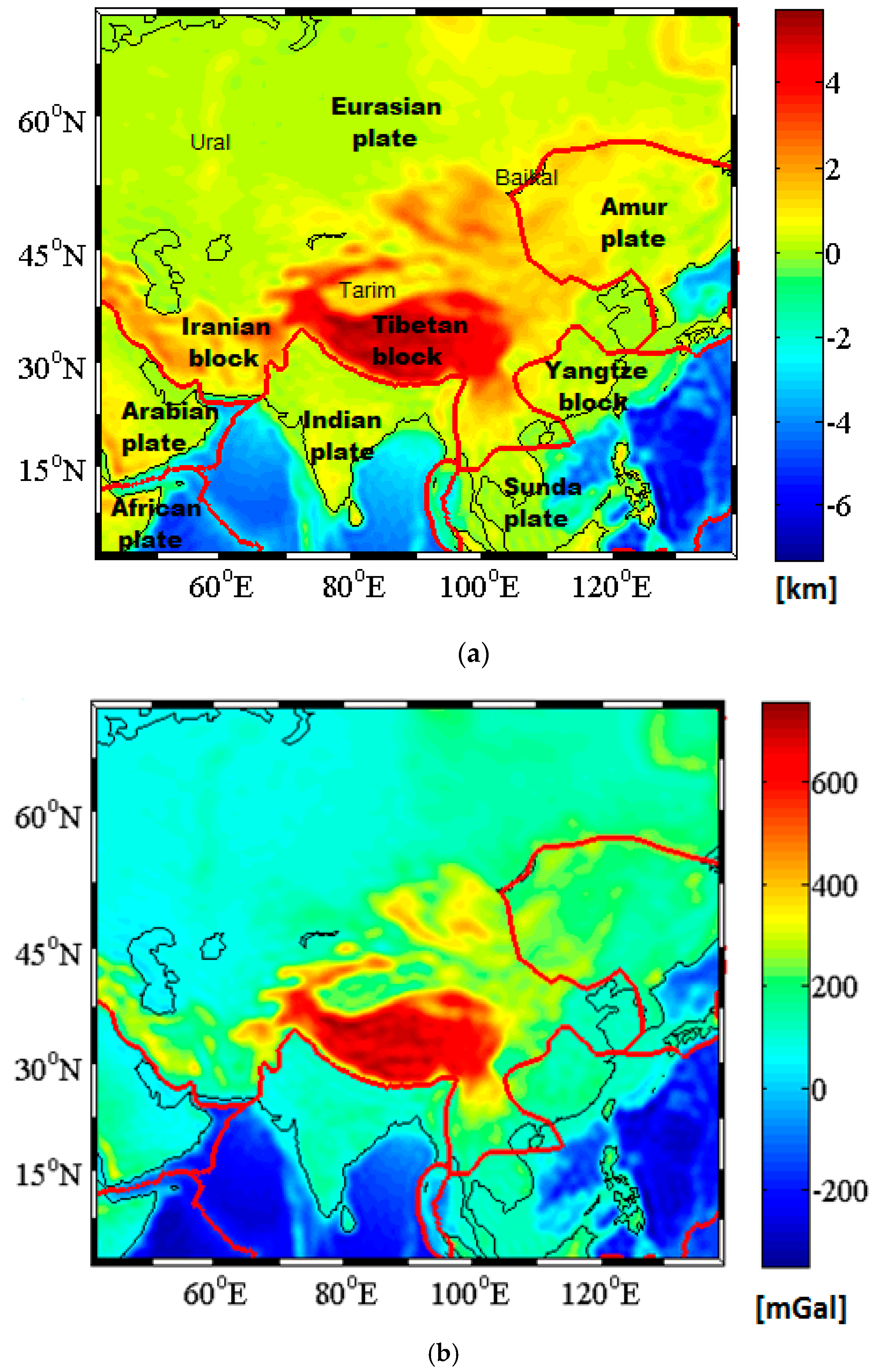
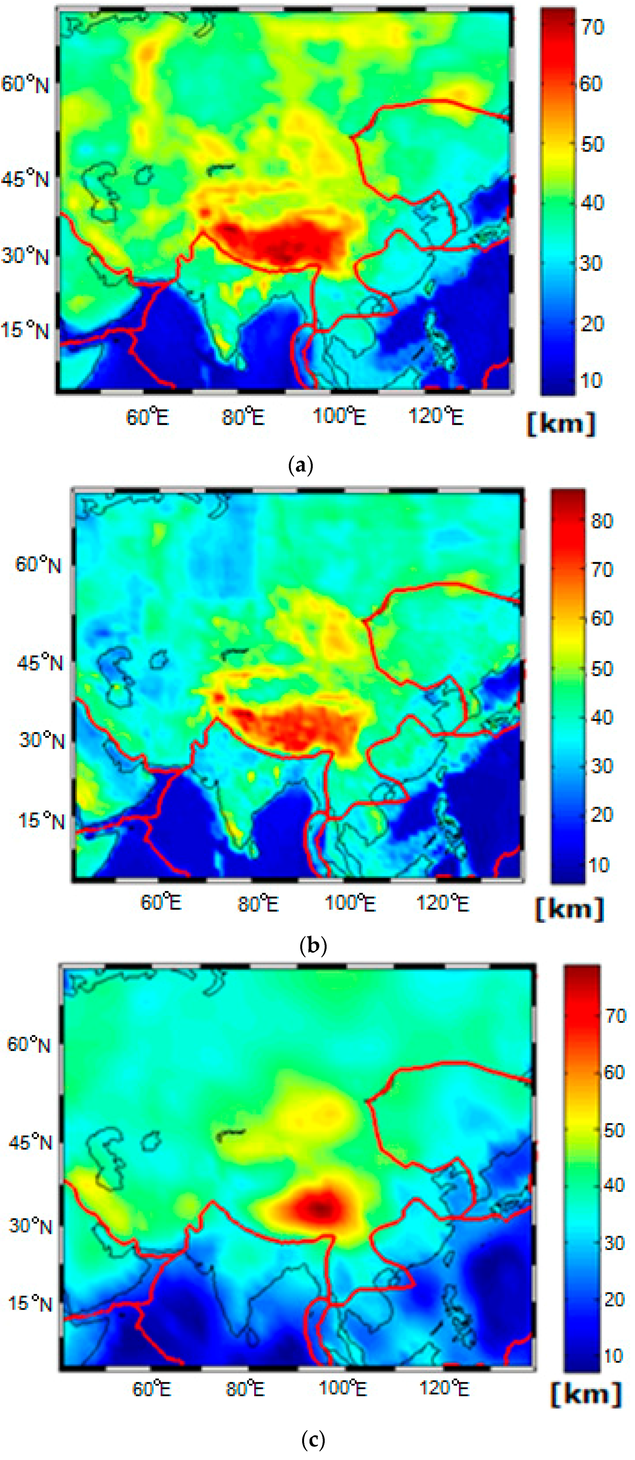
The gravimetrically-determined Moho density contrast [
23,
30] differs significantly from the CRUST1.0 values especially under major orogens in central Asia. To examine this aspect, we investigated the Moho density contrast at the study area which comprises most of the Eurasian tectonic plate and includes also surrounding oceanic and continental plates. For this purpose, we developed and applied a novel approach which utilizes a least-squares technique for solving the condition equations based on minimizing residuals between the gravimetric and seismic Moho parameters, particularly specified for a product of the Moho depth and density contrast.
2. Method
A functional relation between the refined gravity data and the Moho density contrast is defined here by means of solving the VMM inverse problem of isostasy. We note that this functional relation was already derived by [
26], but using a slightly different approach than that presented here. We further extend this definition for finding the Moho density contrast from the in-orbit GOCE gravity-gradient data. We then propose a least-squares technique for solving the VMM problem based on combining the vertical gravity gradients and seismic model and finally investigate a spatial behavior of the integral kernel used for a regional gravity-gradient data inversion.
2.1. Moho Density Contrast from Gravity Disturbance
The VMM isostatic problem was formulated in the following generic form [
26,
27,
32]
where
G is the Newton’s gravitational constant,
R is the Earth’s mean radius,
is the (variable) Moho density contrast,
T is the Moho depth,
is the isostatic gravity disturbance,
σ is the unit sphere, and
is the surface integration element. The integral kernel
K in Equation (1) is a function of the spherical distance
ψ and the Moho depth
T. Its spectral representation reads [
26]
where
Pn is the Legendre polynomial of degree
n.
The isostatic gravity disturbances
on the right-hand side of Equation (1) are computed from the gravity disturbances
by subtracting the gravitational contributions of topography
, bathymetry
and sediments
and adding the compensation attraction
. Hence
The compensation attraction
in Equation (3) is computed from [
26]
where
and
are mean values of the Moho depth and density contrast respectively.
To solve the VMM problem for finding the Moho density contrast
, we first simplified the integral kernel
K in Equation (2). By applying a Taylor series (up to a first-order term) to
, we get
Substitution from Equation (5) to Equation (1) then yields
The surface integral on the left-hand side of Equation (6) is defined in terms of the Laplace harmonic
as follows [
33]
Inserting from Equation (7) to Equation (6), we obtained the following relation
The coefficients
in Equation (8) are generated from the Laplace harmonics
of the isostatic gravity field as follows
where
,
and
are, respectively, the Laplace harmonics of the topographic, bathymetric and sediment gravitational contributions, and
is Kronecker’s delta.
The expression in Equation (9) is finally rearranged into the following form
As seen in Equation (10), the gravity disturbances and gravity corrections are computed in the spectral domain, while the compensation attraction is computed approximately according to Equation (4) from the a priori values of the Moho depth and density contrast.
2.2. Moho Density Contrast from Gravity Gradient
The functional model for finding the Moho density contrast in Equation (10) is now redefined for the vertical gravity gradient (i.e., the second-order radial derivative of the disturbing potential ). It is worth mentioning that results (not presented here) revealed that the contribution of horizontal gravity-gradient components on the Moho parameters is completely negligible.
The relation between the Laplace harmonics
and
reads
where
r is the geocentric radius. The application of a scaling factor
r/
R in Equation (11) allows solving the VMM problem for the gravity-gradient data at an arbitrary point on or above the geoid. Note that the generic expression in Equation (1) defines the VMM problem only on the geoid surface (approximated by a sphere of radius
R). The downward continuation of gravity data observed at the topographic surface (or satellite altitudes) onto the geoid is then required
in prior of solving the VMM problem.
Substitution from Equation (11) to Equation (10) yields
where the parameter
W is defined by
The Laplace harmonics
of the parameter
W are generated from the respective harmonics
of the vertical gravity gradient
using the following expression
Alternatively, the Laplace harmonics
can be defined in the following form [
33]
Substituting from Equation (15) back to Equation (14) and applying further simplifications, we arrived at
where the integral kernel
L reads
A practical computation of the Moho density contrast is realized in two numerical steps. The unknown parameters W are first computed by solving the inverse to the system of observation equations. These observation equations are formed by applying a discretization to the integral equation in Equation (16). The estimated parameters W are then used to compute the Moho density contrast according to the definition given in Equation (12).
2.3. Combined Model
The functional model from Equation (16) is now used to formulate a method for finding the Moho density contrast by combining the gravity-gradient data and seismic crustal model. For this purpose we use the a priori information on the Moho depth and density contrast from an available seismic crustal model to define the condition equation for solving the VMM problem. A least-squares technique is then applied to estimate the Moho density contrast from the gravity-gradient data. Since the accuracy of seismic data is typically not provided, we do not apply a stochastic model.
The condition equation is defined in the following form
where the parameter
M is defined by
The condition equation in Equation (18) assumes that the differences (
i.e., residuals) between the gravimetric and seismic Moho parameters are minimized by means of applying a least-squares technique. The system of condition equations then becomes
and
The system of condition equations can uniquely be solved by applying the minimum-norm condition. Hence, we have
The solution of Equation (22) yields the correction terms to the Moho parameters.
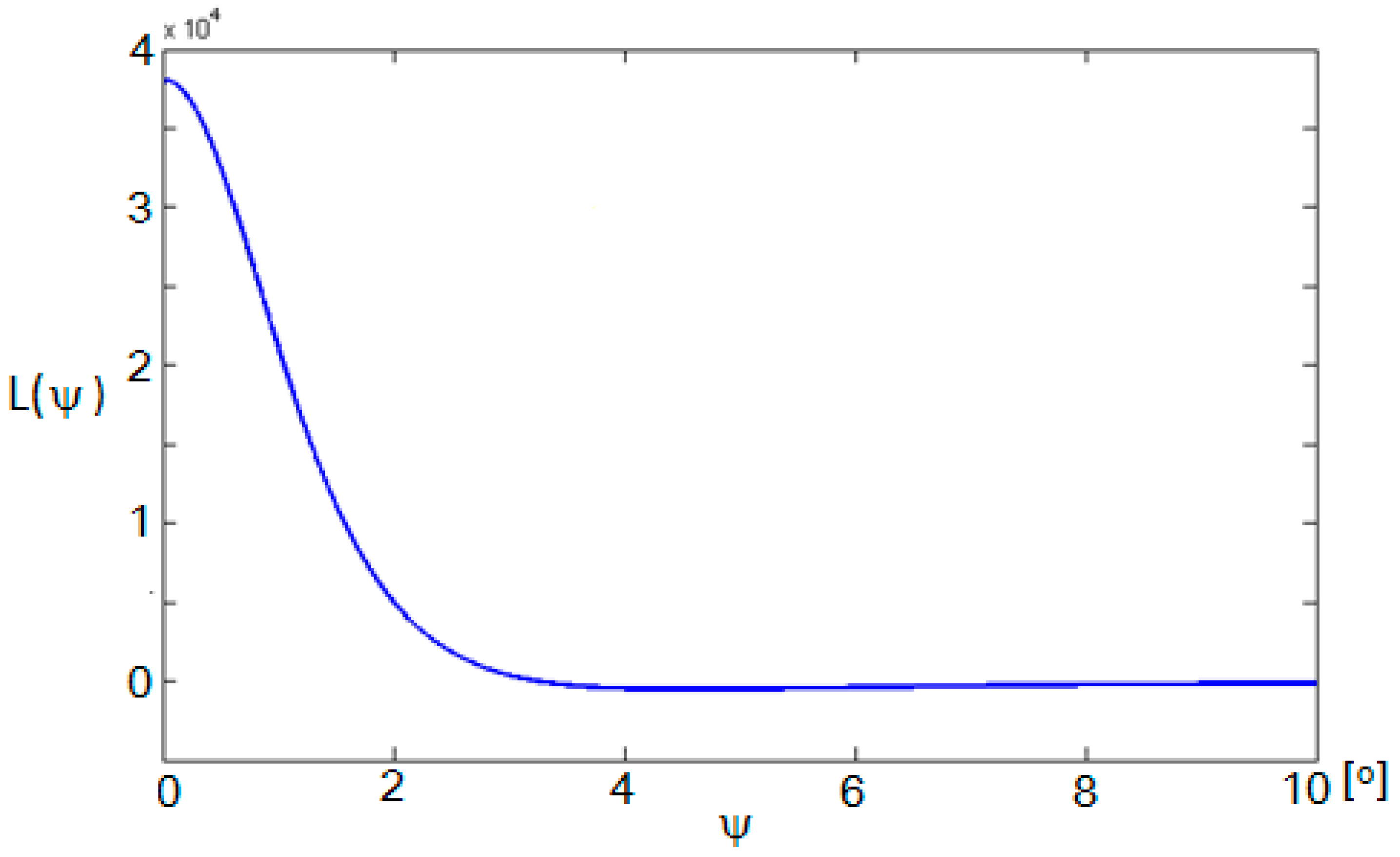
2.4. Kernel Behavior
To compute the parameter
W, the integral equation in Equation (16) is discretized and then solved numerically. The dependence of result on the integration domain can be investigated from a spatial behavior of the integral kernel
L. The gravity inversion could be localized if the integral kernel attenuates quickly with an increasing spherical distance [
34,
35]. The inversion is then carried out using only data within the near zone, while the far-zone contribution is disregarded. The near zone is chosen so that truncation errors due to disregarding the far-zone contribution are negligible.
A spatial behavior of the integral kernel
L is illustrated in
Figure 1. The kernel attenuates very quickly already at 2 arc-deg of the spherical distance with nearly zero values at 4 arc-deg. The near-zone limit
ψ ≤ 4 arc-deg thus sufficiently reduces truncation errors.
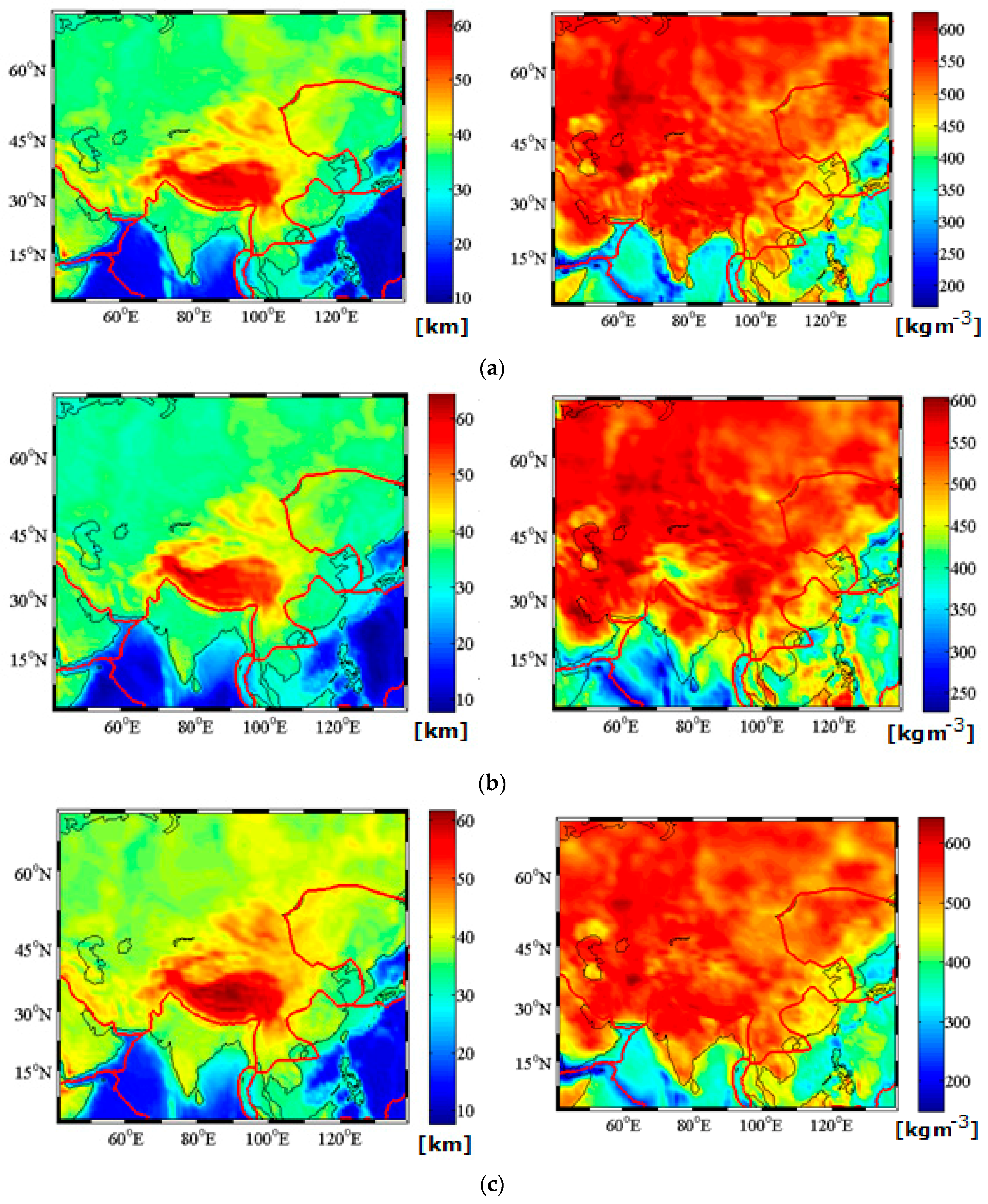
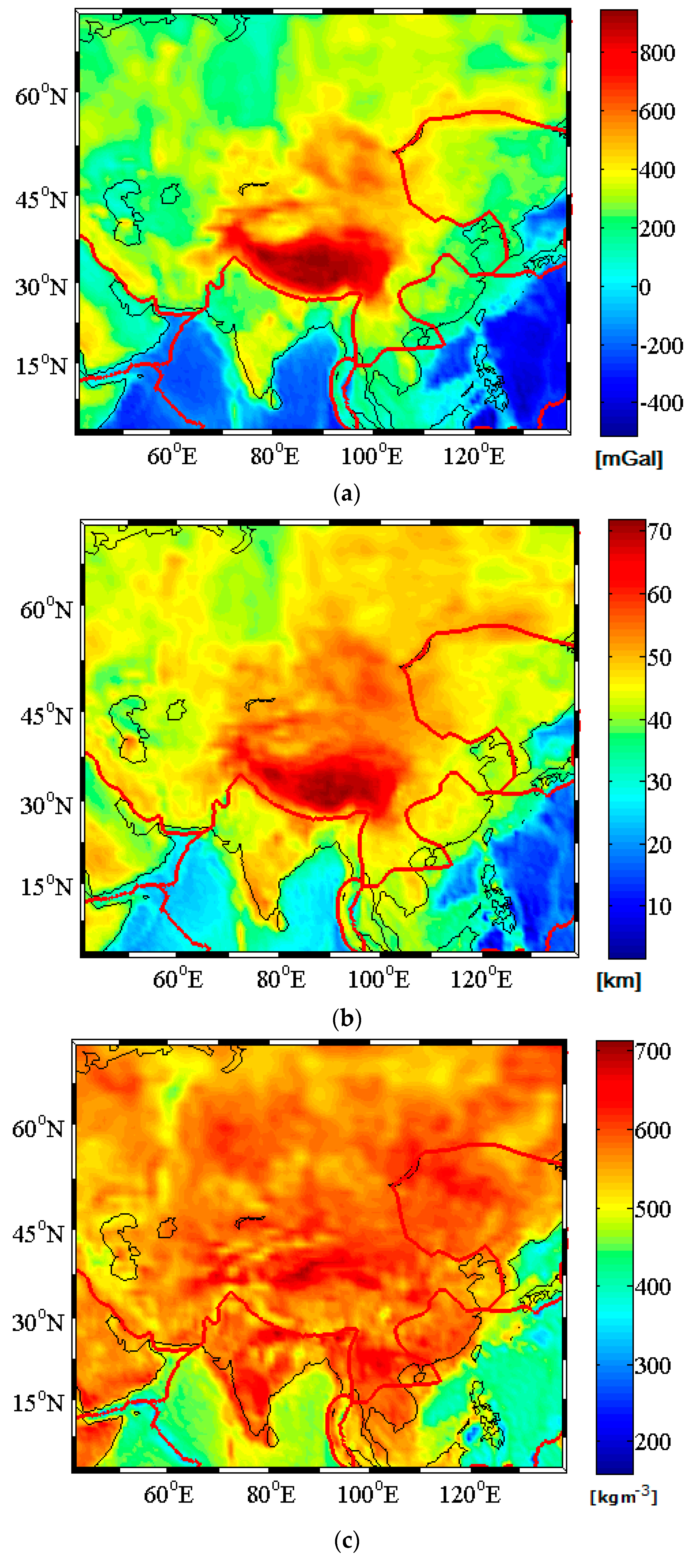
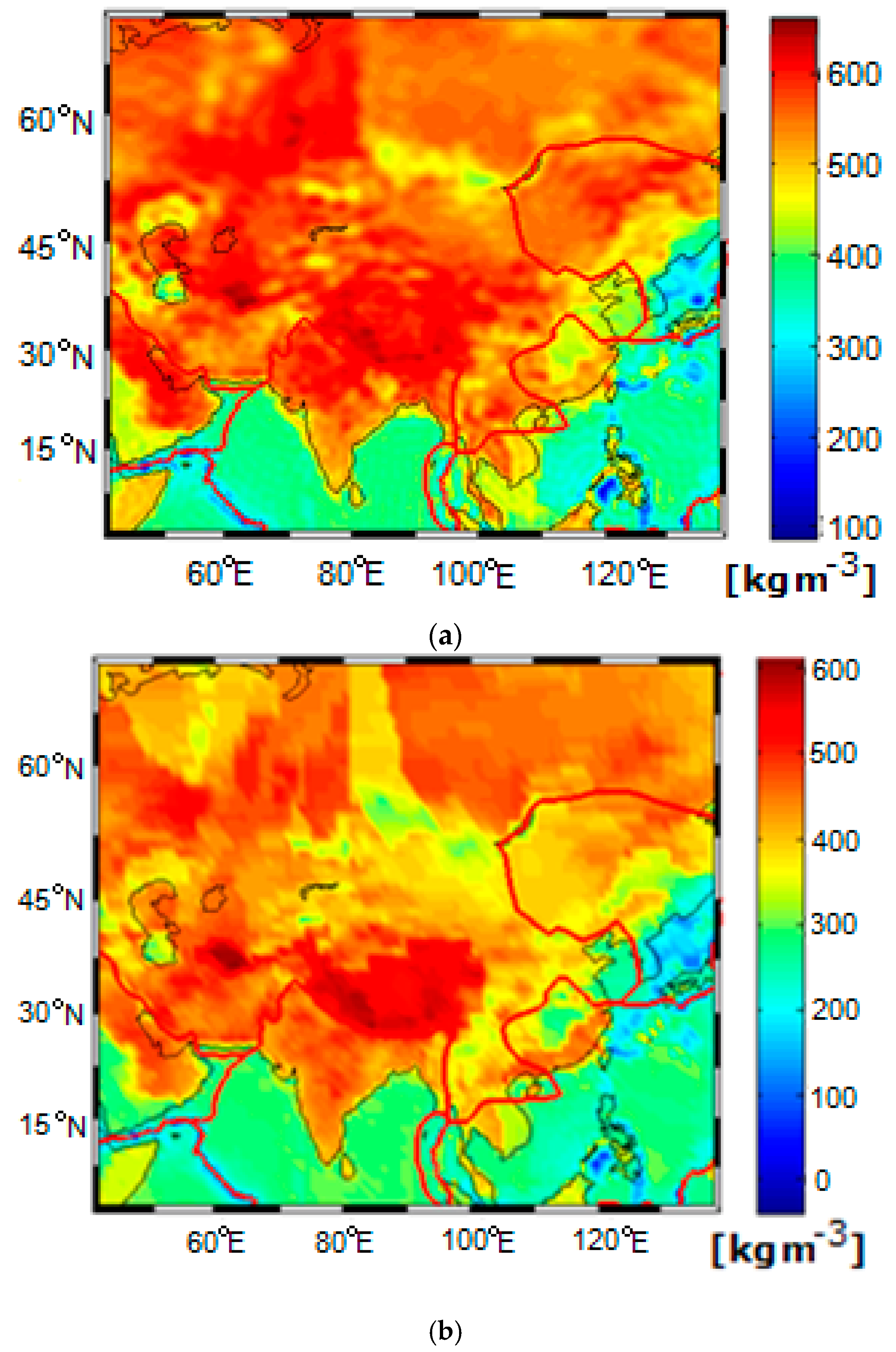
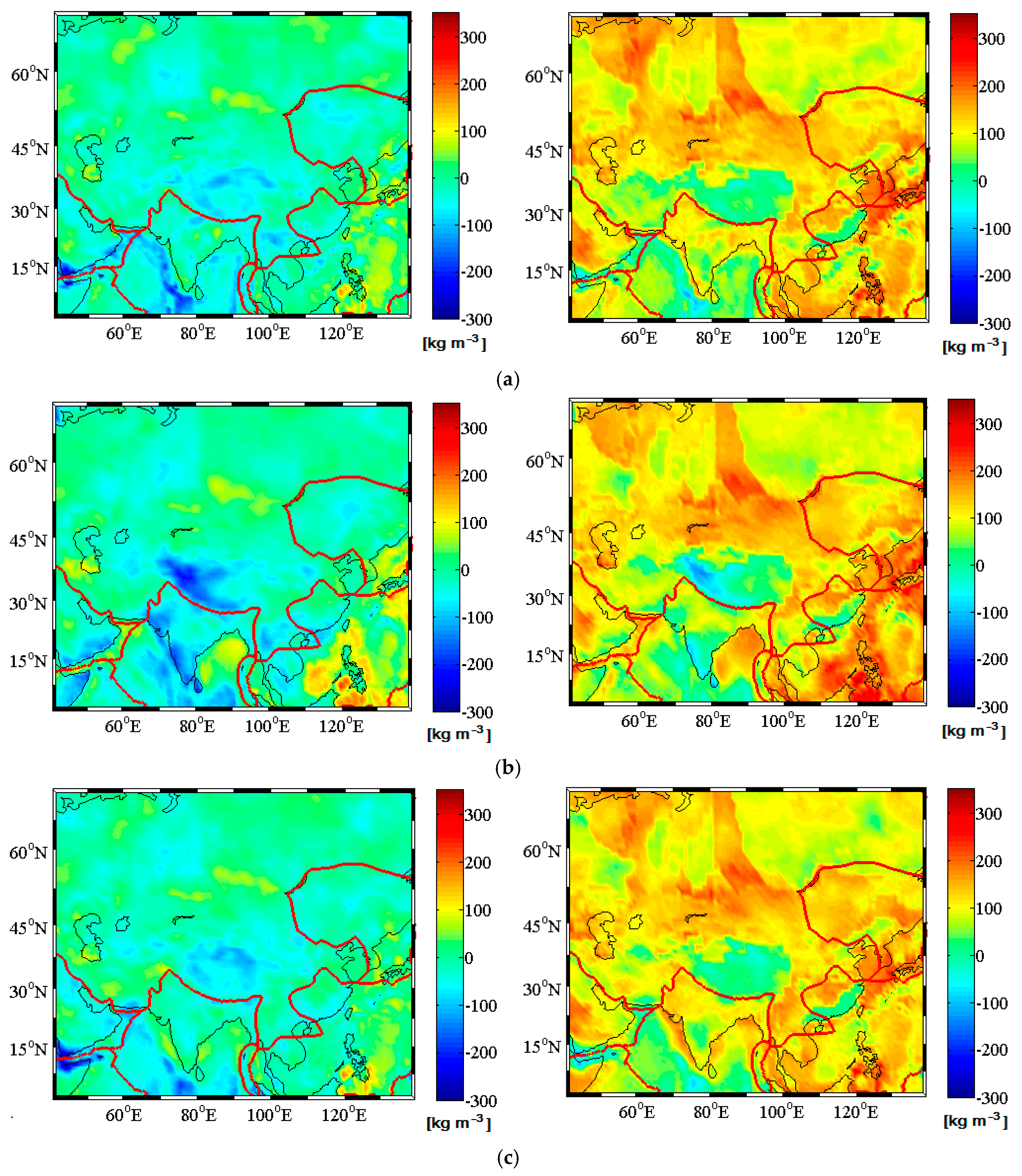
4. Summary and Concluding Remarks
We have developed the combined method for a determination of the Moho parameters from the GOCE in-orbit gravity gradients and constrained using seismic crustal model. We applied this method to investigate the Moho density contrast under most of Eurasia including surrounding continental and oceanic areas. The input data used for computation involved the topographic information from the SRTM on land, the bathymetric information derived from processing the satellite-altimetry data offshore, the sediment density and thickness information from the CRUST1.0 data and the vertical gravity gradients obtained from processing the GOCE satellite observables. The least-squares technique, applied for a regional Moho recovery, was formulated for the system of condition equations and solved based on finding the minimum-norm solution in order to obtain an optimal fit between gravimetric and seismic models. The condition equations were defined for mean values of seismic Moho parameters in order to suppress errors from areas with insufficient seismic-data coverage.
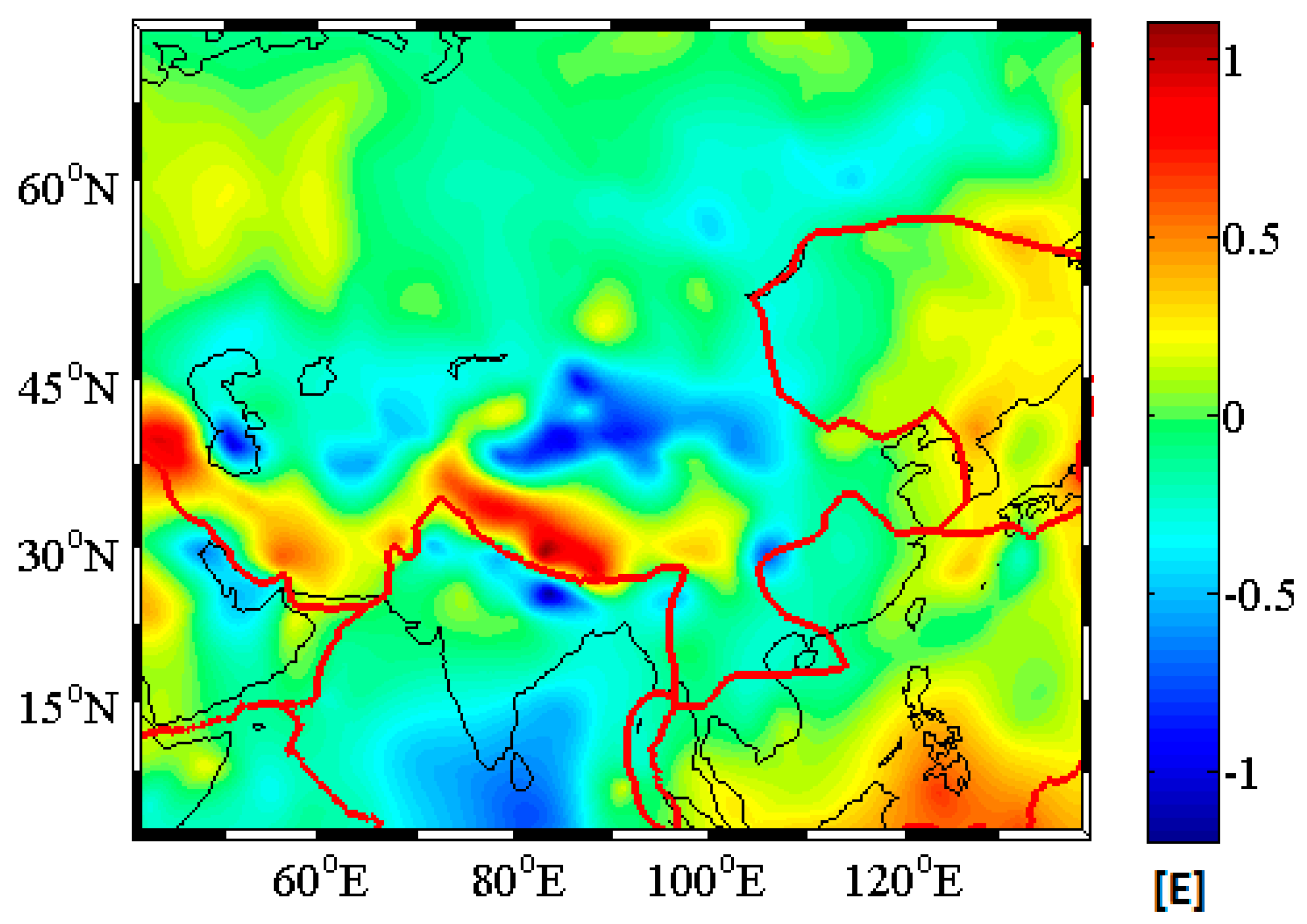
Our results confirmed large variations of the Moho density contrast with minima along the mid-oceanic rift zones and maxima under most of continental crustal structures. These results have a relatively good agreement with the CRUST1.0 and KTH1.0 models, but differ substantially from some previously published results of gravimetric studies. The most significant inconsistency was found in overestimated values of the Moho density contrast under Tibet and Himalaya, which according to [
23,
30] could reach 800 kg·m
−3 or even more. In more recent study [
43], however, much smaller values of the Moho density contrast were estimated (
i.e., the KTH1.0 model). Moreover, the Moho density contrast according to [
46] could hardly exceed 600 kg·m
−3 and much smaller values of the Moho density contrast were also reported in various seismic studies. In this study, we have confirmed these findings by showing that the Moho density contrast under most of the Eurasian continental crust is typically very uniform with most of the values being within a range from 400 to 600 kg·m
−3.


