
Evaluation of MODIS Gross Primary Production across Multiple Biomes in China Using Eddy Covariance Flux Data


Abstract
:
1. Introduction
2. Materials and Methods
2.1. Materials
2.1.1. MODIS GPP Algorithm
2.1.2. Meteorological Data
- NCEP-DOE Reanalysis II Data
- Site Meteorological Data
2.1.3. GLASS LAI Data
2.1.4. EC Flux Data
2.2. Methods
2.2.1. Experimental Design
2.2.2. Analytical Methods
3. Results
3.1. GPP Validation
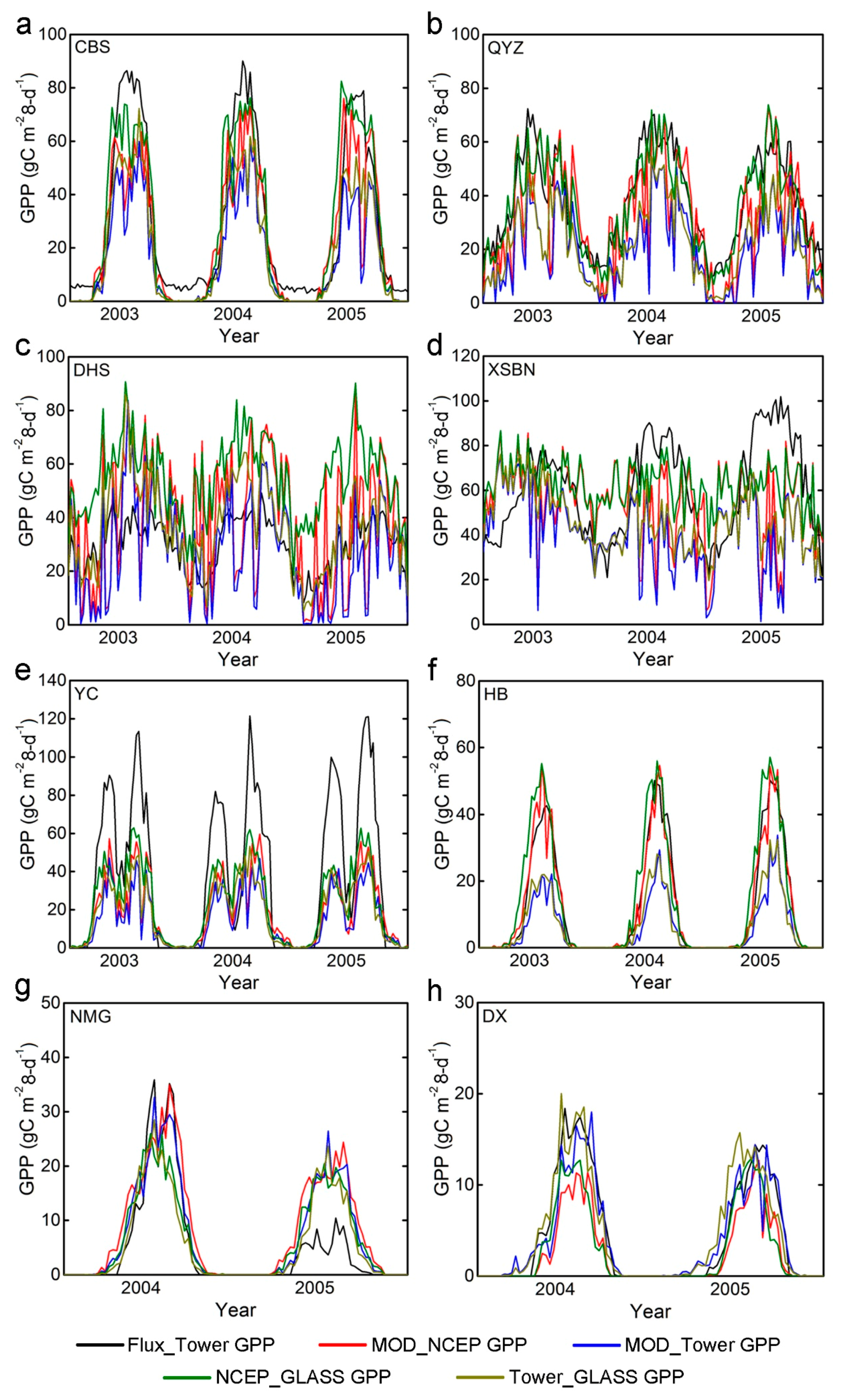
3.1.1. Eight-Day GPP
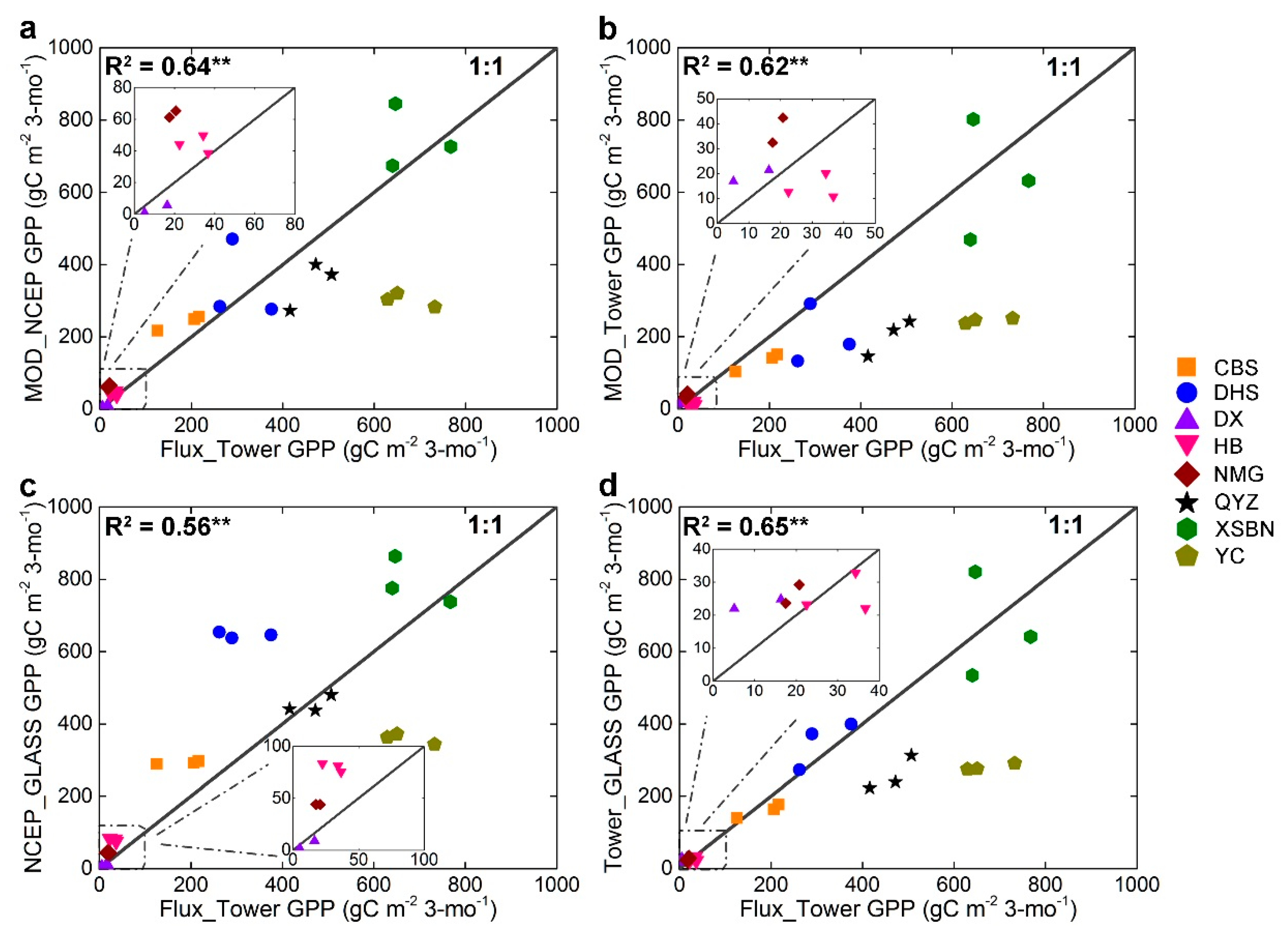
3.1.2. Seasonal GPP
- (1)
- Spring (March–May): The estimation performances of MOD_NCEP GPP (R2 = 0.64) and Tower_GLASS GPP (R2 = 0.65) were excellent (Figure 4, Table 3). The MOD_NCEP GPP, MOD_Tower GPP and Tower_GLASS GPP underestimated the Flux_Tower GPP to varying degrees (−39 gC·m−2·3-month−1, −122 gC·m−2·3-month−1 and −80 gC·m−2·3-month−1, respectively), primarily because of the considerable underestimation for QYZ and YC (Figure 4a,b,d). In contrast, NCEP_GLASS GPP overestimated the Flux_Tower GPP (40 gC·m−2·3-month−1) because the measurements for DHS were considerably overestimated (Figure 4c).
- (2)
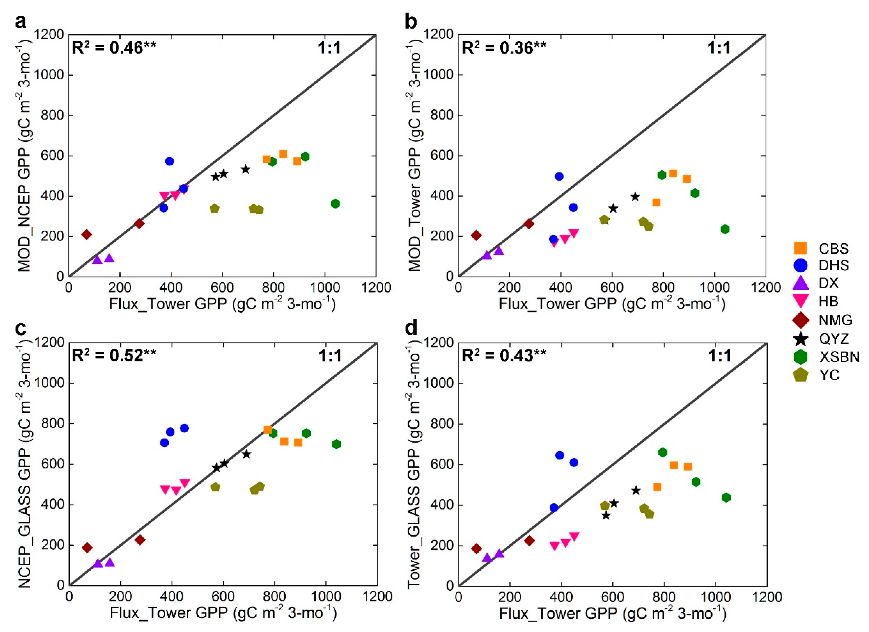
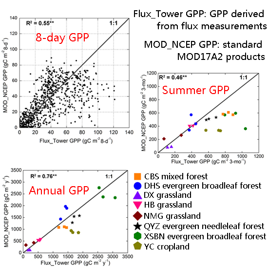
- Summer (June–August): None of the four algorithms estimated the Flux_Tower GPP effectively (Figure 5, Table 3). The main reason that the Flux_Tower GPP were seriously underestimated by the MOD_NCEP GPP, MOD_Tower GPP and Tower_GLASS GPP algorithms (−143 gC·m−2·3-month−1, −254 gC·m−2·3-month−1 and −161 gC·m−2·3-month−1, respectively) was that the measurements for CBS, QYZ, XSBN and YC were considerably underestimated (Figure 5a,b,d).
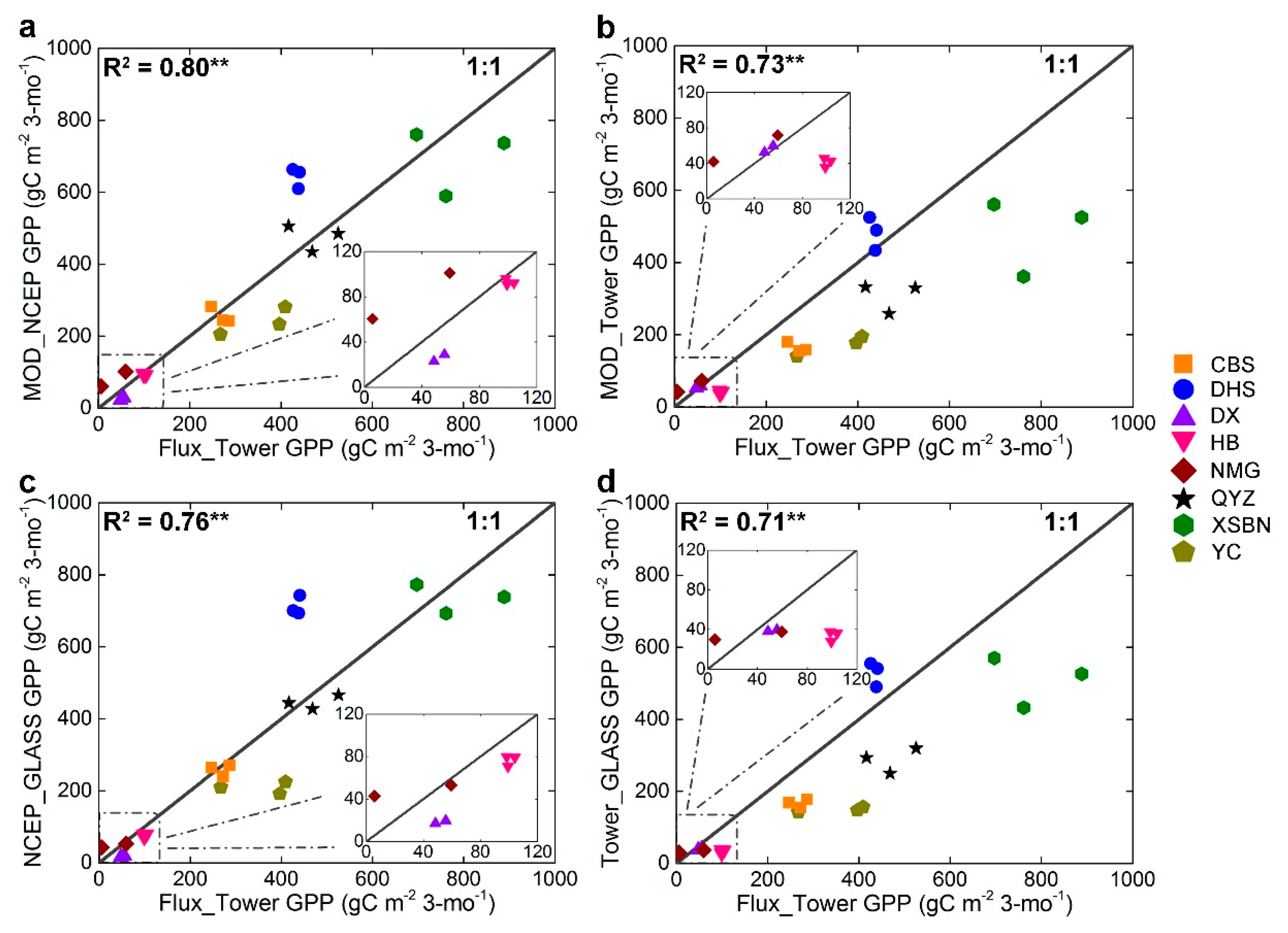
- (3)
- Autumn (September–November): The MOD_NCEP GPP (R2 = 0.80, Bias = 0 gC·m−2·3-month−1 and RMSE = 32%) and NCEP_GLASS GPP (R2 = 0.76, Bias = 1 gC·m−2·3-month−1 and RE = 57%) provided better estimating effectiveness (Figure 6, Table 3). In contrast, the MOD_Tower GPP and Tower_GLASS GPP obviously underestimated the Flux_Tower GPP (−102 gC·m−2·3-month−1) as a result of the common underestimations for CBS, HB, QYZ, XSBN and YC (Figure 6b,d).
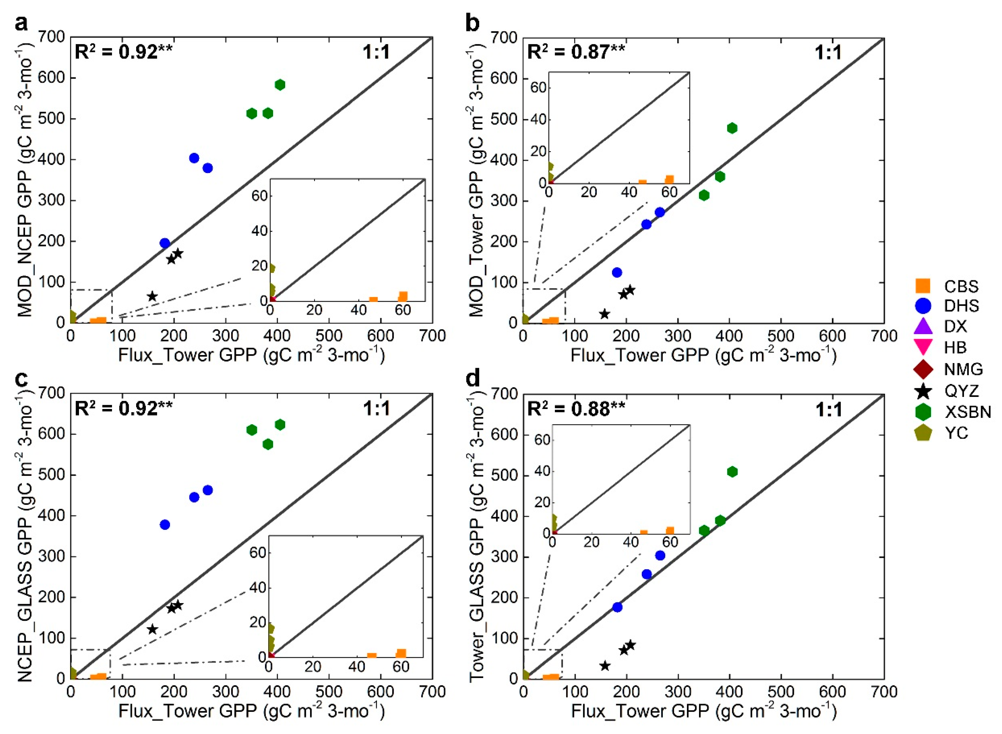
- (4)
- Winter (January–February and December): All four algorithms effectively estimated the Flux_Tower GPP (Figure 7, Table 3). However, the MOD_NCEP GPP and NCEP_GLASS GPP algorithms seriously overestimated the Flux_Tower GPP for DHS and XSBN (Figure 7a,c). The Flux_Tower GPP for QYZ were severely underestimated by the MOD_Tower GPP and Tower_GLASS GPP algorithms (Figure 7b,d).
3.1.3. Annual GPP
3.2. Meteorology
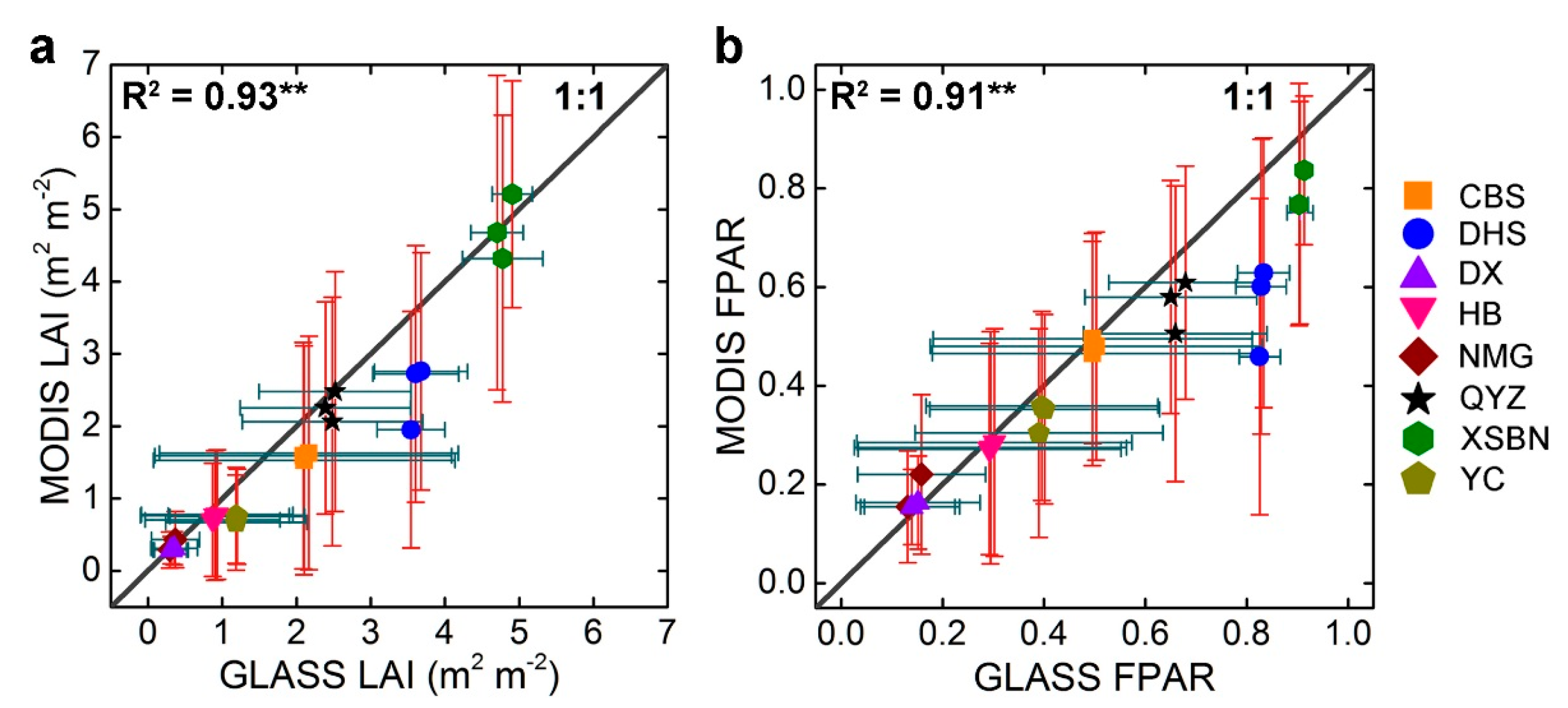
3.3. LAI and FPAR
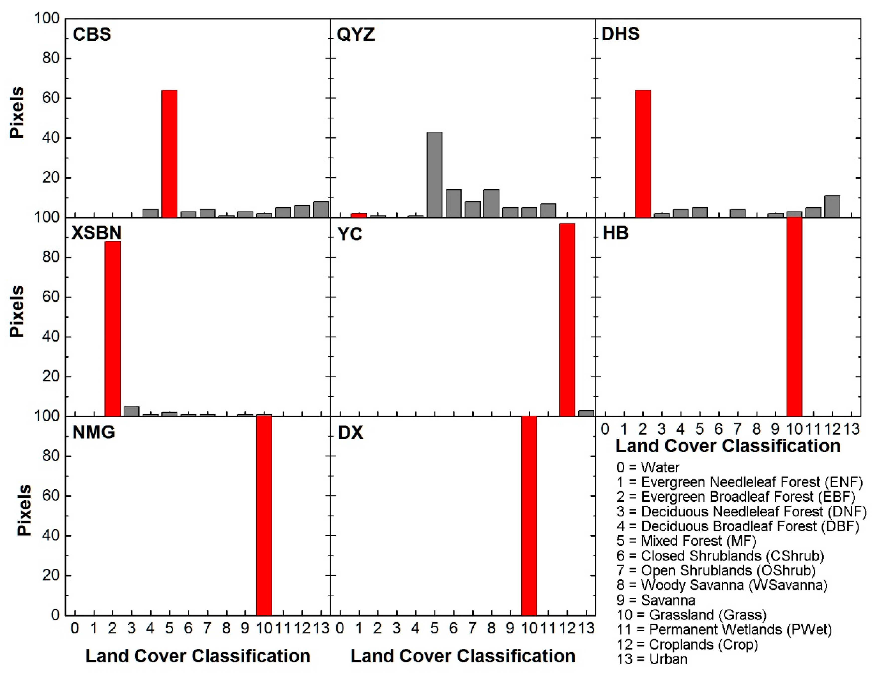
3.4. Land Cover
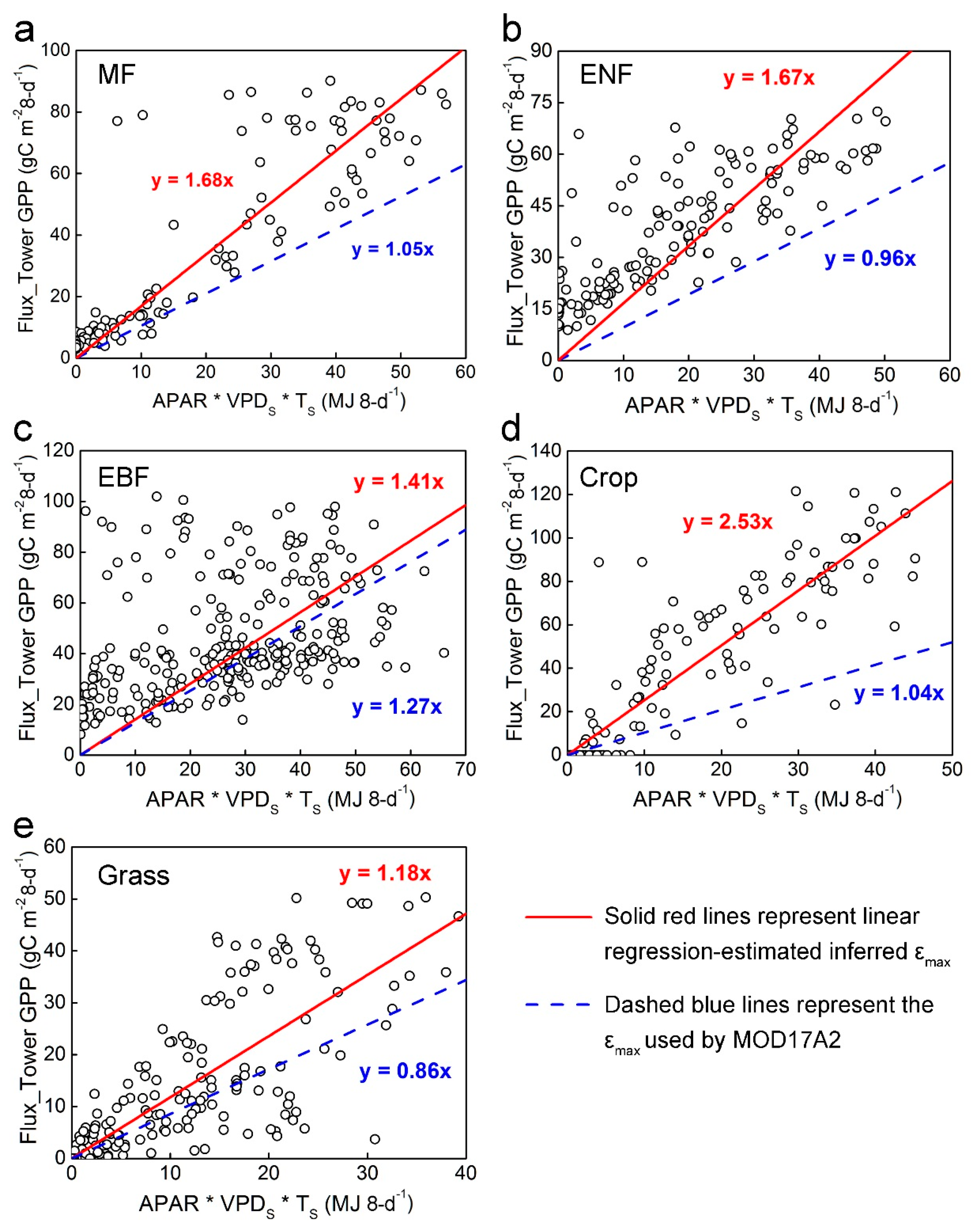
3.5. Light Use Efficiency
4. Discussion
4.1. Impact of Meteorology on MODIS GPP
4.2. Impact of LAI/FPAR on MODIS GPP
4.3. Impact of Land Cover on MODIS GPP
4.4. Impact of LUE on MODIS GPP
4.5. Uncertainties, Errors, and Accuracies
5. Conclusions
- (1)
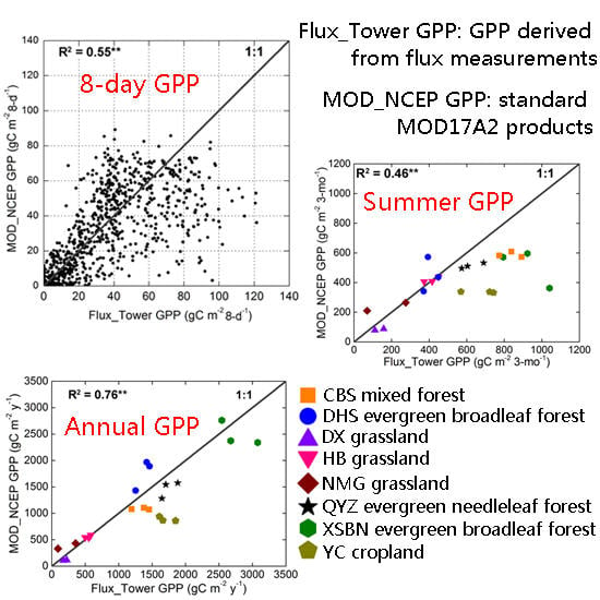
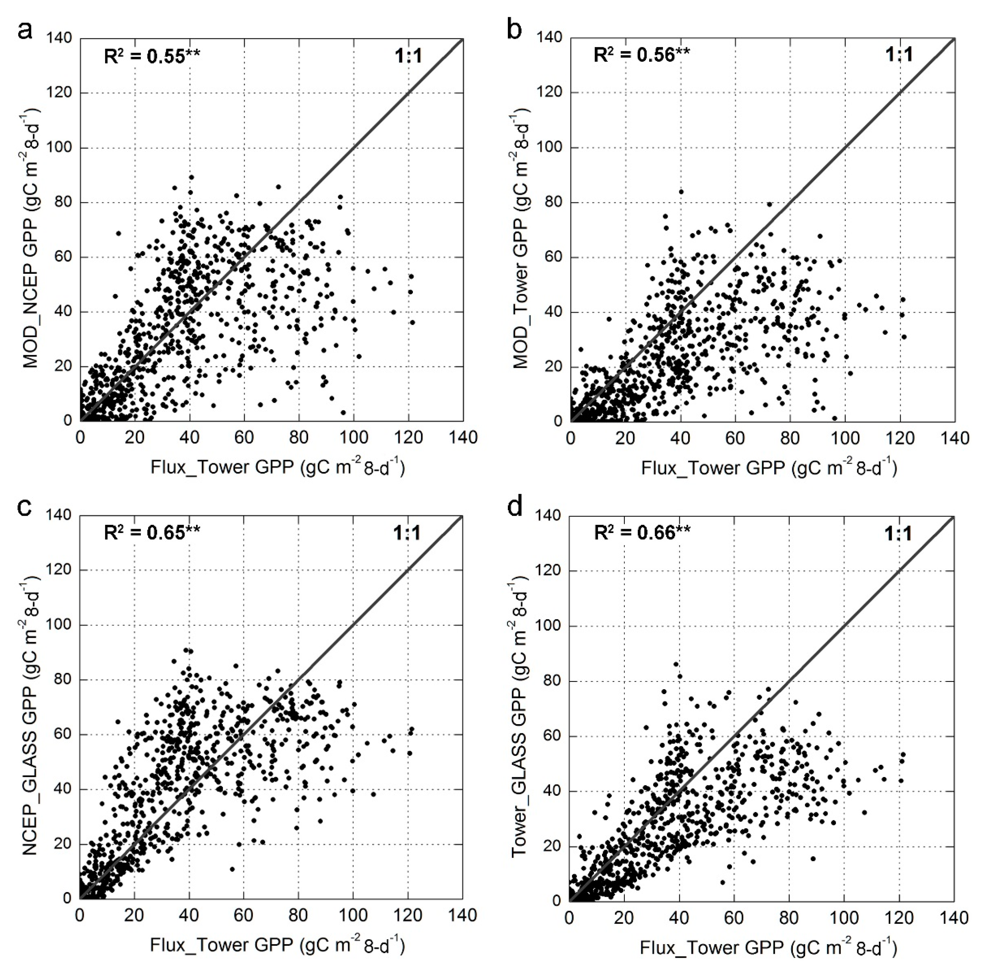
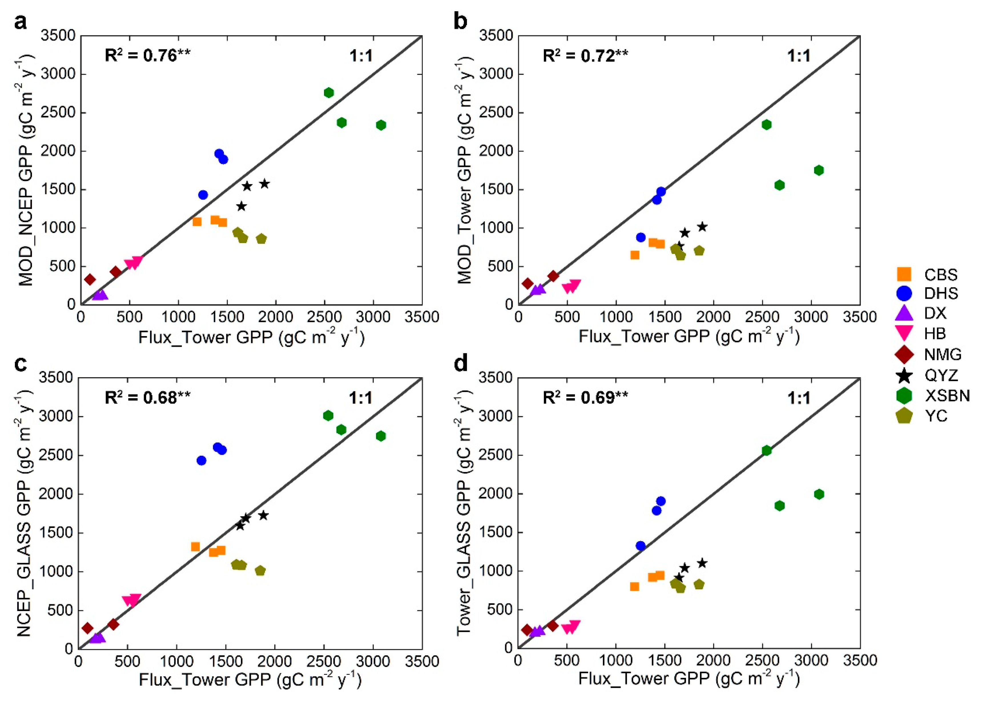
- The standard MOD17A2 product (i.e., MOD_NCEP GPP) performed better at estimating the annual GPP (R2 = 0.76) and agreed well with the tower GPP during the autumn (R2 = 0.80) and winter (R2 = 0.92). However, the effectiveness of the MOD_NCEP GPP algorithm for estimating GPP over eight days was poor (R2 = 0.55) and even worse during the summer (R2 = 0.46). In addition, the MOD_NCEP GPP algorithm was ineffective when estimating the annual GPP for mixed forests, evergreen needleleaf forests and cropland.
- (2)
- Replacing the NCEP-DOE Reanalysis II meteorology data with the site meteorology data (i.e., MOD_Tower GPP) only slightly improved the correlation with the tower GPP over eight days (R2 = 0.56). However, substantial improvements in estimating the tower GPP over eight days (R2 = 0.65) and during the summer (R2 = 0.52) were achieved by substituting GLASS_FPAR for MODIS_FPAR (i.e., NCEP_GLASS GPP). For cropland, the GPP estimates were more accurate after the FPAR data were improved. When the meteorology inputs and FPAR data were simultaneously replaced with improved data (i.e., Tower_GLASS GPP), the effectiveness in estimating the tower GPP was improved significantly for mixed forests and evergreen needleleaf forests.
- (3)
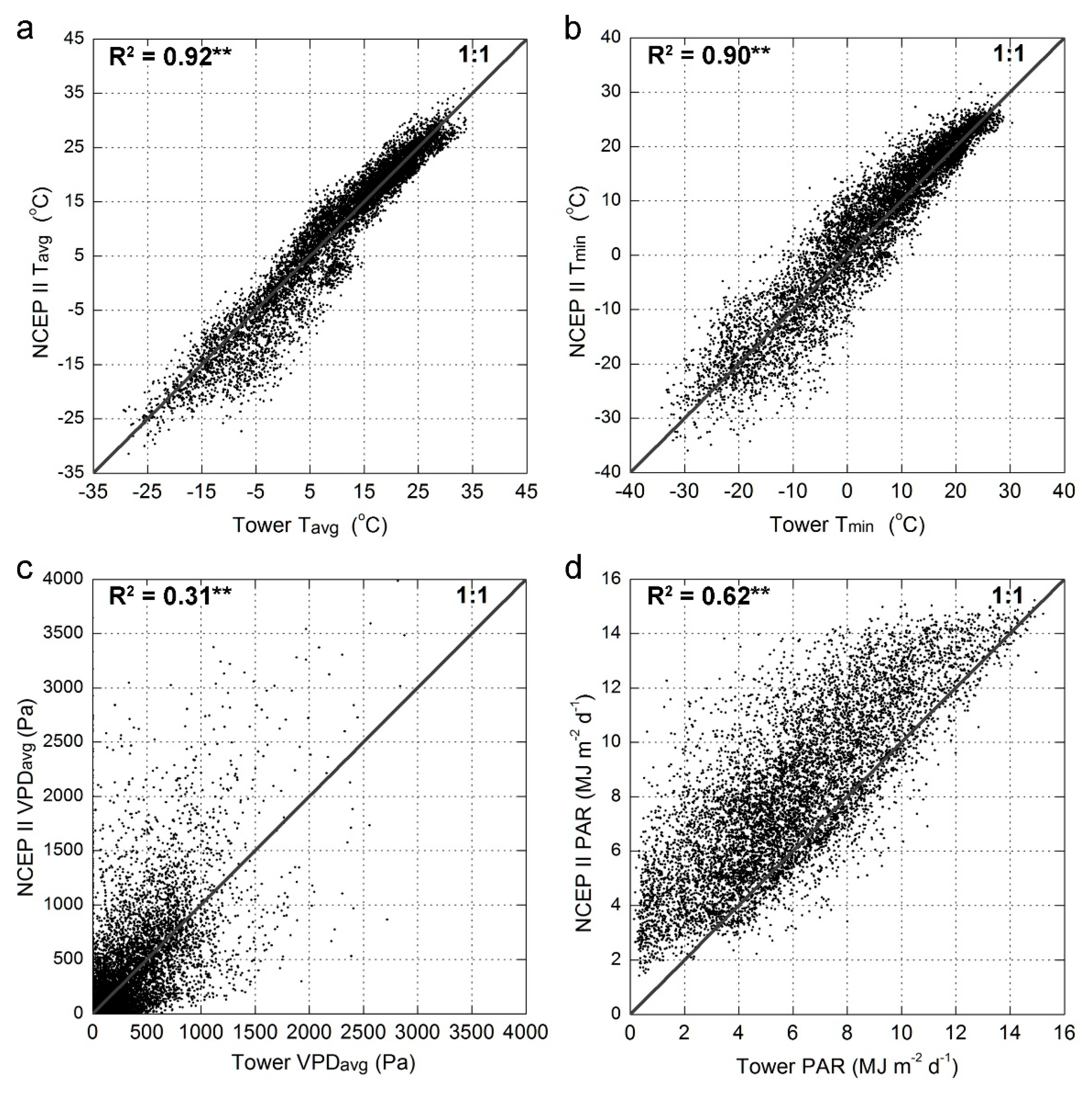
- There are four potential error sources related to the inputs of the MOD17A2 algorithm: meteorology, LAI/FPAR, land cover and εmax. The NCEP-DOE Reanalysis II meteorology data failed in estimating the tower measured VPD (R2 = 0.31), and MODIS_FPAR underestimated the improved FPAR data at most sites. Although MCD12Q1 succeeded in classifying most of the sites correctly, the values of MOD17A2 εmax were much smaller than the optimized εmax values for all five biome types discussed in this paper.
Acknowledgments
Author Contributions
Conflicts of Interest
References
- Gebremichael, M.; Barros, A. Evaluation of MODIS Gross Primary Productivity (GPP) in tropical monsoon regions. Remote Sens. Environ. 2006, 100, 150–166. [Google Scholar] [CrossRef]
- Beer, C.; Reichstein, M.; Tomelleri, E.; Ciais, P.; Jung, M.; Carvalhais, N.; Rodenbeck, C.; Arain, M.A.; Baldocchi, D.; Bonan, G.B.; et al. Terrestrial gross carbon dioxide uptake: Global distribution and covariation with climate. Science 2010, 329, 834–838. [Google Scholar] [CrossRef] [PubMed]
- Kotchenova, S.Y.; Song, X.; Shabanov, N.V.; Potter, C.S.; Knyazikhin, Y.; Myneni, R.B. Lidar remote sensing for modeling gross primary production of deciduous forests. Remote Sens. Environ. 2004, 92, 158–172. [Google Scholar] [CrossRef]
- Gitelson, A.A.; Viña, A.; Verma, S.B.; Rundquist, D.C.; Arkebauer, T.J.; Keydan, G.; Leavitt, B.; Ciganda, V.; Burba, G.G.; Suyker, A.E. Relationship between gross primary production and chlorophyll content in crops: Implications for the synoptic monitoring of vegetation productivity. J. Geophys. Res. 2006, 111. [Google Scholar] [CrossRef]
- Yuan, W.; Liu, S.; Zhou, G.; Zhou, G.; Tieszen, L.L.; Baldocchi, D.; Bernhofer, C.; Gholz, H.; Goldstein, A.H.; Goulden, M.L.; et al. Deriving a light use efficiency model from eddy covariance flux data for predicting daily gross primary production across biomes. Agric. For. Meteorol. 2007, 143, 189–207. [Google Scholar] [CrossRef]
- Sims, D.; Rahman, A.; Cordova, V.; Elmasri, B.; Baldocchi, D.; Bolstad, P.; Flanagan, L.; Goldstein, A.; Hollinger, D.; Misson, L. A new model of gross primary productivity for North American ecosystems based solely on the enhanced vegetation index and land surface temperature from MODIS. Remote Sens. Environ. 2008, 112, 1633–1646. [Google Scholar] [CrossRef]
- Yang, Y.; Shang, S.; Guan, H.; Jiang, L. A novel algorithm to assess gross primary production for terrestrial ecosystems from MODIS imagery. J. Geophys. Res. 2013, 118, 590–605. [Google Scholar] [CrossRef]
- Rahman, A.F. Potential of MODIS EVI and surface temperature for directly estimating per-pixel ecosystem C fluxes. Geophys. Res. Lett. 2005, 32. [Google Scholar] [CrossRef]
- Wu, C.; Chen, J.M.; Huang, N. Predicting gross primary production from the enhanced vegetation index and photosynthetically active radiation: Evaluation and calibration. Remote Sens. Environ. 2011, 115, 3424–3435. [Google Scholar] [CrossRef]
- Lin, A.; Zhu, H.; Wang, L.; Gong, W.; Zou, L. Characteristics of long-term climate change and the ecological responses in central China. Earth Interact. 2016, 20, 1–24. [Google Scholar] [CrossRef]
- Zhao, M.; Heinsch, F.A.; Nemani, R.R.; Running, S.W. Improvements of the MODIS terrestrial gross and net primary production global data set. Remote Sens. Environ. 2005, 95, 164–176. [Google Scholar] [CrossRef]
- Kanniah, K.D.; Beringer, J.; Hutley, L.B.; Tapper, N.J.; Zhu, X. Evaluation of Collections 4 and 5 of the MODIS Gross Primary Productivity product and algorithm improvement at a tropical savanna site in northern Australia. Remote Sens. Environ. 2009, 113, 1808–1822. [Google Scholar] [CrossRef]
- Garbulsky, M.F.; Peñuelas, J.; Papale, D.; Ardö, J.; Goulden, M.L.; Kiely, G.; Richardson, A.D.; Rotenberg, E.; Veenendaal, E.M.; Filella, I. Patterns and controls of the variability of radiation use efficiency and primary productivity across terrestrial ecosystems. Glob. Ecol. Biogeogr. 2010, 19, 253–267. [Google Scholar] [CrossRef]
- Heinsch, F.A.; Zhao, M.; Running, S.W.; Kimball, J.S.; Nemani, R.R.; Davis, K.J.; Bolstad, P.V.; Cook, B.D.; Desai, A.R.; Ricciuto, D.M.; et al. Evaluation of remote sensing based terrestrial productivity from MODIS using regional tower eddy flux network observations. IEEE Tran. Geosci. Remote Sens. 2006, 7, 1908–1925. [Google Scholar] [CrossRef]
- Propastin, P.; Ibrom, A.; Knohl, A.; Erasmi, S. Effects of canopy photosynthesis saturation on the estimation of gross primary productivity from MODIS data in a tropical forest. Remote Sens. Environ. 2012, 121, 252–260. [Google Scholar] [CrossRef]
- Coops, N.; Black, T.; Jassal, R.; Trofymow, J.; Morgenstern, K. Comparison of MODIS, eddy covariance determined and physiologically modelled gross primary production (GPP) in a Douglas-fir forest stand. Remote Sens. Environ. 2007, 107, 385–401. [Google Scholar] [CrossRef]
- Groenendijk, M.; Dolman, A.J.; van der Molen, M.K.; Leuning, R.; Arneth, A.; Delpierre, N.; Gash, J.H.C.; Lindroth, A.; Richardson, A.D.; Verbeeck, H.; et al. Assessing parameter variability in a photosynthesis model within and between plant functional types using global Fluxnet eddy covariance data. Agric. For. Meteorol. 2011, 151, 22–38. [Google Scholar] [CrossRef]
- Wu, C.; Munger, J.W.; Niu, Z.; Kuang, D. Comparison of multiple models for estimating gross primary production using MODIS and eddy covariance data in Harvard Forest. Remote Sens. Environ. 2010, 114, 2925–2939. [Google Scholar] [CrossRef]
- Xiao, J.; Zhuang, Q.; Law, B.E.; Chen, J.; Baldocchi, D.D.; Cook, D.R.; Oren, R.; Richardson, A.D.; Wharton, S.; Ma, S. A continuous measure of gross primary production for the conterminous United States derived from MODIS and AmeriFlux data. Remote Sens. Environ. 2010, 114, 576–591. [Google Scholar] [CrossRef]
- Turner, D.P.; Ritts, W.D.; Cohen, W.B.; Gower, S.T.; Zhao, M.; Running, S.W.; Wofsy, S.C.; Urbanski, S.; Dunn, A.L.; Munger, J.W. Scaling Gross Primary Production (GPP) over boreal and deciduous forest landscapes in support of MODIS GPP product validation. Remote Sens. Environ. 2003, 88, 256–270. [Google Scholar] [CrossRef]
- Sjöström, M.; Zhao, M.; Archibald, S.; Arneth, A.; Cappelaere, B.; Falk, U.; de Grandcourt, A.; Hanan, N.; Kergoat, L.; Kutsch, W.; et al. Evaluation of MODIS gross primary productivity for Africa using eddy covariance data. Remote Sens. Environ. 2013, 131, 275–286. [Google Scholar] [CrossRef]
- Wang, X.; Ma, M.; Li, X.; Song, Y.; Tan, J.; Huang, G.; Zhang, Z.; Zhao, T.; Feng, J.; Ma, Z.; et al. Validation of MODIS-GPP product at 10 flux sites in northern China. Int. J. Remote Sens. 2013, 34, 587–599. [Google Scholar] [CrossRef]
- John, R.; Chen, J.; Noormets, A.; Xiao, X.; Xu, J.; Lu, N.; Chen, S. Modelling gross primary production in semi-arid Inner Mongolia using MODIS imagery and eddy covariance data. Int. J. Remote Sens. 2013, 34, 2829–2857. [Google Scholar] [CrossRef]
- Zhang, Y.; Yu, Q.; Jiang, J.; Tang, Y. Calibration of Terra/MODIS gross primary production over an irrigated cropland on the North China Plain and an alpine meadow on the Tibetan Plateau. Glob. Chang. Biol. 2008, 14, 757–767. [Google Scholar] [CrossRef]
- Liu, Z.; Shao, Q.; Liu, J. The performances of MODIS-GPP and -ET products in China and their sensitivity to input data (FPAR/LAI). Remote Sens. 2015, 7, 135–152. [Google Scholar] [CrossRef]
- Guan, D.; Wu, J.; Zhao, X.; Han, S.; Yu, G.; Sun, X.; Jin, C. CO2 fluxes over an old, temperate mixed forest in northeastern China. Agric. For. Meteorol. 2006, 137, 138–149. [Google Scholar] [CrossRef]
- Wen, X.; Yu, G.; Sun, X.; Li, Q.; Liu, Y.; Zhang, L.; Ren, C.; Fu, Y.; Li, Z. Soil moisture effect on the temperature dependence of ecosystem respiration in a subtropical Pinus plantation of southeastern China. Agric. For. Meteorol. 2006, 137, 166–175. [Google Scholar] [CrossRef]
- Zhang, L.; Yu, G.; Sun, X.; Wen, X.; Ren, C.; Fu, Y.; Li, Q.; Li, Z.; Liu, Y.; Guan, D.; et al. Seasonal variations of ecosystem apparent quantum yield (α) and maximum photosynthesis rate (Pmax) of different forest ecosystems in China. Agric. For. Meteorol. 2006, 137, 176–187. [Google Scholar] [CrossRef]
- Yu, G.; Wen, X.; Sun, X.; Tanner, B.D.; Lee, X.; Chen, J. Overview of ChinaFLUX and evaluation of its eddy covariance measurement. Agric. For. Meteorol. 2006, 137, 125–137. [Google Scholar] [CrossRef]
- Sun, X.; Zhu, Z.; Wen, X.; Yuan, G.; Yu, G. The impact of averaging period on eddy fluxes observed at ChinaFLUX sites. Agric. For. Meteorol. 2006, 137, 188–193. [Google Scholar] [CrossRef]
- Fu, Y.; Yu, G.; Sun, X.; Li, Y.; Wen, X.; Zhang, L.; Li, Z.; Zhao, L.; Hao, Y. Depression of net ecosystem CO2 exchange in semi-arid Leymus chinensis steppe and alpine shrub. Agric. For. Meteorol. 2006, 137, 234–244. [Google Scholar] [CrossRef]
- Monteith, J.L. Solar radiation and production in tropical ecosystems. J. Appl. Ecol. 1972, 9, 747–766. [Google Scholar] [CrossRef]
- Running, S.W.; Thornton, P.E.; Nemani, R.R.; Glassy, J.M. Global terrestrial gross and net primary productivity from the Earth observing system. In Methods in Ecosystem Science; Sala, O., Jackson, R., Mooney, H., Eds.; Springer: New York, NY, USA, 2000; pp. 44–57. [Google Scholar]
- Heinsch, F.A.; Reeves, M.; Votava, P.; Kang, S.; Milesi, C.; Zhao, M.; Glassy, J.; Jolly, W.M.; Loehman, R.; Bowker, C.F.; et al. User’s Guide: GPP and NPP (MOD17A2/A3) Products NASA MODIS Land Algorithm; University of Montana: Missoula, MT, USA, 2003; p. 57. [Google Scholar]
- Zhao, M.; Running, S.W. Drought-induced reduction in global terrestrial net primary production from 2000 through 2009. Science 2010, 329, 940–943. [Google Scholar] [CrossRef] [PubMed]
- Level 1 and Atmosphere Archive and Distribution System (LAADS). Available online: https://ladsweb.nascom.nasa.gov/index.html (accessed on 3 May 2015).
- Friedl, M.A.; Sulla-Menashe, D.; Tan, B.; Schneider, A.; Ramankutty, N.; Sibley, A.; Huang, X. MODIS collection 5 global land cover: Algorithm refinements and characterization of new datasets. Remote Sens. Environ. 2010, 114, 168–182. [Google Scholar] [CrossRef]
- Earth System Research Laboratory. Available online: http://www.esrl.noaa.gov/psd/about/index.html (accessed on 11 May 2015).
- China Meteorological Administration. Available online: http://cdc.nmic.cn/home.do (accessed on 7 June 2014).
- Peng, Y.; Gitelson, A.A.; Sakamoto, T. Remote estimation of gross primary productivity in crops using MODIS 250 m data. Remote Sens. Environ. 2013, 128, 186–196. [Google Scholar] [CrossRef]
- Xiao, Z.; Liang, S.; Wang, J.; Chen, P.; Yin, X.; Zhang, L.; Song, J. Use of general regression neural networks for generating the GLASS leaf area index product from time-series MODIS surface reflectance. IEEE Trans. Geosci. Remote Sens. 2014, 52, 209–223. [Google Scholar] [CrossRef]
- Zhao, X.; Liang, S.; Liu, S.; Yuan, W.; Xiao, Z.; Liu, Q.; Cheng, J.; Zhang, X.; Tang, H.; Zhang, X.; et al. The Global Land Surface Satellite (GLASS) remote sensing data processing system and products. Remote Sens. 2013, 5, 2436–2450. [Google Scholar] [CrossRef]
- Liang, S.; Zhao, X.; Liu, S.; Yuan, W.; Cheng, X.; Xiao, Z.; Zhang, X.; Liu, Q.; Cheng, J.; Tang, H.; et al. A long-term Global LAnd Surface Satellite (GLASS) data-set for environmental studies. Int. J. Digit. Earth 2013, 6, 5–33. [Google Scholar] [CrossRef]
- Generation and Applications of Global Products of Essential Land Variables. Available online: http://glass-product.bnu.edu.cn (accessed on 21 July 2015).
- Turner, D.P.; Ritts, W.D.; Cohen, W.B.; Gower, S.T.; Running, S.W.; Zhao, M.; Costa, M.H.; Kirschbaum, A.A.; Ham, J.M.; Saleska, S.R.; et al. Evaluation of MODIS NPP and GPP products across multiple biomes. Remote Sens. Environ. 2006, 102, 282–292. [Google Scholar] [CrossRef]
- ChinaFLUX. Available online: http://www.chinaflux.org (accessed on 29 May 2015).
- Yu, G.; Zhu, X.; Fu, Y.; He, H.; Wang, Q.; Wen, X.; Li, X.; Zhang, L.; Zhang, L.; Su, W.; et al. Spatial patterns and climate drivers of carbon fluxes in terrestrial ecosystems of China. Glob. Chang. Biol. 2013, 19, 798–810. [Google Scholar] [CrossRef] [PubMed]
- He, M.; Zhou, Y.; Ju, W.; Chen, J.; Zhang, L.; Wang, S.; Saigusa, N.; Hirata, R.; Murayama, S.; Liu, Y. Evaluation and improvement of MODIS gross primary productivity in typical forest ecosystems of East Asia based on eddy covariance measurements. J. For. Res. 2013, 18, 31–40. [Google Scholar] [CrossRef]
- Chen, J.; Zhang, H.; Liu, Z.; Che, M.; Chen, B. Evaluating parameter adjustment in the MODIS gross primary production algorithm based on eddy covariance tower measurements. Remote Sens. 2014, 6, 3321–3348. [Google Scholar] [CrossRef]
- Zhao, M.; Running, S.W.; Nemani, R.R. Sensitivity of Moderate Resolution Imaging Spectroradiometer (MODIS) terrestrial primary production to the accuracy of meteorological reanalyses. J. Geophys. Res. 2006, 111. [Google Scholar] [CrossRef]
- Mu, Q.; Zhao, M.; Heinsch, F.A.; Liu, M.; Tian, H.; Running, S.W. Evaluating water stress controls on primary production in biogeochemical and remote sensing based models. J. Geophys. Res. 2007, 112. [Google Scholar] [CrossRef]
- Liu, Z.; Wang, L.; Wang, S. Comparison of different GPP models in China using MODIS image and ChinaFLUX data. Remote Sens. 2014, 6, 10215–10231. [Google Scholar] [CrossRef]
- Moffat, A.M.; Papale, D.; Reichstein, M.; Hollinger, D.Y.; Richardson, A.D.; Barr, A.G.; Beckstein, C.; Braswell, B.H.; Churkina, G.; Desai, A.R.; et al. Comprehensive comparison of gap-filling techniques for eddy covariance net carbon fluxes. Agric. For. Meteorol. 2007, 147, 209–232. [Google Scholar] [CrossRef]
- Nightingale, J.M.; Coops, N.C.; Waring, R.H.; Hargrove, W.W. Comparison of MODIS gross primary production estimates for forests across the U.S.A. with those generated by a simple process model, 3-PGS. Remote Sens. Environ. 2007, 109, 500–509. [Google Scholar] [CrossRef]
- He, M.; Ju, W.; Zhou, Y.; Chen, J.; He, H.; Wang, S.; Wang, H.; Guan, D.; Yan, J.; Li, Y.; et al. Development of a two-leaf light use efficiency model for improving the calculation of terrestrial gross primary productivity. Agric. For. Meteorol. 2013, 173, 28–39. [Google Scholar] [CrossRef]
- Hashimoto, H.; Wang, W.; Milesi, C.; Xiong, J.; Ganguly, S.; Zhu, Z.; Nemani, R. Structural uncertainty in model-simulated trends of global gross primary production. Remote Sens. 2013, 5, 1258–1273. [Google Scholar] [CrossRef]
- Zhang, F.; Chen, J.M.; Chen, J.; Gough, C.M.; Martin, T.A.; Dragoni, D. Evaluating spatial and temporal patterns of MODIS GPP over the conterminous U.S. against flux measurements and a process model. Remote Sens. Environ. 2012, 124, 717–729. [Google Scholar] [CrossRef]


| Sites (Abbreviation) | Lat (°N) | Lon (°E) | Biome Type | MAP (mm) | MAT (°C) | Data Range | References |
|---|---|---|---|---|---|---|---|
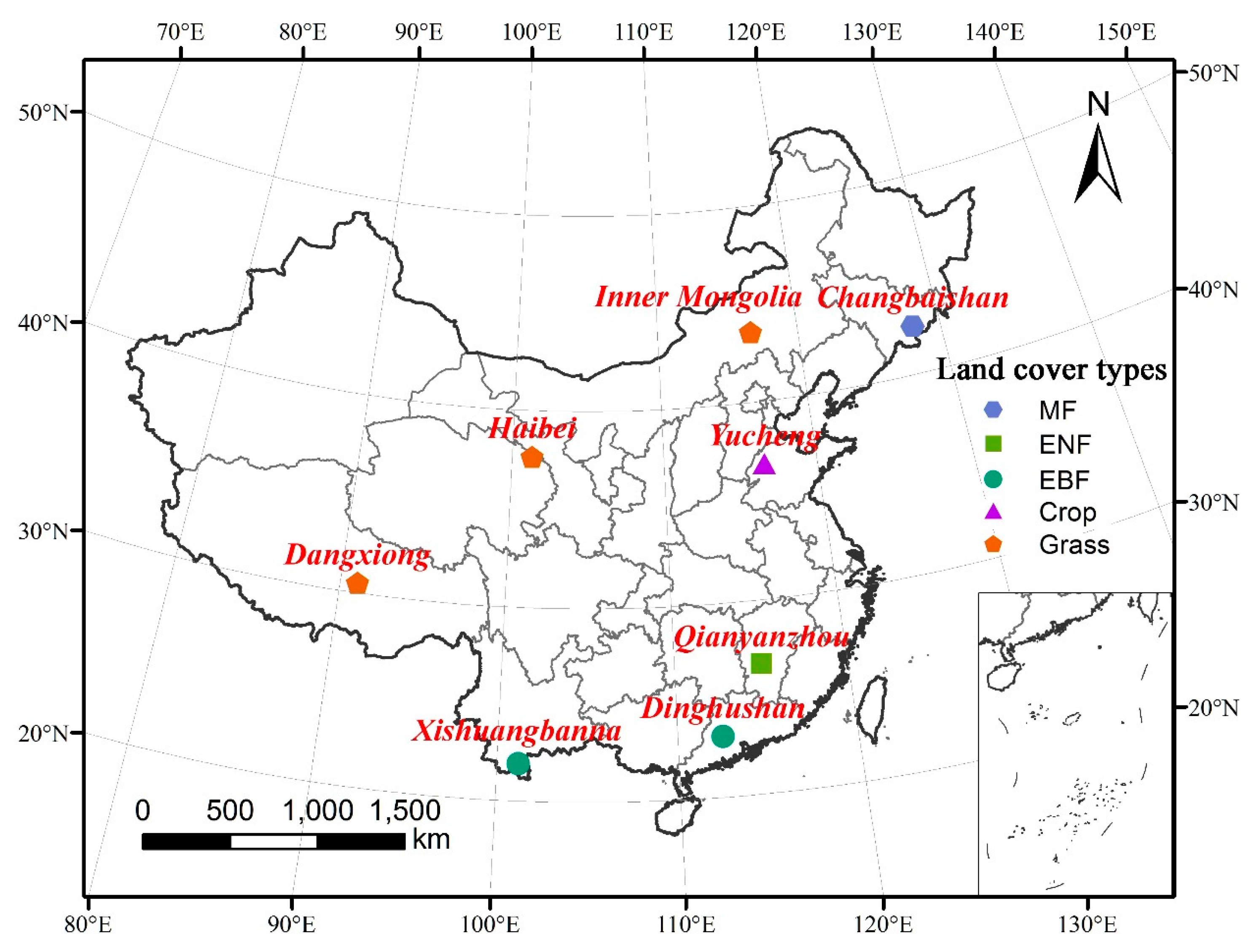
| Changbaishan forest site (CBS) | 42.40 | 128.10 | MF | 713 | 3.6 | 2003–2005 | Guan et al. (2006) [26] |
| Qianyanzhou forest site (QYZ) | 26.74 | 115.06 | ENF | 1542 | 17.9 | 2003–2005 | Wen et al. (2006) [27] |
| Dinghushan forest site (DHS) | 23.17 | 112.53 | EBF | 1956 | 20.9 | 2003–2005 | Zhang et al. (2006) [28] |
| Xishuangbanna forest site (XSBN) | 21.95 | 101.20 | EBF | 1493 | 21.8 | 2003–2005 | Yu et al. (2006) [29] |
| Yucheng cropland site (YC) | 36.83 | 116.57 | Crop | 582 | 13.1 | 2003–2005 | Sun et al. (2006) [30] |
| Haibei grassland site (HB) | 37.67 | 101.33 | Grass | 580 | −1.7 | 2003–2005 | Fu et al. (2006) [31] |
| Inner Mongolia grassland site (NMG) | 43.55 | 116.68 | Grass | 338 | 0.9 | 2004–2005 | Fu et al. (2006) [31] |
| Dangxiong grassland site (DX) | 30.50 | 91.07 | Grass | 450 | 1.3 | 2004–2005 | Yu et al. (2006) [29] |
| Site | Comparison | R2 | Mean (SD) (gC·m−2·8-day−1) | Bias (gC·m−2·8-day−1) | RMSE (%) | RE (%) |
|---|---|---|---|---|---|---|
| CBS | Flux_Tower vs. MOD_NCEP | 0.76 ** | 29(30) vs. 24(25) | −5 | 54 | 60 |
| Flux_Tower vs. MOD_Tower | 0.83 ** | 29(30) vs. 16(19) | −13 | 68 | 59 | |
| Flux_Tower vs. NCEP_GLASS | 0.84 ** | 29(30) vs. 28(30) | −1 | 42 | 62 | |
| Flux_Tower vs. Tower_GLASS | 0.92 ** | 29(30) vs. 19(22) | −10 | 50 | 58 | |
| QYZ | Flux_Tower vs. MOD_NCEP | 0.52 ** | 38(18) vs. 32(20) | −6 | 41 | 34 |
| Flux_Tower vs. MOD_Tower | 0.66 ** | 38(18) vs. 20(15) | −18 | 55 | 54 | |
| Flux_Tower vs. NCEP_GLASS | 0.81 ** | 38(18) vs. 36(18) | −2 | 22 | 18 | |
| Flux_Tower vs. Tower_GLASS | 0.87 ** | 38(18) vs. 22(15) | −16 | 45 | 48 | |
| DHS | Flux_Tower vs. MOD_NCEP | 0.30 ** | 30(10) vs. 38(24) | 8 | 73 | 68 |
| Flux_Tower vs. MOD_Tower | 0.42 ** | 30(10) vs. 27(19) | −3 | 51 | 45 | |
| Flux_Tower vs. NCEP_GLASS | 0.55 ** | 30(10) vs. 55(15) | 25 | 90 | 95 | |
| Flux_Tower vs. Tower_GLASS | 0.75 ** | 30(10) vs. 36(17) | 6 | 39 | 27 | |
| XSBN | Flux_Tower vs. MOD_NCEP | - | 60(21) vs. 54(18) | −6 | 49 | 41 |
| Flux_Tower vs. MOD_Tower | - | 60(21) vs. 41(17) | −19 | 55 | 38 | |
| Flux_Tower vs. NCEP_GLASS | 0.10 ** | 60(21) vs. 62(11) | 2 | 34 | 35 | |
| Flux_Tower vs. Tower_GLASS | 0.07 ** | 60(21) vs. 46(13) | −14 | 43 | 31 | |
| YC | Flux_Tower vs. MOD_NCEP | 0.81 ** | 37(39) vs. 19(18) | −18 | 80 | - |
| Flux_Tower vs. MOD_Tower | 0.80 ** | 37(39) vs. 15(15) | −22 | 93 | - | |
| Flux_Tower vs. NCEP_GLASS | 0.79 ** | 37(39) vs. 23(20) | −14 | 72 | - | |
| Flux_Tower vs. Tower_GLASS | 0.77 ** | 37(39) vs. 21(19) | −16 | 78 | - | |
| HB | Flux_Tower vs. MOD_NCEP | 0.95 ** | 12(16) vs. 12(17) | 0 | 31 | - |
| Flux_Tower vs. MOD_Tower | 0.94 ** | 12(16) vs. 5(8) | −7 | 92 | - | |
| Flux_Tower vs. NCEP_GLASS | 0.91 ** | 12(16) vs. 14(19) | 2 | 52 | - | |
| Flux_Tower vs. Tower_GLASS | 0.94 ** | 12(16) vs. 6(9) | −6 | 84 | - | |
| NMG | Flux_Tower vs. MOD_NCEP | 0.73 ** | 5(9) vs. 8(10) | 3 | 124 | - |
| Flux_Tower vs. MOD_Tower | 0.75 ** | 5(9) vs. 7(9) | 2 | 106 | - | |
| Flux_Tower vs. NCEP_GLASS | 0.65 ** | 5(9) vs. 6(8) | 1 | 112 | - | |
| Flux_Tower vs. Tower_GLASS | 0.64 ** | 5(9) vs. 6(8) | 1 | 110 | - | |
| DX | Flux_Tower vs. MOD_NCEP | 0.89 ** | 4(6) vs. 2(4) | −2 | 74 | - |
| Flux_Tower vs. MOD_Tower | 0.89 ** | 4(6) vs. 4(5) | 0 | 46 | - | |
| Flux_Tower vs. NCEP_GLASS | 0.86 ** | 4(6) vs. 3(4) | −1 | 65 | - | |
| Flux_Tower vs. Tower_GLASS | 0.88 ** | 4(6) vs. 5(6) | 1 | 48 | - |
| Comparison | R2 | Mean (SD) | Bias | RMSE | RE |
|---|---|---|---|---|---|
| Seasonal | (gC·m−2·3-month−1) | (gC·m−2·3-month−1) | (%) | (%) | |
| Spring (March–May) | |||||
| Flux_Tower vs. MOD_NCEP | 0.64 ** | 322(265) vs. 283(229) | −39 | 50 | 56 |
| Flux_Tower vs. MOD_Tower | 0.62 ** | 322(265) vs. 200(200) | −122 | 63 | 55 |
| Flux_Tower vs. NCEP_GLASS | 0.56 ** | 322(265) vs. 362(265) | 40 | 58 | 75 |
| Flux_Tower vs. Tower_GLASS | 0.65 ** | 322(265) vs. 242(211) | −80 | 54 | 44 |
| Summer (June–August) | |||||
| Flux_Tower vs. MOD_NCEP | 0.46 ** | 556(266) vs. 413(153) | −143 | 43 | 35 |
| Flux_Tower vs. MOD_Tower | 0.36 ** | 556(266) vs. 302(122) | −254 | 60 | 50 |
| Flux_Tower vs. NCEP_GLASS | 0.52 ** | 556(266) vs. 546(212) | −10 | 33 | 33 |
| Flux_Tower vs. Tower_GLASS | 0.43 ** | 556(266) vs. 395(162) | −161 | 46 | 41 |
| Autumn (September–November) | |||||
| Flux_Tower vs. MOD_NCEP | 0.80 ** | 337(238) vs. 337(243) | 0 | 32 | 69 |
| Flux_Tower vs. MOD_Tower | 0.73 ** | 337(238) vs. 235(176) | −102 | 48 | 62 |
| Flux_Tower vs. NCEP_GLASS | 0.76 ** | 337(238) vs. 338(268) | 1 | 38 | 57 |
| Flux_Tower vs. Tower_GLASS | 0.71 ** | 337(238) vs. 235(193) | −102 | 48 | 58 |
| Winter (January, February and December) | |||||
| Flux_Tower vs. MOD_NCEP | 0.92 ** | 116(137) vs. 137(197) | 21 | 68 | - |
| Flux_Tower vs. MOD_Tower | 0.87 ** | 116(137) vs. 91(141) | −25 | 48 | - |
| Flux_Tower vs. NCEP_GLASS | 0.92 ** | 116(137) vs. 164(227) | 48 | 98 | - |
| Flux_Tower vs. Tower_GLASS | 0.88 ** | 116(137) vs. 101(155) | −15 | 48 | - |
| Annual | (gC·m−2·year−1) | (gC·m−2·year−1) | (%) | (%) | |
| Flux_Tower vs. MOD_NCEP | 0.76 ** | 1331(806) vs. 1170(731) | −161 | 31 | 34 |
| Flux_Tower vs. MOD_Tower | 0.72 ** | 1331(806) vs. 827(559) | −504 | 50 | 44 |
| Flux_Tower vs. NCEP_GLASS | 0.68 ** | 1331(806) vs. 1410(913) | 79 | 39 | 35 |
| Flux_Tower vs. Tower_GLASS | 0.69 ** | 1331(806) vs. 972(664) | −359 | 43 | 38 |
| Comparison | R2 | Mean (SD) (gC·m−2·year−1) | Bias (gC·m−2·year−1) | RMSE (%) | RE (%) |
|---|---|---|---|---|---|
| Mixed Forest | |||||
| Flux_Tower vs. MOD_NCEP | - | 1341(110) vs. 1085(14) | −256 | 21 | 19 |
| Flux_Tower vs. MOD_Tower | 0.71 * | 1341(110) vs. 752(72) | −589 | 44 | 44 |
| Flux_Tower vs. NCEP_GLASS | 0.27 | 1341(110) vs. 1281(32) | −60 | 11 | 11 |
| Flux_Tower vs. Tower_GLASS | 0.97 * | 1341(110) vs. 887(64) | −454 | 34 | 34 |
| Evergreen Needleleaf Forest | |||||
| Flux_Tower vs. MOD_NCEP | 0.14 | 1745(100) vs. 1467(131) | −278 | 17 | 16 |
| Flux_Tower vs. MOD_Tower | 0.55 | 1745(100) vs. 906(105) | −839 | 48 | 48 |
| Flux_Tower vs. NCEP_GLASS | 0.50 | 1745(100) vs. 1669(56) | −76 | 6 | 4 |
| Flux_Tower vs. Tower_GLASS | 0.58 | 1745(100) vs. 1019(78) | −726 | 42 | 42 |
| Evergreen Broadleaf Forest | |||||
| Flux_Tower vs. MOD_NCEP | 0.58 * | 2072(715) vs. 2127(423) | 55 | 22 | 21 |
| Flux_Tower vs. MOD_Tower | 0.34 | 2072(715) vs. 1562(441) | −510 | 35 | 21 |
| Flux_Tower vs. NCEP_GLASS | 0.52 * | 2072(715) vs. 2700(190) | 628 | 41 | 48 |
| Flux_Tower vs. Tower_GLASS | 0.18 | 2072(715) vs. 1903(363) | −169 | 29 | 21 |
| Cropland | |||||
| Flux_Tower vs. MOD_NCEP | - | 1707(105) vs. 888(38) | −819 | 49 | 48 |
| Flux_Tower vs. MOD_Tower | - | 1707(105) vs. 690(36) | −1017 | 60 | 59 |
| Flux_Tower vs. NCEP_GLASS | 0.98 * | 1707(105) vs. 1062(35) | −645 | 39 | 37 |
| Flux_Tower vs. Tower_GLASS | - | 1707(105) vs. 814(25) | −893 | 53 | 52 |
| Grassland | |||||
| Flux_Tower vs. MOD_NCEP | 0.65 ** | 354(182) vs. 379(185) | 25 | 30 | 53 |
| Flux_Tower vs. MOD_Tower | - | 354(182) vs. 255(61) | −99 | 58 | 55 |
| Flux_Tower vs. NCEP_GLASS | 0.80 ** | 354(182) vs. 399(223) | 45 | 29 | 46 |
| Flux_Tower vs. Tower_GLASS | 0.52 * | 354(182) vs. 258(39) | −96 | 51 | 48 |
| Site (Biome) | Comparison | Mean (SD) | Bias | RMSE (%) |
|---|---|---|---|---|
| CBS (MF) | GLASS_LAI vs. MODIS_LAI (m2·m−2) | 2.120(0.041) vs. 1.583(0.051) | −0.537 | 25 |
| GLASS_FPAR vs. MODIS_FPAR | 0.498(0.004) vs. 0.480(0.015) | −0.018 | 4 | |
| QYZ (ENF) | GLASS_LAI vs. MODIS_LAI (m2·m−2) | 2.464(0.055) vs. 2.267(0.170) | −0.197 | 10 |
| GLASS_FPAR vs. MODIS_FPAR | 0.663(0.012) vs. 0.565(0.043) | −0.098 | 16 | |
| DHS (EBF) | GLASS_LAI vs. MODIS_LAI (m2·m−2) | 3.609(0.055) vs. 2.478(0.373) | −1.131 | 33 |
| GLASS_FPAR vs. MODIS_FPAR | 0.829(0.003) vs. 0.563(0.074) | −0.266 | 33 | |
| XSBN (EBF) | GLASS_LAI vs. MODIS_LAI (m2·m−2) | 4.795(0.084) vs. 4.737(0.366) | −0.058 | 7 |
| GLASS_FPAR vs. MODIS_FPAR | 0.907(0.004) vs. 0.785(0.037) | −0.122 | 14 | |
| YC (Crop) | GLASS_LAI vs. MODIS_LAI (m2·m−2) | 1.192(0.007) vs. 0.728(0.044) | −0.464 | 39 |
| GLASS_FPAR vs. MODIS_FPAR | 0.396(0.004) vs. 0.339(0.024) | −0.057 | 15 | |
| HB (Grass) | GLASS_LAI vs. MODIS_LAI (m2·m−2) | 0.901(0.026) vs. 0.749(0.032) | −0.152 | 17 |
| GLASS_FPAR vs. MODIS_FPAR | 0.296(0.004) vs. 0.277(0.006) | −0.019 | 7 | |
| NMG (Grass) | GLASS_LAI vs. MODIS_LAI (m2·m−2) | 0.332(0.038) vs. 0.361(0.072) | 0.029 | 13 |
| GLASS_FPAR vs. MODIS_FPAR | 0.145(0.014) vs. 0.188(0.033) | 0.043 | 32 | |
| DX (Grass) | GLASS_LAI vs. MODIS_LAI (m2·m−2) | 0.333(0.020) vs. 0.299(0.014) | −0.034 | 10 |
| GLASS_FPAR vs. MODIS_FPAR | 0.146(0.006) vs. 0.159(0.004) | 0.013 | 9 | |
| EBF | GLASS_LAI vs. MODIS_LAI (m2·m−2) | 4.202(0.597) vs. 3.607(1.189) | −0.595 | 21 |
| GLASS_FPAR vs. MODIS_FPAR | 0.868(0.039) vs. 0.674(0.126) | −0.194 | 25 | |
| Grass | GLASS_LAI vs. MODIS_LAI (m2·m−2) | 0.576(0.283) vs. 0.510(0.214) | −0.066 | 18 |
| GLASS_FPAR vs. MODIS_FPAR | 0.210(0.075) vs. 0.218(0.056) | 0.008 | 14 |
| Site (Biome) | Inferred εmax | MOD17A2 εmax | Bias |
|---|---|---|---|
| CBS (MF) | 1.68 | 1.05 | −0.63 |
| QYZ (ENF) | 1.67 | 0.96 | −0.71 |
| DHS (EBF) | 1.07 | 1.27 | 0.20 |
| XSBN (EBF) | 1.59 | 1.27 | −0.32 |
| YC (Crop) | 2.53 | 1.04 | −1.49 |
| HB (Grass) | 1.75 | 0.86 | −0.89 |
| NMG (Grass) | 0.67 | 0.86 | 0.19 |
| DX (Grass) | 0.91 | 0.86 | −0.05 |
© 2016 by the authors; licensee MDPI, Basel, Switzerland. This article is an open access article distributed under the terms and conditions of the Creative Commons Attribution (CC-BY) license (http://creativecommons.org/licenses/by/4.0/).
Share and Cite
Zhu, H.; Lin, A.; Wang, L.; Xia, Y.; Zou, L. Evaluation of MODIS Gross Primary Production across Multiple Biomes in China Using Eddy Covariance Flux Data. Remote Sens. 2016, 8, 395. https://doi.org/10.3390/rs8050395
Zhu H, Lin A, Wang L, Xia Y, Zou L. Evaluation of MODIS Gross Primary Production across Multiple Biomes in China Using Eddy Covariance Flux Data. Remote Sensing. 2016; 8(5):395. https://doi.org/10.3390/rs8050395
Chicago/Turabian StyleZhu, Hongji, Aiwen Lin, Lunche Wang, Yu Xia, and Ling Zou. 2016. "Evaluation of MODIS Gross Primary Production across Multiple Biomes in China Using Eddy Covariance Flux Data" Remote Sensing 8, no. 5: 395. https://doi.org/10.3390/rs8050395