
Forest Disturbance Mapping Using Dense Synthetic Landsat/MODIS Time-Series and Permutation-Based Disturbance Index Detection


Abstract
:
1. Introduction
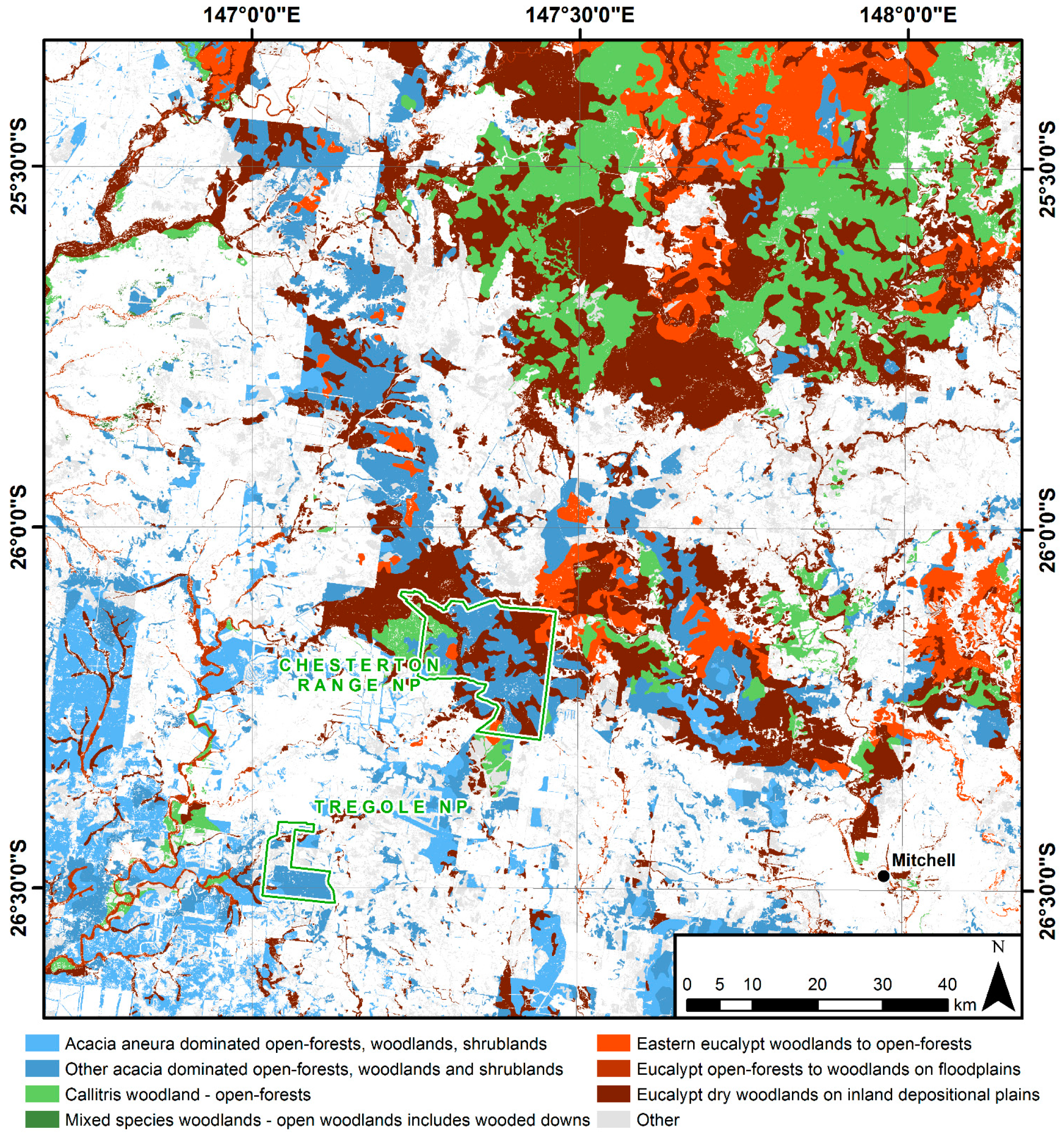
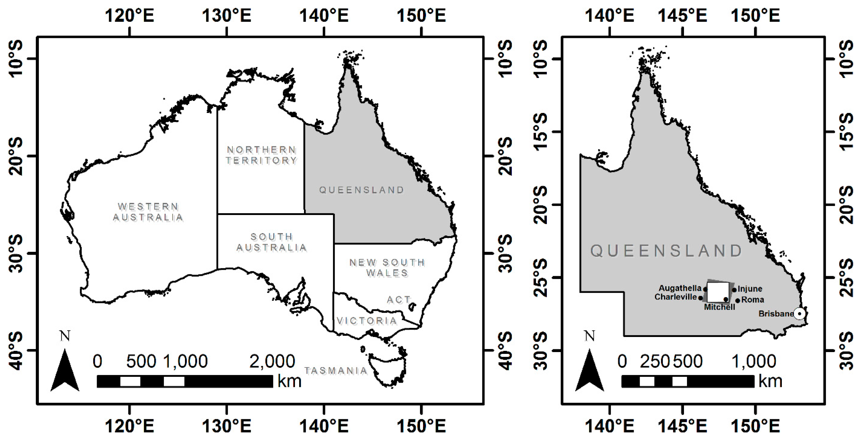
2. Study Area
3. Data
3.1. Landsat Data
3.2. MODIS Data
3.3. Reference and Auxiliary Datasets
4. Methods
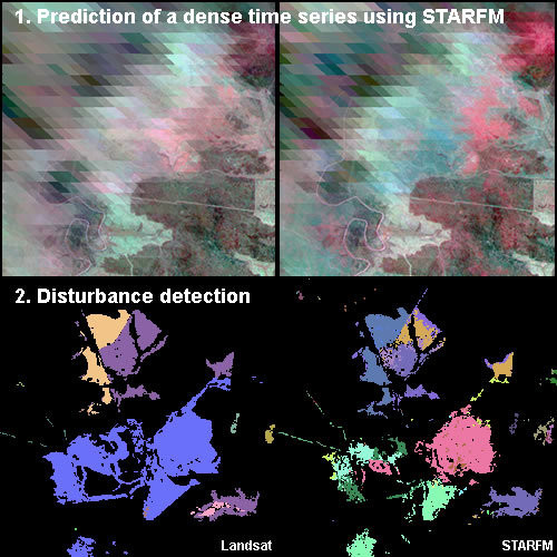
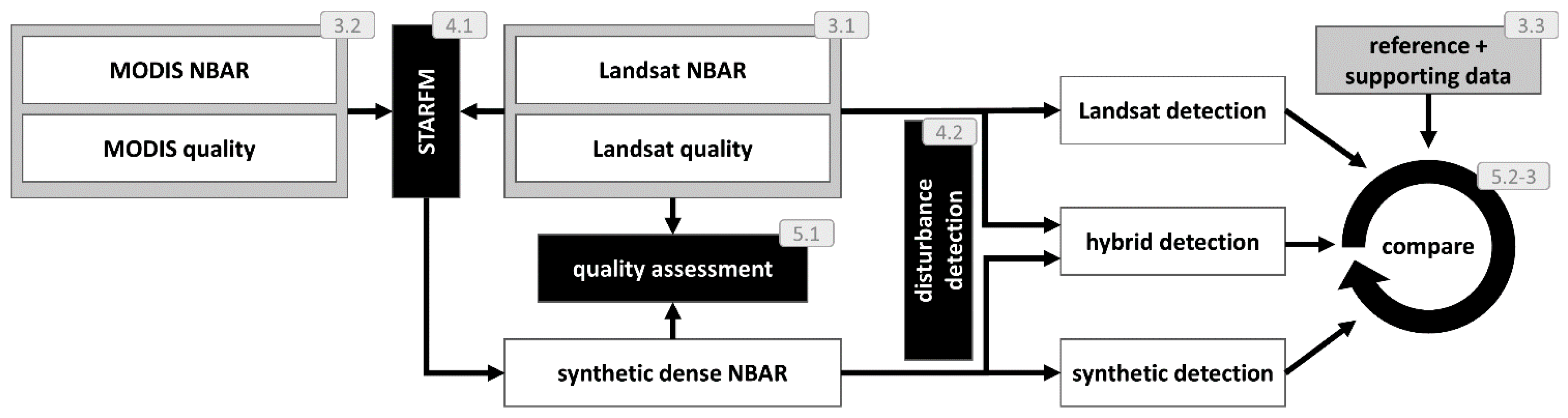
4.1. Prediction of a Dense Time Series
4.2. Disturbance Detection
- (i)
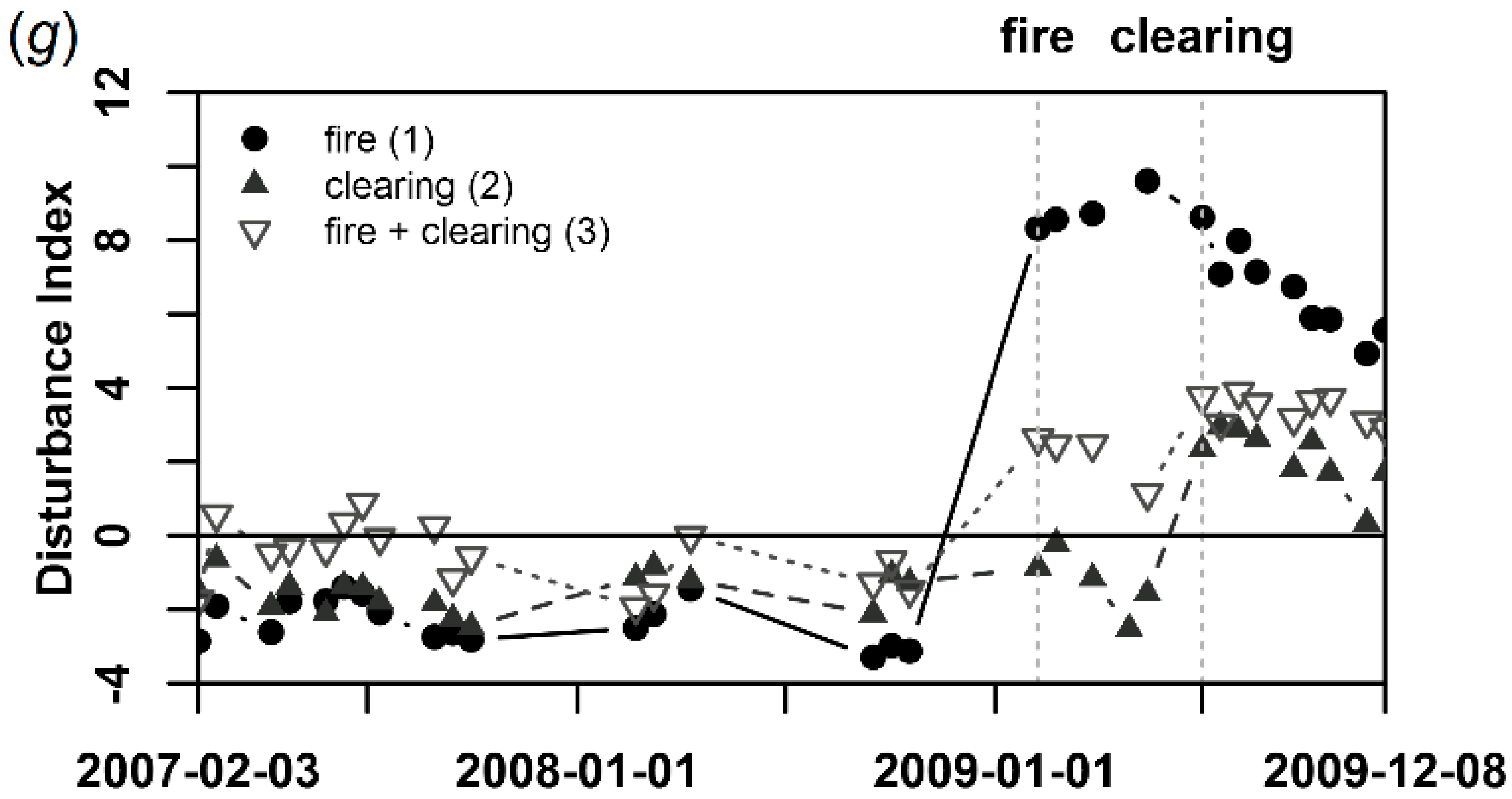
- Data transformation. Our approach is based on the analysis of temporal trajectories of the Disturbance Index (DI) transformation, which was developed to separate completely deforested areas from forest regions [24]. It is a linear transformation of the rescaled Tasseled Cap indices [28,43,44]:where the rescaled indices Xr are computed by normalizing the respective index X (brightness B, greenness G and wetness W) with the mean μ and standard deviation σ of a reference population:
- (ii)
- Temporal filtering. The DI time series might be noise affected, e.g., due to undetected cloud remnants. We eliminate positive spikes above a DI of 0.5 and thereafter negative spikes below or equal to zero. A spike is considered an observation that exceeds the threshold, whereas the bracketing data points are inconspicuous. Disturbances normally trigger a persistent DI response for a longer period. Positive spikes result in false positives if not removed (e.g., remnant clouds). Similarly, observations following a negative spike can also result in false positives. In the case of dense synthetic imagery, we apply an additional Savitzky–Golay filter [45] to smooth the DI time series and to lessen the noise that results from prediction errors.
- (iii)
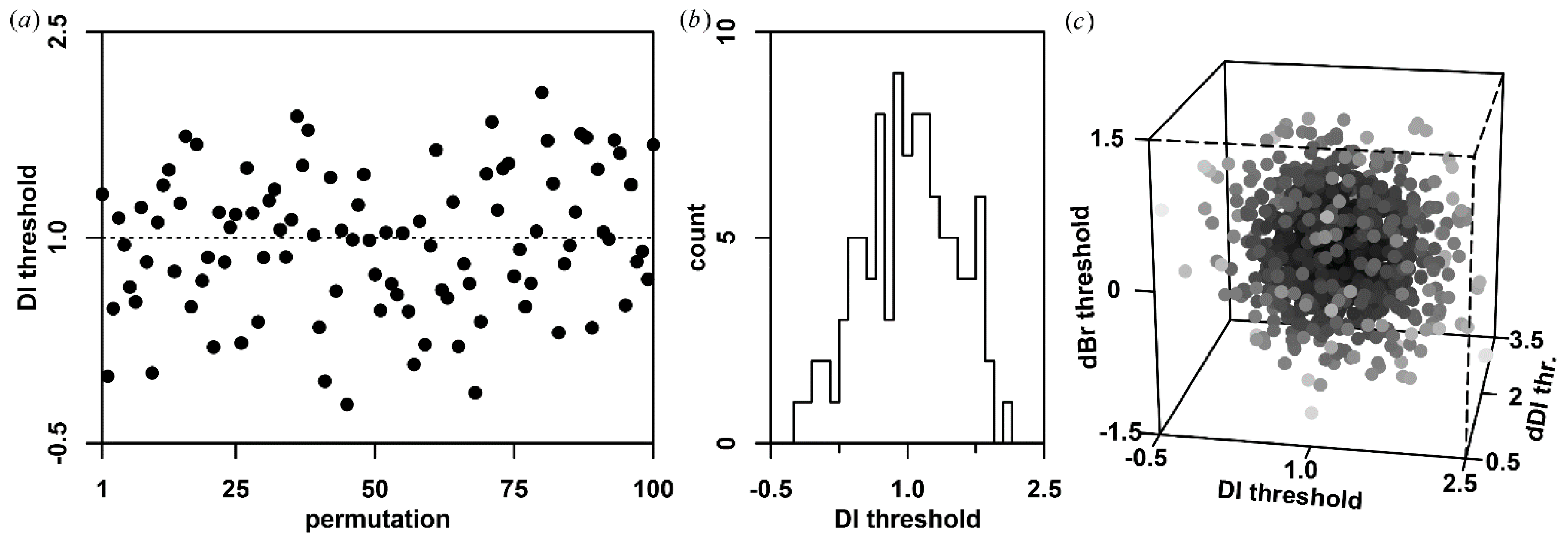
- Multi-temporal disturbance detection. A threshold-dependent rule set is used to identify potential disturbance events. A potential disturbance at time t is flagged if
- DI(t) exceeds a threshold DIT and
- the increase in DI (i.e., ΔDI(t) = DI(t) − DI(t − 1)) is larger than ΔDIT and
- Br(t) has increased by more than ΔBr,T and
- Wr(t) has decreased by more than ΔWr,T and
- NDVIr(t) (computed analogous to Equation (2)) has decreased by more than ΔNDVIr,T.
- (iv)
- Spatial filtering. After identifying disturbance events in the temporal sequence, each disturbance mask (binary image; 1 = disturbed, 0 = stable forest) at time t is spatially filtered. Disturbed pixels are rejected if none of their eight neighbors are disturbed in order to reduce outlier-induced noise [23]. Undisturbed pixels are set to disturbed if at least five neighbors are disturbed because they are likely also disturbed. Finally, the disturbance masks are segmented and each disturbed object with an area smaller than a given threshold nmin is removed. This filter is suitable for further noise reduction, but has the contradicting effect on the identification of small and narrow linear disturbances. The latter two filters originate from the Fmask cloud and cloud shadow detection algorithm [37] which in terms of image processing is related to disturbance detection because it is essentially also a binary classification method.
- (v)
- Hybrid detection. We additionally implemented a hybrid detection that makes use of observed and synthesized data. The Landsat detection result is used as the starting point and provides irregularly spaced disturbance masks. For each identified disturbance, the part of the synthetic time series between the potential event and the foregoing date (denoted as time slice) is investigated in detail. Analogous to the standalone detections, the (i) DI transformation; (ii) temporal filtering; and (iii) permutation-based detection of disturbances is performed for the synthetic images in the time slice. If there is a synthetic image with a higher disturbance probability P(t), this date is recorded instead. For simplicity, we assume that only one disturbance may occur per time slice.
5. Results
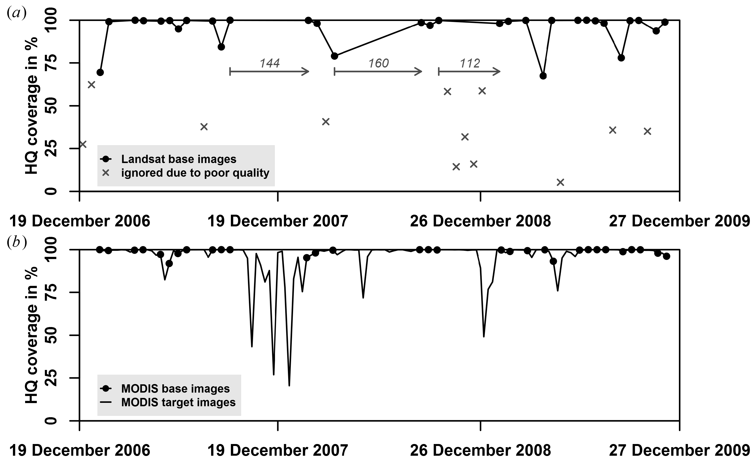
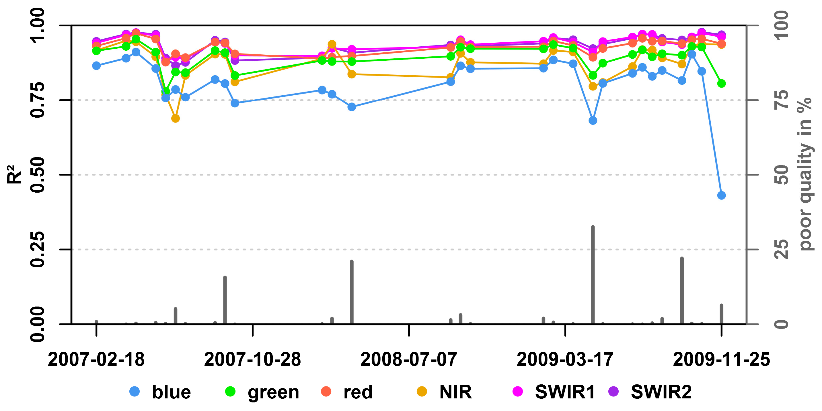
5.1. STARFM Quality Assessment
5.2. Landsat Disturbance Detection
5.3. STARFM Disturbance Detection
6. Discussion
6.1. STARFM Quality Assessment
6.2. Disturbance Index
6.3. Landsat Disturbance Detection
6.4. STARFM Disturbance Detection
- (i)
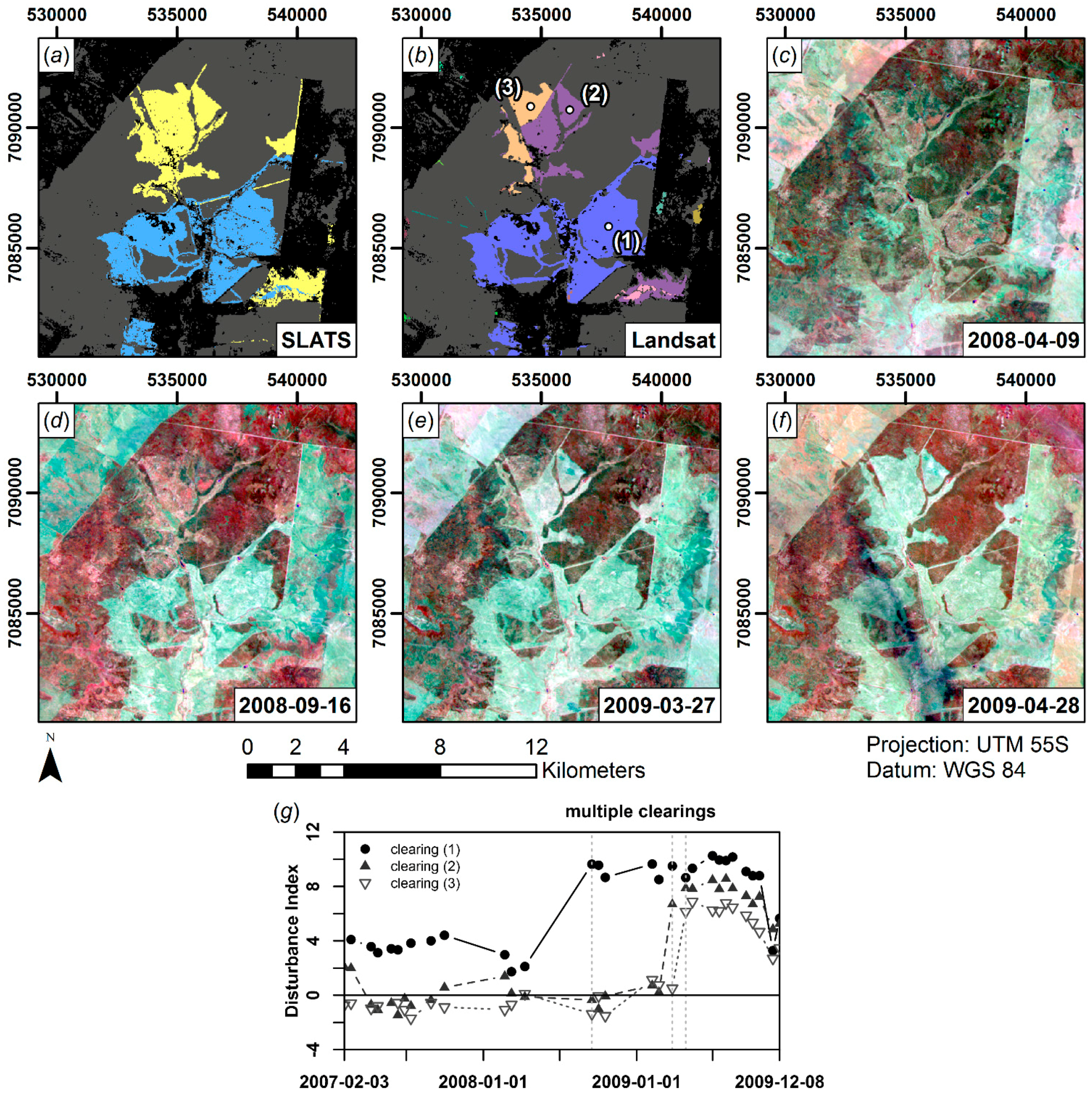
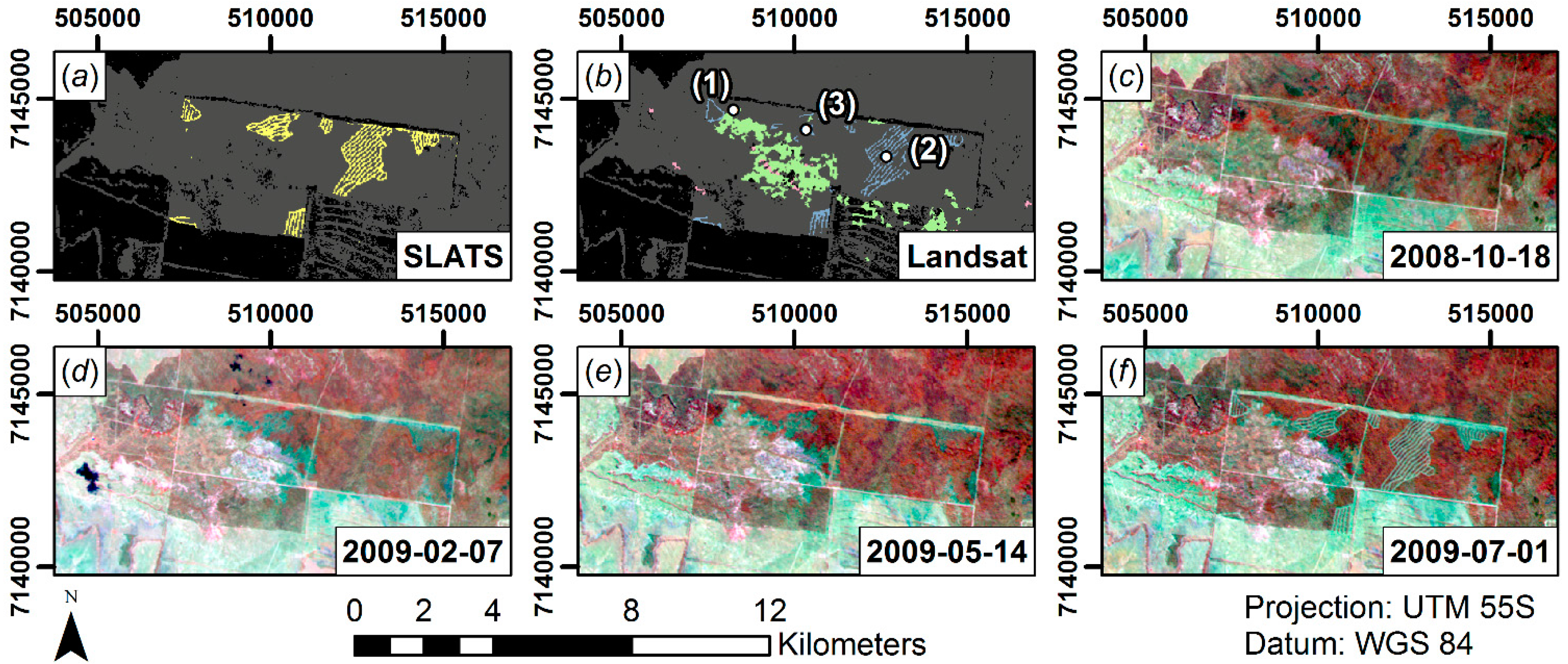
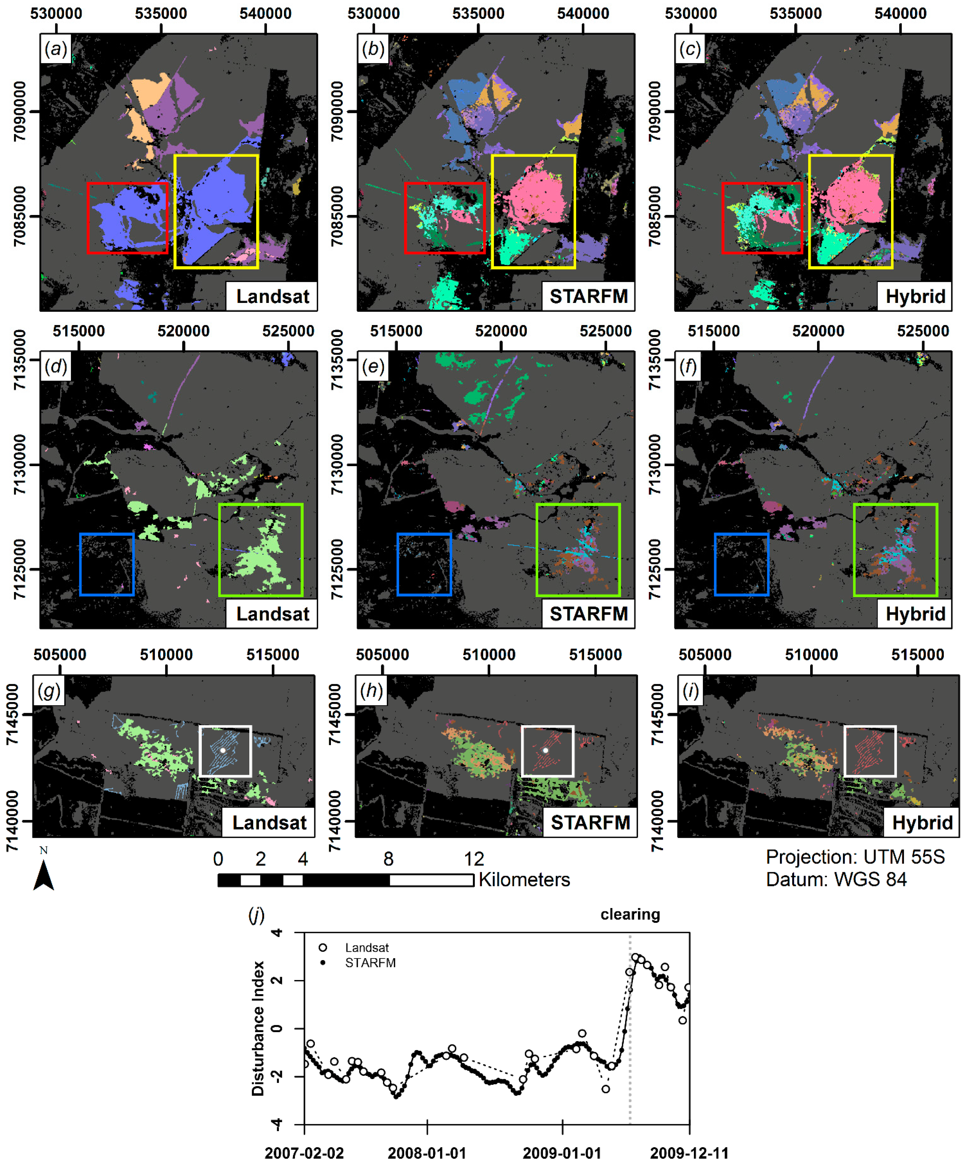
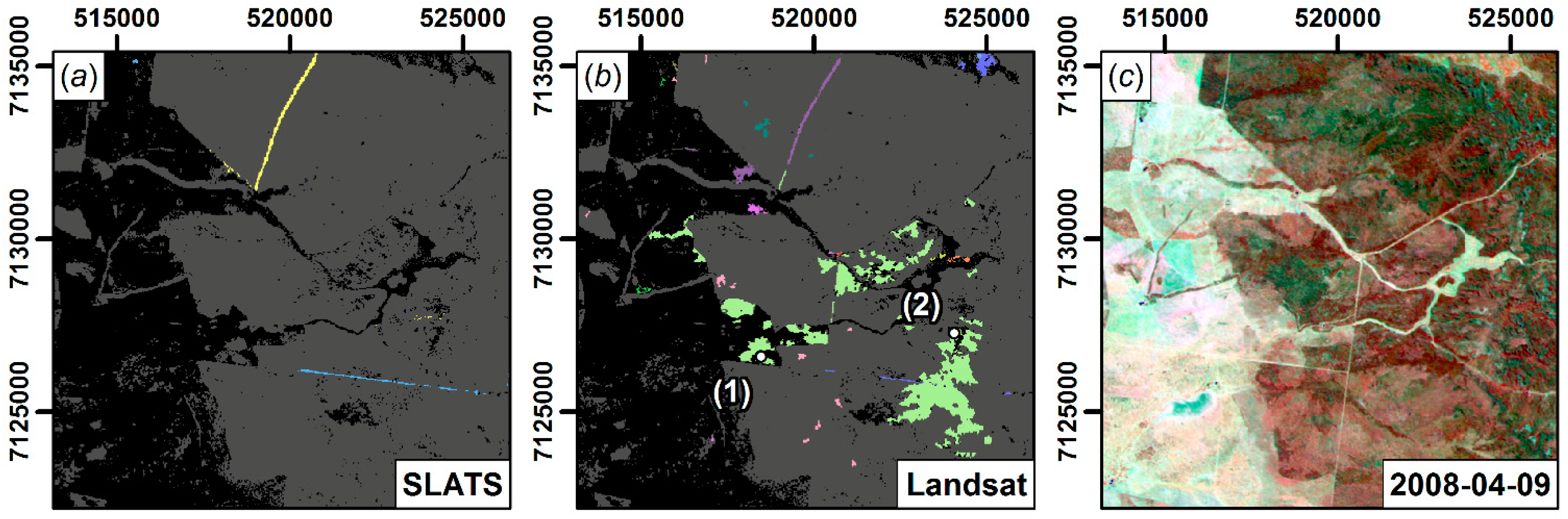
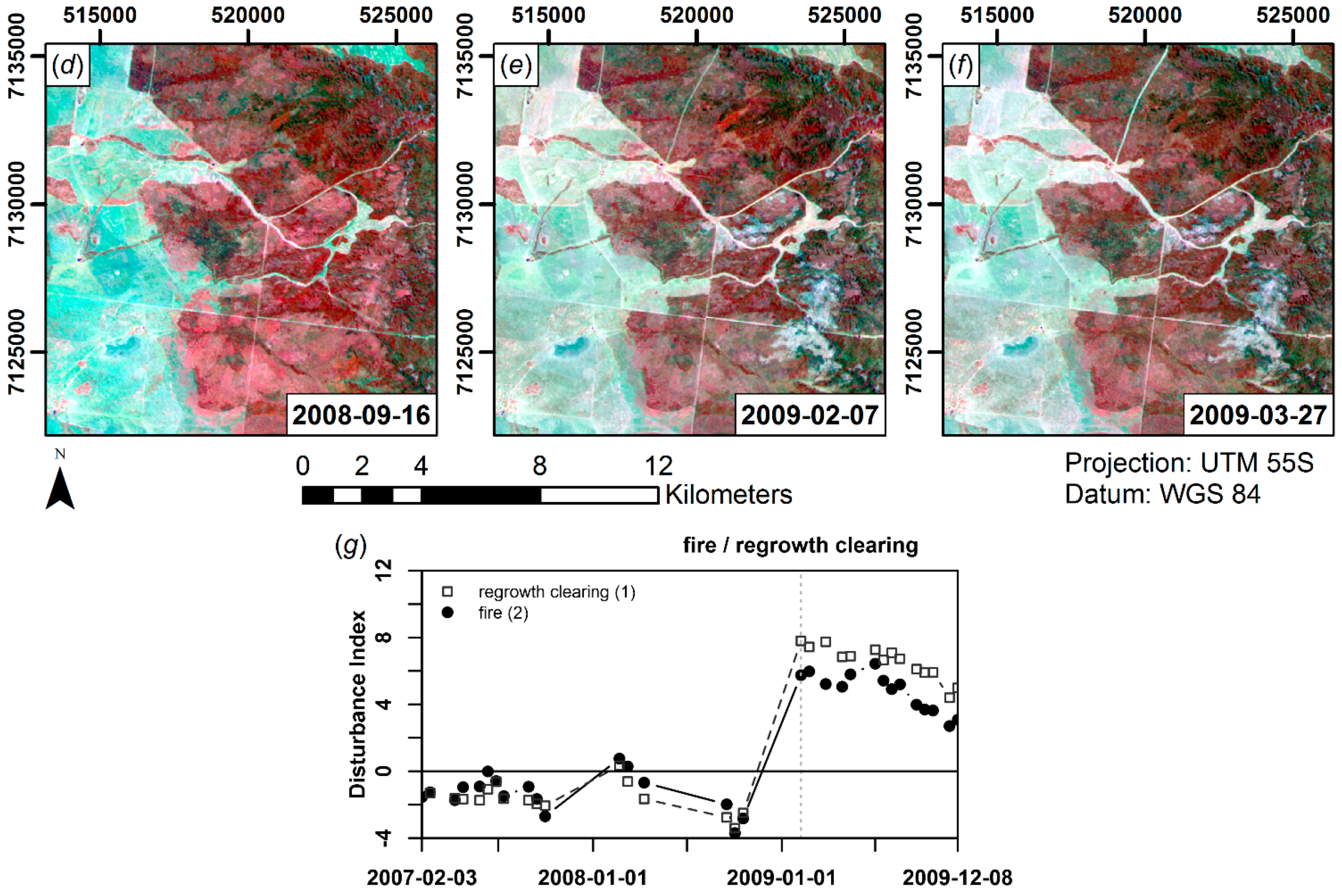
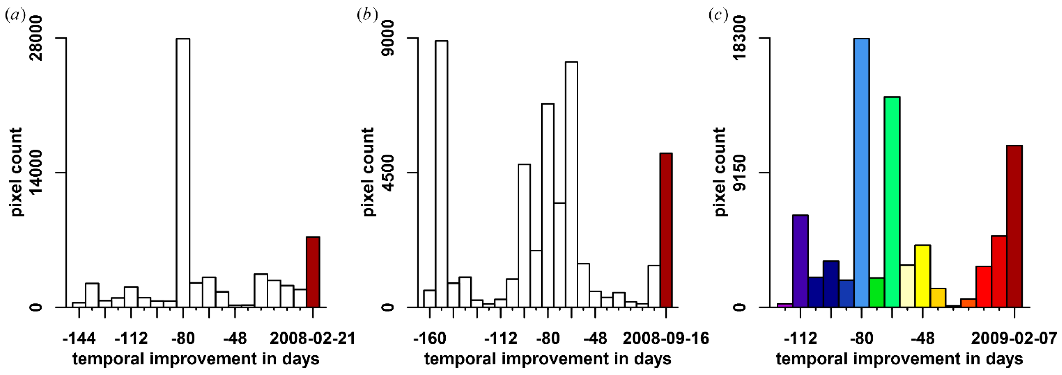
- Synthetic time series stand-alone detection. The higher temporal diversity in the STARFM product could indicate that there were indeed several clearing stages with high temporal frequency. This would be a substantial asset for state legislation as a detailed temporal documentation of the clearing succession is needed in cases of illegal logging [50]. On the contrary, the partially noisy appeal of disturbance timing could rather point to uncertainties in the STARFM prediction. It is hard to assess which process is true or if both factors are evident. In a local temporal window around each clearing event, the latter process seems to be certainly true, though. The boundaries of adjacent dates are somewhat diffuse and tend to become blurred and mixed up within one patch (e.g., Figure 10b red box; 25 June 2008: dark green, 3 July 2008: light-green, 11 July 2008: pink). This implies that the synthetic images might be useful to detect disturbance/clearing patches, but not at the full temporal resolution. One option might be to declare a detection uncertainty in temporal terms, e.g., ±8 days or ±16 days. Secondly, one could aggregate the results to a lower temporal frequency, e.g., to fortnightly or monthly time steps, which in many cases would still be an improvement to sparse Landsat data. On the contrary, there seem to be disturbed patches that could indeed be of different dates (e.g., Figure 10b yellow box; green: 9 June 2008; pink: 11 July 2008), because there is a sharp temporal and spatial boundary between the two polygon parts. As no reference data were available at an appropriate temporal scale, this proposition cannot be falsified or verified at the moment.
- (ii)
- Hybrid detection. The hybrid detection was characterized by coherent patches as in the Landsat detection, but additionally favored from increased temporal detail of the synthetic time series. Some pixels were characterized by no or little shift in disturbance timing. Thus, the timing either could not be improved with dense synthetic images or the discrete Landsat images were captured at the optimal point in time by chance. Figure 12 displays the major disturbances for the time slice shown in Figure 11c. The non-improved pixels are merely situated at the edge of patches or are small objects, which indicate that STARFM was not able to extract useful information (regarding land cover change) from the subtle MODIS reflectance change at a coarse spatial scale—as discussed in Figure 12i.
7. Conclusions
Acknowledgments
Author Contributions
Conflicts of Interest
Appendix


References
- Van der Werf, G.R.; Morton, D.C.; DeFries, R.S.; Olivier, J.G.J.; Kasibhatla, P.S.; Jackson, R.B.; Collatz, G.J.; Randerson, J.T. CO2 emissions from forest loss. Nat. Geosci. 2009, 2, 737–738. [Google Scholar] [CrossRef]
- Le Quéré, C.; Moriarty, R.; Andrew, R.M.; Peters, G.P.; Ciais, P.; Friedlingstein, P.; Jones, S.D.; Sitch, S.; Tans, P.; Arneth, A.; et al. Global carbon budget 2014. Earth Syst. Sci. Data 2015, 7, 47–85. [Google Scholar] [CrossRef]
- Tucker, C.J. Red and photographic infrared linear combinations for monitoring vegetation. Remote Sens. Environ. 1979, 8, 127–150. [Google Scholar] [CrossRef]
- Danaher, T.; Scarth, P.; Armston, J.; Collett, L.; Kitchen, J.; Gillingham, S. Remote sensing of tree-grass systems: The eastern Australian woodlands. In Ecosystem Function in Savannas: Measurement and Modeling at Landscape to Global Scales; Hill, M.J., Hanan, N.P., Eds.; CRC Press: Boca Raton, FL, USA, 2010; pp. 175–194. [Google Scholar]
- Armston, J.D.; Denham, R.J.; Danaher, T.J.; Scarth, P.F.; Moffiet, T.N. Prediction and validation of foliage projective cover from Landsat-5 TM and Landsat-7 ETM+ imagery. J. Appl. Remote Sens. 2009, 3. [Google Scholar] [CrossRef]
- Kennedy, R.E.; Townsend, P.A.; Gross, J.E.; Cohen, W.B.; Bolstad, P.; Wang, Y.Q.; Adams, P. Remote sensing change detection tools for natural resource managers: Understanding concepts and tradeoffs in the design of landscape monitoring projects. Remote Sens. Environ. 2009, 113, 1382–1396. [Google Scholar] [CrossRef]
- Wulder, M.A.; Masek, J.G.; Cohen, W.B.; Loveland, T.R.; Woodcock, C.E. Opening the archive: How free data has enabled the science and monitoring promise of landsat. Remote Sens. Environ. 2012, 122, 2–10. [Google Scholar] [CrossRef]
- Yan, L.; Roy, D.P. Automated crop field extraction from multi-temporal web enabled Landsat data. Remote Sens. Environ. 2014, 144, 42–64. [Google Scholar] [CrossRef]
- Baumann, M.; Kuemmerle, T.; Elbakidze, M.; Ozdogan, M.; Radeloff, V.C.; Keuler, N.S.; Prishchepov, A.V.; Kruhlov, I.; Hostert, P. Patterns and drivers of post-socialist farmland abandonment in western Ukraine. Land Use Policy 2011, 28, 552–562. [Google Scholar] [CrossRef]
- Gao, F.; Masek, J.; Schwaller, M.; Hall, F. On the blending of the Landsat and MODIS surface reflectance: Predicting daily Landsat surface reflectance. IEEE Trans. Geosci. Remote Sens. 2006, 44, 2207–2218. [Google Scholar]
- Roy, D.P.; Ju, J.; Lewis, P.; Schaaf, C.; Gao, F.; Hansen, M.; Lindquist, E. Multi-temporal MODIS-Landsat data fusion for relative radiometric normalization, gap filling, and prediction of Landsat data. Remote Sens. Environ. 2008, 112, 3112–3130. [Google Scholar] [CrossRef]
- Zhu, X.; Chen, J.; Gao, F.; Chen, X.; Masek, J.G. An enhanced spatial and temporal adaptive reflectance fusion model for complex heterogeneous regions. Remote Sens. Environ. 2010, 114, 2610–2623. [Google Scholar] [CrossRef]
- Hilker, T.; Wulder, M.A.; Coops, N.C.; Seitz, N.; White, J.C.; Gao, F.; Masek, J.G.; Stenhouse, G. Generation of dense time series synthetic Landsat data through data blending with MODIS using a spatial and temporal adaptive reflectance fusion model. Remote Sens. Environ. 2009, 113, 1988–1999. [Google Scholar] [CrossRef]
- Watts, J.D.; Powell, S.L.; Lawrence, R.L.; Hilker, T. Improved classification of conservation tillage adoption using high temporal and synthetic satellite imagery. Remote Sens. Environ. 2011, 115, 66–75. [Google Scholar] [CrossRef]
- Walker, J.J.; de Beurs, K.M.; Wynne, R.H.; Gao, F. Evaluation of Landsat and MODIS data fusion products for analysis of dryland forest phenology. Remote Sens. Environ. 2012, 117, 381–393. [Google Scholar] [CrossRef]
- Schmidt, M.; Udelhoven, T.; Gill, T.; Röder, A. Long term data fusion for a dense time series analysis with MODIS and Landsat imagery in an Australian Savanna. J. Appl. Remote Sens. 2012, 6, 063512. [Google Scholar]
- Bhandari, S.; Phinn, S.; Gill, T. Preparing landsat image time series (LITS) for monitoring changes in vegetation phenology in Queensland, Australia. Remote Sens. 2012, 4, 1856–1886. [Google Scholar] [CrossRef]
- Schmidt, M.; Lucas, R.; Bunting, P.; Verbesselt, J.; Armston, J. Multi-resolution time series imagery for forest disturbance and regrowth monitoring in Queensland, Australia. Remote Sens. Environ. 2015, 158, 156–168. [Google Scholar] [CrossRef]
- Verbesselt, J.; Hyndman, R.; Newnham, G.; Culvenor, D. Detecting trend and seasonal changes in satellite image time series. Remote Sens. Environ. 2010, 114, 106–115. [Google Scholar] [CrossRef]
- Tewes, A.; Thonfeld, F.; Schmidt, M.; Oomen, R.; Zhu, X.; Dubovyk, O.; Menz, G.; Schellberg, J. Using rapideye and MODIS data fusion to monitor vegetation dynamics in semi-arid rangelands in South Africa. Remote Sens. 2015, 7, 6510–6534. [Google Scholar] [CrossRef]
- Fu, D.; Chen, B.; Wang, J.; Zhu, X.; Hilker, T. An improved image fusion approach based on enhanced spatial and temporal the adaptive reflectance fusion model. Remote Sens. 2013, 5, 6346–6360. [Google Scholar] [CrossRef]
- Emelyanova, I.V.; McVicar, T.R.; Van Niel, T.G.; Li, L.T.; van Dijk, A.I.J.M. Assessing the accuracy of blending landsat-MODIS surface reflectances in two landscapes with contrasting spatial and temporal dynamics: A framework for algorithm selection. Remote Sens. Environ. 2013, 133, 193–209. [Google Scholar] [CrossRef]
- Hilker, T.; Wulder, M.A.; Coops, N.C.; Linke, J.; McDermid, G.; Masek, J.G.; Gao, F.; White, J.C. A new data fusion model for high spatial- and temporal-resolution mapping of forest disturbance based on Landsat and MODIS. Remote Sens. Environ. 2009, 113, 1613–1627. [Google Scholar] [CrossRef]
- Healey, S.P.; Cohen, W.B.; Zhiqiang, Y.; Krankina, O.N. Comparison of tasseled cap-based Landsat data structures for use in forest disturbance detection. Remote Sens. Environ. 2005, 97, 301–310. [Google Scholar] [CrossRef]
- Healey, S.P.; Yang, Z.; Cohen, W.B.; Pierce, D.J. Application of two regression-based methods to estimate the effects of partial harvest on forest structure using Landsat data. Remote Sens. Environ. 2006, 101, 115–126. [Google Scholar] [CrossRef]
- Masek, J.G.; Huang, C.; Wolfe, R.; Cohen, W.; Hall, F.; Kutler, J.; Nelson, P. North American forest disturbance mapped from a decadal Landsat record. Remote Sens. Environ. 2008, 112, 2914–2926. [Google Scholar] [CrossRef]
- Zhu, Z.; Woodcock, C.E.; Olofsson, P. Continuous monitoring of forest disturbance using all available Landsat imagery. Remote Sens. Environ. 2012, 122, 75–91. [Google Scholar] [CrossRef]
- Kauth, R.J.; Thomas, G. The Tasselled Cap—A Graphic Description of the Spectral-Temporal Development of Agricultural Crops as Seen by Landsat; LARS Symposia: West Lafayette, US, 1976; p. 159. [Google Scholar]
- Lucas, R.M.; Cronin, N.; Lee, A.; Moghaddam, M.; Witte, C.; Tickle, P. Empirical relationships between airsar backscatter and LiDAR-derived forest biomass, Queensland, Australia. Remote Sens. Environ. 2006, 100, 407–425. [Google Scholar] [CrossRef]
- Neldner, V.J.; Wilson, B.A.; Thompson, E.J.; Dilleward, H.A. Methodology for Survey and Mapping of Regional Ecosystems and Vegetation Communities in Queensland, Version 3.2.; Queensland Herbarium, Department of Science, Information Technology, Innovation and the Arts: Brisbane, Australia, 2012; p. 124.
- Specht, R.L. Foliage projective covers of overstorey and understorey strata of mature vegetation in Australia. Aust. J. Ecol. 1983, 8, 433–439. [Google Scholar] [CrossRef]
- Cowie, B.A.; Thornton, C.M.; Radford, B.J. The brigalow catchment study: I*. Overview of a 40-year study of the effects of land clearing in the brigalow bioregion of Australia. Soil Res. 2007, 45, 479–495. [Google Scholar] [CrossRef]
- Lucas, R.M.; Cronin, N.; Moghaddam, M.; Lee, A.; Armston, J.; Bunting, P.; Witte, C. Integration of radar and Landsat-derived foliage projected cover for woody regrowth mapping, Queensland, Australia. Remote Sens. Environ. 2006, 100, 388–406. [Google Scholar] [CrossRef]
- Harris, M.R.; Lamb, D.; Erskine, P.D. An investigation into the possible inhibitory effects of white cypress pine (Callitris glaucophylla) litter on the germination and growth of associated ground cover species. Aust. J. Bot. 2003, 51, 93–102. [Google Scholar] [CrossRef]
- Wulder, M.A.; White, J.C.; Masek, J.G.; Dwyer, J.; Roy, D.P. Continuity of Landsat observations: Short term considerations. Remote Sens. Environ. 2011, 115, 747–751. [Google Scholar] [CrossRef]
- Flood, N.; Danaher, T.; Gill, T.K.; Gillingham, S.S. An operational scheme for deriving standardised surface reflectance from Landsat TM/ETM+ and SPOT HRG imagery for eastern Australia. Remote Sens. 2013, 5, 83–109. [Google Scholar] [CrossRef]
- Zhu, Z.; Woodcock, C.E. Object-based cloud and cloud shadow detection in Landsat imagery. Remote Sens. Environ. 2012, 118, 83–94. [Google Scholar] [CrossRef]
- Frantz, D.; Roder, A.; Udelhoven, T.; Schmidt, M. Enhancing the detectability of clouds and their shadows in multitemporal dryland Landsat imagery: Extending Fmask. IEEE Geosci. Remote Sens. Lett. 2015, 12, 1242–1246. [Google Scholar] [CrossRef]
- Schaaf, C.B.; Gao, F.; Strahler, A.H.; Lucht, W.; Li, X.; Tsang, T.; Strugnell, N.C.; Zhang, X.; Jin, Y.; Muller, J.-P.; et al. First operational BRDF, albedo nadir reflectance products from MODIS. Remote Sens. Environ. 2002, 83, 135–148. [Google Scholar] [CrossRef]
- Statewide Landcover and Trees Study. Available online: https://www.qld.gov.au/environment/land/vegetation/mapping/slats/ (accessed on 31 January 2016).
- Queensland Government. Vegetation Management Act 1999. Available online: https://www.legislation.qld.gov.au/legisltn/current/v/vegetmana99.pdf (accessed on 31 January 2016).
- Tulleken, H. Poisson disk sampling. Dev. Mag. 2008, 21, 21–25. [Google Scholar]
- Crist, E.P.; Cicone, R.C. A physically-based transformation of thematic mapper data—The TM tasseled cap. IEEE Trans. Geosci. Remote Sens. 1984, GE-22, 256–263. [Google Scholar] [CrossRef]
- Crist, E.P. A TM tasseled cap equivalent transformation for reflectance factor data. Remote Sens. Environ. 1985, 17, 301–306. [Google Scholar] [CrossRef]
- Press, W.H.; Teukolsky, S.; Vetterling, W.; Flannery, B. Numerical Recipes in Fortran: The Art of Scientific Computing, 2nd ed.; University Press: Cambridge, UK, 1992. [Google Scholar]
- Luo, Y.; Trishchenko, A.P.; Khlopenkov, K.V. Developing clear-sky, cloud and cloud shadow mask for producing clear-sky composites at 250-m spatial resolution for the seven MODIS land bands over Canada and North America. Remote Sens. Environ. 2008, 112, 4167–4185. [Google Scholar] [CrossRef]
- Gillingham, S.S.; Flood, N.; Gill, T.K.; Mitchell, R.M. Limitations of the dense dark vegetation method for aerosol retrieval under Australian conditions. Remote Sens. Lett. 2011, 3, 67–76. [Google Scholar] [CrossRef]
- Cohn, J.S.; Lunt, I.D.; Ross, K.A.; Bradstock, R.A. How do slow-growing, fire-sensitive conifers survive in flammable Eucalypt woodlands? J. Veg. Sci. 2011, 22, 425–435. [Google Scholar] [CrossRef]
- Scarth, P.; Röder, A.; Schmidt, M.; Denham, R. Tracking grazing pressure and climate interaction—The role of Landsat fractional cover in time series analysis. In Proceedings of the 15th Australasian Remote Sensing and Photogrammetry Conference, Alice Springs, Australia, 13–17 September 2010; The Remote Sensing and Photogrammetry Commission of the Spatial Sciences Institute: Canberra, Australia, 2010. [Google Scholar]
- Goulevitch, B. Ten years of using earth observation data in support of Queensland’s vegetation management framework. In Evidence from Earth Observation Satellites; Purdy, R., Leung, D., Eds.; Brill: Leiden, The Netherlands, 2012. [Google Scholar]


| DIT | ΔDIT | ΔBr,T | ΔWr,T | ΔNDVIr,T | w | PT | nmin | ||
|---|---|---|---|---|---|---|---|---|---|
| Landsat | 1 | 2 | 0 | −0.5 | 0 | 5 | 75 | 10 | |
| STARFM | 0.75 | 0.75 | 0 | −0.5 | 0 | 11 | 20 | 5 | |
| hybrid | step 1 | 1 | 2 | 0 | −0.5 | 0 | 5 | 75 | 10 |
| step 2 | 0.75 | 0.75 | 0 | −0.5 | 0 | - | - | - |
| This Study | Bhandari et al., 2012 [17] | Watts et al., 2011 [14] | Hilker et al., 2009 [13] | Walker et al., 2012 [15] | |
|---|---|---|---|---|---|
| Red R2 | 0.93 | 0.86 | 0.55 | 0.54 | 0.94 |
| NIR R2 | 0.88 | 0.81 | 0.65 | 0.76 | 0.84 |
| Study area | Queensland, AU | Queensland, AU | Montana, USA | British Columbia, CAN | Arizona, USA |
| Aridity | dry | dry | dry | humid | dry |
| Landsat radiometry | NBAR. | Surface refl. | TOA refl. | Surface refl. | Surface refl. |
© 2016 by the authors; licensee MDPI, Basel, Switzerland. This article is an open access article distributed under the terms and conditions of the Creative Commons by Attribution (CC-BY) license (http://creativecommons.org/licenses/by/4.0/).
Share and Cite
Frantz, D.; Röder, A.; Udelhoven, T.; Schmidt, M. Forest Disturbance Mapping Using Dense Synthetic Landsat/MODIS Time-Series and Permutation-Based Disturbance Index Detection. Remote Sens. 2016, 8, 277. https://doi.org/10.3390/rs8040277
Frantz D, Röder A, Udelhoven T, Schmidt M. Forest Disturbance Mapping Using Dense Synthetic Landsat/MODIS Time-Series and Permutation-Based Disturbance Index Detection. Remote Sensing. 2016; 8(4):277. https://doi.org/10.3390/rs8040277
Chicago/Turabian StyleFrantz, David, Achim Röder, Thomas Udelhoven, and Michael Schmidt. 2016. "Forest Disturbance Mapping Using Dense Synthetic Landsat/MODIS Time-Series and Permutation-Based Disturbance Index Detection" Remote Sensing 8, no. 4: 277. https://doi.org/10.3390/rs8040277
APA StyleFrantz, D., Röder, A., Udelhoven, T., & Schmidt, M. (2016). Forest Disturbance Mapping Using Dense Synthetic Landsat/MODIS Time-Series and Permutation-Based Disturbance Index Detection. Remote Sensing, 8(4), 277. https://doi.org/10.3390/rs8040277