Abstract
We present the first comparison between new fAPAR and LAI products derived from the GlobAlbedo dataset and the widely-used MODIS fAPAR and LAI products. The GlobAlbedo-derived products are produced using a 1D two-stream radiative transfer (RT) scheme designed explicitly for global parameter retrieval from albedo, with consistency between RT model assumptions and observations, as well as with typical large-scale land surface model RT schemes. The approach does not require biome-specific structural assumptions (e.g., cover, clumping, understory), unlike more detailed 3D RT model approaches. GlobAlbedo-derived values of fAPAR and LAI are compared with MODIS values over 2002–2011 at multiple flux tower sites within selected biomes, over 1200 × 1200 km regions and globally. GlobAlbedo-derived fAPAR and LAI values are temporally more stable than the MODIS values due to the smoothness of the underlying albedo, derived via optimal estimation (assimilation) using an a priori estimate of albedo derived from an albedo “climatology” (composited multi-year albedo observations). Parameters agree closely in timing but with GlobAlbedo values consistently lower than MODIS, particularly for LAI. Larger differences occur in winter (when values are lower) and in the Southern hemisphere. Globally, we find that: GlobAlbedo-derived fAPAR is ~0.9–1.01 × MODIS fAPAR with an intercept of ~0.03; GlobAlbedo-derived LAI is ~0.6 × MODIS LAI with an intercept of ~0.2. Differences arise due to the RT model assumptions underlying the products, meaning care is required in interpreting either set of values, particularly when comparing to fine-scale ground-based estimates. We present global transformations between GlobAlbedo-derived and MODIS products.
1. Introduction
Estimating structural and radiometric properties of terrestrial vegetation is a key aim for Earth Observation (EO) studies from local to global scales. Consistent estimates of LAI and fAPAR at these scales are also a requirement for improved land surface models (LSMs) [1]. Vegetation structure and amount is widely-characterized by the canopy leaf area index (LAI); radiometric properties of vegetation (absorption in particular) are related to the fraction of absorbed photosynthetically active radiation (fAPAR). LAI encapsulates the amount of vegetation available for radiation absorption, while fAPAR describes the efficiency of absorption. As a result, a wide range of approaches has been developed to estimate these properties from satellite observations of reflected radiation [2,3]. These approaches range from the purely empirical, exploiting relationships between fAPAR and LAI and easily estimated spectral indices such as normalised vegetation index (NDVI) [4], to physically-based radiative transfer (RT) models that describe reflected solar radiation as a function of LAI and fAPAR [5,6]. Key advantages of the physically-based approach are that it is quantitative and allows for attribution of changes in the observed signal to changes in the surface properties. Just as importantly, the uncertainty in the resulting parameter estimates can be characterized explicitly (although this is not always done in practice). Physically-based RT model retrievals underpin the most widely-used LAI and fAPAR estimates, such as those derived from the NASA MODIS instruments [7,8].
Here, we describe the properties of a new LAI and fAPAR product, derived from estimates of broadband albedo rather than spectral reflectance using an optimal model-observation framework. The underlying albedo data were developed for the European Space Agency (ESA) GlobAlbedo project [9]. The LAI and fAPAR products have been derived from GlobAlbedo products as part of the ESA Water Cycle Observation Multi-mission Strategy—EvapoTranspiration (WACMOS-II) project, to provide inputs into large-scale models of terrestrial evapotranspiration [10]. The key innovation of the approach is that the RT model inversion scheme underpinning it has been designed explicitly for parameter retrieval from global observations of albedo, in a suitable form for ingestion into terrestrial vegetation models. As a result, the assumptions underlying the retrieval scheme are consistent from the perspective of both observations and the resulting parameters.
Below, we present a brief discussion of definitions of LAI and fAPAR, including some caveats as to how they are interpreted in RT retrieval schemes. Following this, we outline the retrieval process (described in full elsewhere) and then provide details of the new GlobAlbedo-derived products. We then present a comparison between the resulting products and the MODIS LAI and fAPAR products at various scales, including at flux tower sites, across individual MODIS tiles (1200 × 1200 km) and across the entire northern and southern hemisphere land surfaces. We stress at the outset that these comparisons are not intended to try and establish which set of products is “right”; the impossibility of actually measuring LAI and fAPAR directly at anything other than trivially small scales rules this out. Our aim is in fact the opposite: we suggest that these comparisons illustrate where consistency between retrieval schemes can be expected and where not; they also highlight how different assumptions made in the retrieval process can be mistakenly interpreted as differences in land surface properties. We emphasize the need for clarity regarding model assumptions and explicit calculation of the resulting uncertainty.
1.1. Leaf Area Index (LAI)
LAI, in an ecological sense, is (typically) defined as the total canopy area per unit ground area (m2·m−2) [11] and ranges from 0 (bare ground) to over 10 (dense forest). LAI determines the interception of solar energy (and thus the fAPAR) for photosynthesis, as well as the available area for gas and water exchange between plant and atmosphere. LAI in a remote sensing sense, in contrast, is (typically) defined as one-sided leaf area per unit ground area (m2·m−2) i.e., 0.5 of the total [1,12], primarily from the point of view of light interception. Projected leaf area is often the more general requirement for radiation interception, which is dependent on leaf angle distribution [13,14]. Here, LAI is defined in the latter sense as half the total canopy area per unit ground area (m2·m−2).
Caveats: LAI
Despite the (seemingly) relatively simple and physically-meaningful definition of LAI given above, two key issues must be considered in practice when using LAI derived from EO data. The first is to do with the problem of relating LAI inferred from satellite data to other indirect estimates of LAI [15]; the second issue is to do with the scale at which observations are made.
LAI can only be measured directly via destructive harvest and scanning/weighing, which is impractical over anything other than very small areas (a few m2). Indirect methods are thus widely used to infer LAI, typically via upward-looking hemispherical photographs (hemiphotos) or bespoke instruments that compare light levels above and below the canopy (e.g., LI-COR LAI 2200c Plant Canopy Analyser [16]; the Delta-T SunScan Canopy Analysis System [17] and so on). In these cases, LAI is inferred based on assumptions of the canopy absorption properties (e.g., all canopy elements are black) and architecture (e.g., assuming the canopy is horizontally homogeneous, and/or leaf angle distribution is uniform or spherical) [18,19].
LAI (and fAPAR) estimates from EO data are typically made by inverting RT models against estimates of surface fluxes or albedos (e.g., visible and NIR albedo here), resulting in model parameter estimates of (inter alia) LAI and fAPAR. Note that EO-derived albedo values are not direct observations per se, but are model-derived values produced from angular samples (observations) of surface reflectance, interpolated over viewing and illumination angles and time via RT model schemes to provide hemispherical integral fluxes (GlobAlbedo Algorithm Theoretical Basis Document: ATBD, 2013). Ideally, assumptions underlying the RT schemes used for both generating albedo (or surface reflectance) and for LAI retrieval should be the same; however this is rarely the case in practice. To achieve consistency of this sort [20] suggest adopting an “effective” LAI () such that where is the domain averaged LAI, and is a structural term that encapsulates the fact that real canopies are not turbid media but are clumped at multiple scales (from 10−2 m within shoots, to 102 m at the stand level). Clumping acts to reduce compared to the true value, , as the degree of clumping increases. In contrast, very regular canopies (crops for example) will tend to have > [19,21].
The adoption of permits a solution to the 1D limiting case of RT in a 3D canopy that is consistent with the assumptions made in many surface flux retrievals, as well as in large-scale Earth System Models (ESMs) (e.g., see [1,22]). Using also allows the use of a relatively simple two-stream 1D RT scheme that can be applied to large (global) datasets. In this case, is then the equivalent of optical thickness. Crucially however, values of are not the same as , which in turn are not the same as the LAI that would be measured on the ground (unless measured over some large, discrete canopy volume). That is, the resulting is a model-dependent (effective) parameter that does not have a direct (physically-defined, measurable) meaning, but is determined via the inversion scheme such that observed fluxes can be reproduced by the RT scheme. The benefit is that this allows solution of the 1D RT problem by representing domain-averaged quantities that are forced to satisfy the constraints associated with a 1D representation of what is an inherently 3D system [20,23].
We emphasize this point about effective parameters to highlight the fact that care must be taken in comparing and interpreting LAI values derived from different sources: key assumptions should always be made explicit in a particular model or application, so differences can be quantified and/or accounted for (e.g., via cross-calibration/transformation of LAI values). This is particularly important when the resulting parameters are intended for wide use, and users may have little interest in the subtleties of how the parameters were estimated. In this case, it is crucial to explain how and why differences arise between indirect estimates from different sources, despite apparently being measurements of the same, seemingly well-defined physical quantity.
Here, LAI is derived from a two-stream inversion package (the JRC-TIP, outlined below) based on a 1D-equivalent LAI, for solving RT in a 3D medium. This is consistent with the method used to produce the albedo from which LAI is subsequently derived. It is not consistent with LAI derived using a more complex 3D RT scheme that allows some form of horizontal clumping (e.g., MODIS LAI), and will typically be lower than such a value. Neither of these EO-derived values is consistent with values measured in the field using indirect, optical methods at small scale. None of these indirect estimates are directly comparable with the real LAI that would be measured destructively. There is of course (fortunately) a high degree of correlation between these values. However, they still have to be locally calibrated, or generalised across biomes and scales (i.e., for a particular scale/type of clumping).
The second issue, that of scale, must also be considered when comparing LAI estimates, and is related to clumping. The authors of [24] discuss this issue, where the same total amount of leaf material (LAI) may be present in each case, but clearly the arrangement of the material (even in simple cases) will determine the radiometric response [23]. The authors of [24] also highlight how the scale of observation alters the information available from a measurement at aggregation from 0.1 m (~leaf scale) to 30 m (~stand scale). Much, if not all, of the information on the spatial arrangement of the canopy is lost in moving from the leaf to the stand scale, even down to the number of trees in the scene, yet the underlying “real” LAI is the same. Models which allow us to relate radiometric variables measured at one scale, to ecological (structural/radiometric) properties at a (usually) finer scale do not in general scale linearly across space, and nor should we expect them to [14,25]. A different approach has been to consider the EO parameter scaling issue from an information content perspective [26], as a possible alternative to simple aggregation.
1.2. fAPAR: Fraction of Absorbed Photosynthetically Active Radiation
Here, fAPAR is defined as the fraction of absorbed photosynthetically active radiation (PAR, 400–700 um). fAPAR is generally more straightforward to define than LAI, if not to measure. fAPAR is a dimensionless variable, varying between zero and one, and is related to the state and change of vegetation amount and productivity. The authors of [27] note that due to the requirement for consistent radiometric processing, it is difficult to generate long time series of fAPAR estimates due to inconsistencies between sensors and drifts in calibration of single sensors over time. In this study, it is produced in a step subsequent to the LAI retrieval procedure.
Caveats: fAPAR
fAPAR would seem, in principle, to be an even more straightforward property to define and hence to use and interpret than LAI. However, as for LAI, fAPAR derived from RT model inversion depends on the assumptions of the underlying model: fAPAR derived from a 1D RT model will not be directly comparable with that derived from a 3D model; in particular, magnitudes will likely be different. The authors of [28] discuss the issue of deriving so-called Essential Climate Variables (ECVs) from EO. They use fAPAR as an example ECV, pointing out that identifying fAPAR as an ECV has helped focus attention on retrieval, resulting in multiple fAPAR datasets, each generated using a slightly different approach. They note that there is no single central definitive archive or product, nor has such ever been proposed. The authors of [27] have also suggested ways to generate consistent fAPAR values from MERIS and SeaWIFS sensors, and note that although agreement is generally close, differences occur even though they are essentially calculated in the same way. Differences are likely due to outlier detection (cloud contamination), sensor and illumination view angle variations and underlying biases in each dataset.
Therefore, as for LAI whilst the definitions of fAPAR are apparently clear and unambiguous, EO-derived values are subject to the assumptions of retrieval and observation characteristics. This is of course the case for all EO-derived biophysical properties, even those which appear to be near-direct measurements such as surface temperature, surface reflectance and albedo. Here, the GlobAlbedo-derived estimates of fAPAR arise from the retrieval of LAI i.e., they are the values arising from the RT model-derived LAI values such that observed fluxes can be reproduced by the RT scheme. In this sense, the GlobAlbedo-derived fAPAR values are not “effective” in the sense of the LAI values as described above—they arise as a function of the LAI retrieval process.
In Section 2 below, a brief overview is given of the RT model retrieval scheme used to derive the GlobAlbedo fAPAR and LAI values, as well as a description of the site locations at which comparisons between the GlobAlbedo-derived and MODIS values are made. In Section 3, we present examples of the GlobAlbedo-derived LAI and fAPAR products at global scale, including retrieval uncertainties (In figures below the abbreviation GA signifies GlobAlbedo-derived values). We then show comparisons of the 1 km GlobAlbedo-derived LAI and fAPAR estimates with the corresponding MODIS LAI and fAPAR estimates over 2002–2011 at specific sites, selected to cover a wide range of different vegetation types and conditions. We then present regional (1200 × 1200 km tile) comparisons. Finally, we compare parameter distributions at the global scale for the Northern and Southern hemisphere, winter and summer.
2. Experimental Section
Here, we briefly outline the radiative transfer (RT) model inversion scheme used to derive the GlobAlbedo-based LAI and fAPAR data used in the analysis above. Following this we describe the data format, size and coverage. We then outline the MODIS LAI and fAPAR products against which the GlobAlbedo-derived LAI and fAPAR estimates are compared. Lastly, we describe the site locations at which the site-level comparisons between the GlobAlbedo-derived and MODIS LAI and fAPAR estimates are made.
2.1. GlobAlbedo-Derived LAI and fAPAR
LAI and fAPAR are derived from an inversion of a 1D RT scheme, the JRC Two Stream Inversion Package (JRC-TIP) against the GlobAlbedo albedo values in the VIS (400–700 nm) and NIR/SWIR (700–3000 nm) wavelengths. The latter is referred to hereafter as the NIR channel for the avoidance of doubt. These values are consistent with the underlying observations, but are not those that would be obtained from a 3D RT inversion scheme (due to clumping), nor would they be those measured on the ground. The RT theory underpinning the inversion scheme, and the implementation of this in the JRC-TIP are described in [29,30,31]. Generation of the albedo data underlying the LAI and fAPAR products is described in detail in the GlobAlbedo Algorithm Theoretical Basis Document [32]. A brief overview is provided below.
2.1.1. Two-Stream Model
The TIP is an inversion scheme explicitly developed for rapid, robust retrieval of surface variables (including LAI and fAPAR) from observations such as albedo, particularly at large spatial scales. The TIP approach makes use of effective parameters explicitly, in particular the LAI is intended to be consistent with the 1D RT solution for deriving observed fluxes, rather than to be the most “realistic” estimate possible (unlike the MODIS LAI/fAPAR RT model scheme). One reason for taking this approach is that it is consistent with how radiation is treated in large-scale Earth System Models of climate and carbon cycle [22]. A second reason for using this approach is that it is driven entirely by the underlying observations, unlike 3D model schemes that account for variability in clumping and background properties by specifying biome-specific prior structural information to separate grasses, deciduous and evergreen tree types for example.
The approach proposed by [20] uses a standard two-stream approach allowing decomposition of the directional hemispherical reflectance field (DHR, ) emerging from the top of a canopy layer at depth into three terms:
where is the solar zenith angle. The terms on the RHS represent, respectively: , radiation that has interacted with the vegetation canopy elements only; radiation that has interacted with the soil only i.e., travelling uncollided both downwards and upwards through gaps in the canopy; and that has collided multiple times with both canopy and background. The major advantage of this approach (over a more detailed 3D approach for example) is that it can be solved analytically. The use of effective variables (for the canopy) guarantees the correct simulation of the scattered, transmitted and absorbed radiant fluxes. The authors of [20] derive values of the surface variables by inverting a 1D radiant flux model against fluxes generated by a 3D model. This guarantees accurate simulations of the three radiant fluxes when using, in direct mode, these effective values. In addition it does not require explicit consideration of other canopy elements (woody material) as these are considered implicitly in the diffuse (multiple scattered) fluxes. The resulting approach agrees well with 3D model simulations across a range of structural configurations [20].
2.1.2. Two-Stream Model Inversion
Inversion of the two-stream model is described in [29]. In brief, the process is a standard inversion via the minimization of a cost function of a vector of state variables (parameters) that quantifies the difference between model simulated fluxes given , , and observed fluxes, plus the deviation of from prior information on the state variables i.e.,
The parameters required by the TIP are the spectrally invariant LAI and the leaf single-scattering albedo , the leaf asymmetry factor and the background albedo and , for the visible and near-infrared spectral domains respectively. Note that only the canopy variables LAI, and are effective, in contrast to . By solving for the scattered and transmitted radiant fluxes, the absorbed component, fAPAR or , is given by considering energy closure in the case of a black (totally absorbing) background i.e., , where is simply the component transmitted by the vegetation through multiple interactions.
The model inversion problem is simplified by assuming observation and model parameter probability distributions are Gaussian, and using a locally-linear approximation of . In this case, the posterior probability distribution of model parameters can be represented as
where T represents the transpose operator; and are the mean and uncertainty covariance matrix of ; is the inverse of . The resulting minimizes the cost function . In practice, is minimized using a gradient descent method using the adjoint of . Uncertainty ranges for are approximated through inversion of the Hessian matrix of . The Jacobian matrix of first derivatives of fluxes with respect to parameters is used to propagate parameter uncertainty to flux uncertainty. All derivative code is derived via automatic differentiation of the code that implements [33,34].
The authors of [29] demonstrated the utility of the TIP in retrieving LAI and fAPAR from MODIS and MISR broadband surface albedo products. The authors of [30] demonstrated the performance of the TIP in deriving surface parameters on global scales from MODIS albedo data. In particular, they showed the benefits of the TIP scheme for the generation of physically consistent information about the density and absorbing properties of the vegetation layer together with the brightness of the background underneath. LAI values followed expected trajectories of seasonal and spatial distributions. The estimated uncertainties on LAI were strongly correlated with the LAI itself and to a lesser extent to the brightness of the underlying “soil” background.
The current product was generated with two different sets of prior information as in [31], to distinguish between snow and no snow background conditions for which the input albedo pairs were separately provided, together with a snow fraction. Four relative uncertainty values (5%, 7%, 10%, and 20%) were assigned to the albedo input pairs, respectively corresponding to GA product uncertainty values in the intervals (0, 5%], (5%, 7%], (7%, 10%] and (10%, infinity).
2.1.3. Spatial Resolution
GlobAlbedo-derived fAPAR and LAI data are produced at 3 separate resolutions: 1, 5 and 25 km. An important point is that the 5 km and 25 km data products are not simply aggregated versions of the 1 km products, but are produced from up-scaled albedo data. These data in turn are calculated from up-scaled bidirectional reflectance factor (BRF) data. This is done in the GlobAlbedo processing to ensure energy conservation in upscaling to each of these native resolutions. Simple aggregation cannot account for sub-pixel heterogeneity correctly (due to non-linearities in spatial scaling) and so the upscaled products are generated using underlying albedo data at the native resolution. Furthermore, simple aggregation would require the (variable) spatial covariance of the uncertainty, which is per se not available.
2.1.4. Data Format
GlobAlbedo-derived fAPAR and LAI products are provided in the NetCDF format [35] via the subsetting tool previously referred to. Data are stored using the MODIS SIN projection and tiling system [36]. The online data have 321 non-fill land tiles, each one of 1200 × 1200 1 km pixels (see below), 240 × 240 pixels at 5 km and 48 × 48 at 25 km.
2.1.5. Time Period and Data Size
GlobAlbedo-derived fAPAR and LAI products have been generated for the years 2002–2011, globally, at each separate resolution. For 1 tile of either LAI and fAPAR (and associated QA information), for 1 year at 1 km the data are ~400+ MB (with size varying substantially between tiles) and ~145 GB for 1 year globally; the 5 km and 25 km resolution datasets are ~4.3 GB and ~200 MB globally per year respectively. Snow-fraction areas are flagged in the processing during generation of the 1 km GlobAlbedo data, and are flagged and processed as such in the 5 km and 25 km aggregated data (i.e., the aggregation of snow pixels is considered at those lower resolutions).
2.1.6. FLUXNET Sites Used for Site-Level Comparisons
A range of sites were selected from the FLUXNET database [37], to allow comparisons of GlobAlbedo-derived and MODIS fAPAR and LAI products over key (wide global coverage) vegetation cover types, namely: grasslands, crops/natural, deciduous broadleaf, evergreen needleleaf, mixed forest. In addition we selected some miscellaneous sites in tropical and temperate regions. The locations for site comparisons were made from the FLUXNET database via their IGBP land use classifications (see [38]). The selected cover types are as follows:
- Grasslands
- Deciduous broadleaf
- Evergreen needleleaf
- Mixed forest
- Crop/natural
In each case the first four sites in site order were selected from the FLUXNET list of available sites in each land cover class, with complete MODIS and GlobAlbedo data coverage from 2002 to 2011. We also include four miscellaneous sites: Hainich (mixed forest) and Tharandt (evergreen needleleaf forest) in Europe; and 2 tropical deciduous broadleaf sites at Caxiuanã and Guyaflux. These are included to demonstrate the problems of parameter retrieval due to snow and cloud (Europe) or persistent cloud cover and even LAI saturation (tropics). Sites are listed below in Table 1, in each case with their FLUXNET site name, full name and location.

Table 1.
Site name, full name and location of the various FLUXNET sites used for comparison.
2.2. MODIS LAI and fAPAR
The MODIS LAI and fAPAR products are described in full in the Algorithm Theoretical Basis Document (ATBD) [8]. These data are perhaps the most widely-used global LAI and fAPAR products, in part due to being the only physically-based estimates of LAI and fAPAR derived using 3D RT model inversion [7,8]. The data used are the MODIS collection 6 products (released 2015) i.e., fAPAR and LAI derived from MODIS observations of surface reflectance, aggregated over 4 days (MCD15A2) from 1 km composites of observations, using data aggregated from MODIS sensors aboard both the Terra and Aqua platforms (collection 6 MCD15A2 product). MODIS data were obtained from [38]. Aggregation over time maximizes the chances of obtaining sufficient good quality (cloud free primarily) observations to allow model inversion, and assumes that the surface is stable over the aggregation period. 3D RT model inversion is via a look-up-table (LUT) containing pre-computed values of RT-modelled reflectance across a range of model parameter and observation configurations. The LUT is divided into 8 biome types, representing structurally different 3D vegetation canopy types. The resulting LAI and fAPAR values are provided at 1 km, with an associated uncertainty derived from the inversion scheme, and quality assurance (QA) flags indicating the quality of the inversion. Here we only consider values flagged as highest quality in the QA data. It is important to reiterate that when comparing between GlobAlbedo-derived and MODIS values we do not imply that either product is “right”; as described above, the products rely on different RT model (and processing) assumptions, and these are different from those used in field measurements using optical devices, which are in turn not the same as direct, destructive measurements (the only real answer).
Separate site-level comparisons are presented, for varying cover types across the globe. Sites from the FLUXNET database were selected, as these are well-characterized and studied over significant time periods. GlobAlbedo-derived LAI and fAPAR estimates were obtained through the GlobAlbedo website (see [39]) or direct via the GlobAlbedo team (S. Kharbouche, pers. comm.). The GlobAlbedo portal provides a web interface allowing the user to specify a site location (lat, lon), an irregular area using a GoogleMaps mashup, or MODIS tile location (horizontal and vertical tile ID, and sample and line within the tile) along with a region surrounding this pixel (from 1 × 1 km to 25 × 25 km), and a date range between any two DOYs. The user interface queries the GlobAlbedo data, generates text file output, plots the corresponding time series and provides scatter plots of GlobAlbedo LAI and fAPAR against the corresponding MODIS 4 or 8-day LAI, fAPAR products and then emails the user with URLs pointing to the plot and ASCII text result files.
For each time series of observations, the TIP and MODIS values are plotted, as well as the uncertainty (σ) of the retrievals. For the GlobAlbedo TIP-derived products, uncertainty values are a by-product of the inversion process and are a true representation of the uncertainty in the underlying observations and retrieval process. Well-characterized uncertainty is a key advantage of the TIP process, as it depends only on the observations themselves. Retrievals that require a priori model and retrieval assumptions may have more detailed representations of the canopy (e.g., 3D RT models), but at the expense of assigning realistic uncertainty values to retrievals. This is due to the difficulty of assessing the contribution to uncertainty of a priori assumptions (e.g., biome choice, model structure) and how the uncertainty in underlying reflectance data feed through. In the MODIS retrievals for example, an imposed band- and biome-specific threshold on allowable discrepancies between RT-model simulated and MODIS surface reflectance was introduced into the processing chain in collection 5 (see [40]). Therefore, whilst this is an improvement over previous versions, this results in uncertainty estimates that are both constrained (fixed upper limit) and quantised. As a result, their accuracy/validity is hard to assess, unlike the TIP uncertainty values. Here, we avoid using the MODIS uncertainty, and instead plot the standard deviation of the spatial average of the 3 × 3 pixels surrounding the flux tower in each case.
3. Results and Discussion
Below, we present a comparison GlobAlbedo-derived fAPAR and LAI estimates derived from the 1D RT approach, with estimates derived from the MODIS 3D RT approach. First, we present comparisons globally, then at selected flux tower sites, followed by comparisons across individual tiles, and then at hemisphere level for different seasons and years.
3.1. Global LAI and fAPAR Derived from GlobAlbedo
Figure 1 and Figure 2 show examples of the global retrievals of GlobAlbedo-derived fAPAR and LAI respectively for day of year (DOY) 185 in 2002 at 25 km resolution in sinusoidal projection. Also shown are the retrieval uncertainties in each case. These uncertainties are a core part of the parameter retrieval process outlined in Section 3 below i.e., posterior parameter uncertainty covariance from Equation (3).
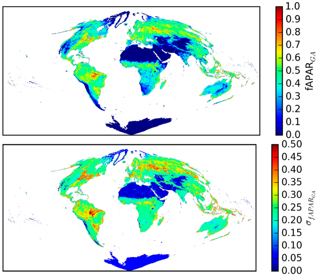
Figure 1.
(Top): global 25 km map of GlobAlbedo-derived fAPAR for DOY 185 2002; (Bottom): uncertainty σfAPAR of retrieved fAPAR for the same time period.
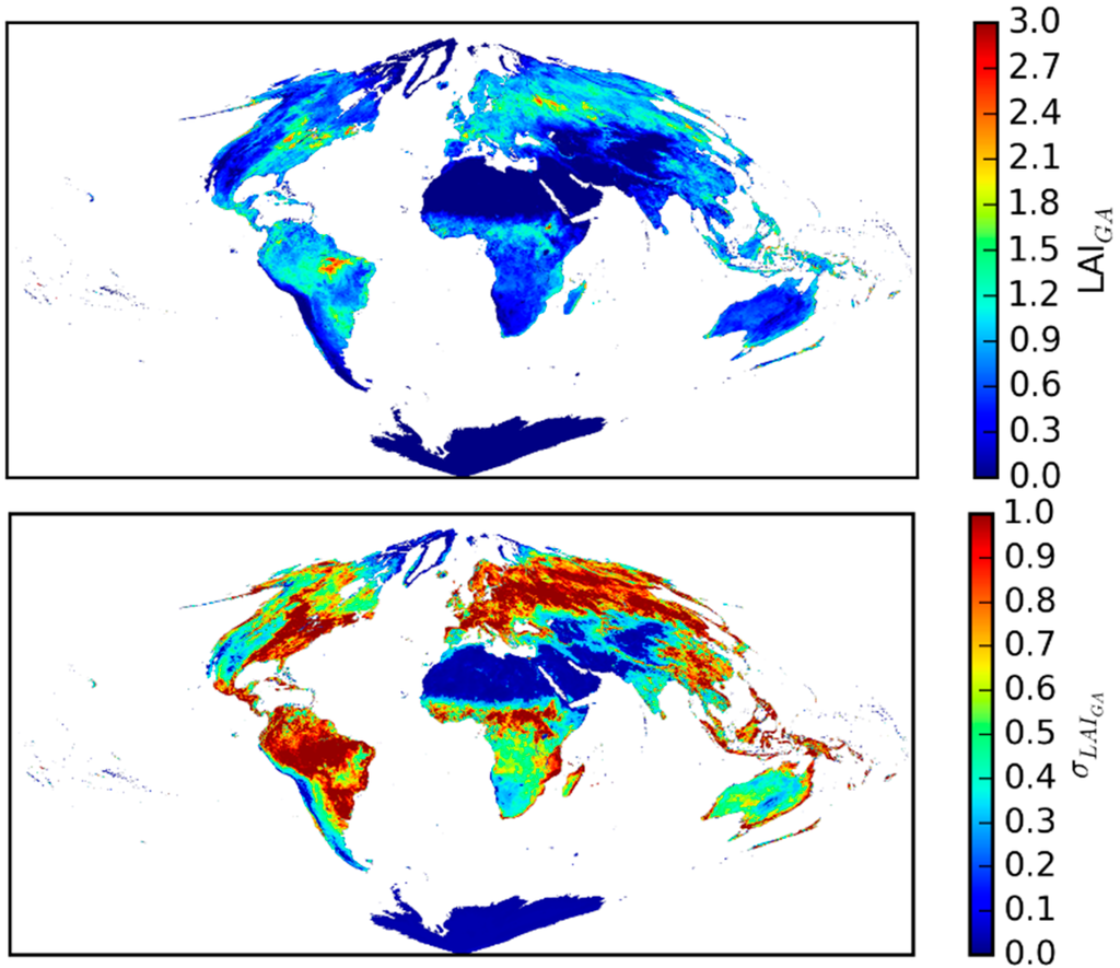
Figure 2.
(Top): global 25 km map of GlobAlbedo-derived LAI for DOY 185 2002; (Bottom): uncertainty σLAI of retrieved LAI for the same time period.
The fAPAR and (effective) LAI values shown above display similar spatial patterns (unsurprisingly) i.e., high fAPAR values co-occur in general with high LAI values, albeit more evenly distributed globally in terms of mean and maximum values. LAI reaches a maximum of around 3 in parts of the US Midwest, Amazonia and Siberia, with the greening of the boreal regions being quite obvious. The uncertainty in fAPAR, σfAPAR, lies mainly between 0.1 and 0.4; uncertainty in LAI, σLAI, is generally highest in areas of high LAI, with some exceptions in Western Europe, China and SE Asia. In these regions, persistent cloud likely causes the higher retrieval uncertainty. This ability of the two-stream inversion package, JRC-TIP, to provide parameter retrieval uncertainty as a consistent part of the retrieval process is a key reason for using such an approach. Data assimilation applications for example, require explicit consideration of uncertainty in driving observations [41,42,43]. The GlobAlbedo product includes uncertainty estimates on a per pixel basis. This is a key difference from other global EO-derived estimates of fAPAR and LAI, for which parameter retrieval uncertainty is either absent, or quantised and hard to interpret as a “real” uncertainty [44].
3.2. Site-Specific and Regional GlobAlbedo-Derived fAPAR and LAI
Site and region comparisons between the GlobAlbedo-derived and MODIS fAPAR and LAI products are presented below, to explore the issue of temporal and spatial consistency between the products, as well as to identify differences. As described above, MODIS fAPAR and LAI estimates are derived using different assumptions from those in the GlobAlbedo JRC-TIP. A key difference is the fact that the MODIS products use a biome-specific 3D solution of radiative transfer in the vegetation canopy [7,8]. Partitioning of the MODIS RT model-based fAPAR and LAI retrievals by biome (corresponding to IGBP land cover classes) allows the canopy type and structure to be considered in the retrieval process explicitly, as well as total % vegetation cover and canopy depth. The MODIS fAPAR/LAI retrieval process is further constrained by biome-specific consideration of clumping, layering (i.e., understory, overstory) and soil background. These constraints introduce fundamental differences between the GlobAlbedo-derived and MODIS products that are likely to be more significant at some times of year and location, than others. Examples of these constraints are the requirement for forest cover to exceed 70% to be considered “forest” in the MODIS retrievals, regardless of type, or the use of snow background at certain times of year and location. In the GlobAlbedo-derived products, the use of a prior based on a surface albedo climatology, allows the albedo retrieval to minimize the impact of outlier (snow, cloud) observations.
Here, we show comparisons between the two datasets over the period 2002–2011 to explore the impacts of these different assumptions, in terms of why and where differences occur. We highlight areas of spatial and temporal consistency (or not as the case may be). We show comparisons at FLUXNET flux tower sites, selected to represent key (wide global coverage) vegetation cover types, namely: grasslands, crops/natural, deciduous broadleaf, evergreen needleleaf, mixed forest, as well as some miscellaneous sites in tropical and temperate regions. We then show regional comparisons over four 1200 × 1200 km tiles, from W. Europe, N. America, Australia and Africa. Finally, we show whole-hemisphere seasonal comparisons.
For the GlobAlbedo-derived parameter values we show the quantified uncertainty arising from the parameter retrieval; for the MODIS values, this is not so clear due to uncertainty being somewhat arbitrarily defined from the RT model assumptions, and so here we simply plot the standard deviation of the spatial average of the 3 × 3 pixels surrounding the flux tower in each case.
3.2.1. Flux Site Comparisons by Cover Type
Locations and cover type descriptions for the FLUXNET site-level comparisons are given above in Section 2.1.6. For each of the selected cover types and for each site, fAPAR and LAI values derived from GlobAlbedo (denoted GA) and MODIS (denoted MO), are compared over the period 2002–2011. Scatter plots of the parameters are then presented, with r2 and RMSE of the linear fit in each case.
Grasslands
The comparisons between GlobAlbedo-derived (GA) and MODIS (MO) values for the grassland sites are shown in Figure 3. For the AU-Stp and US-AR2 sites the fAPAR values agree closely in terms of peak magnitude and timing albeit with the GA values lying slightly above the MO values during peak (summer) times. In the case of the AU-Stp site, the GA values show a longer delay before senescence in most years. This is also apparent in the RU-Upo site. Peak GA fAPAR values are lower than their MO counterparts for the CN-Du3 and RU-Upo sites. Agreement is reflected in the r2 values, which range from 0.76 to 0.95. GA-derived values lie below the corresponding MO values for all sites bar US-Ar2 i.e., there is a positive slope between GA and MO values. The intercept between the two estimates of fAPAR is ≤ 0.12 in all cases.
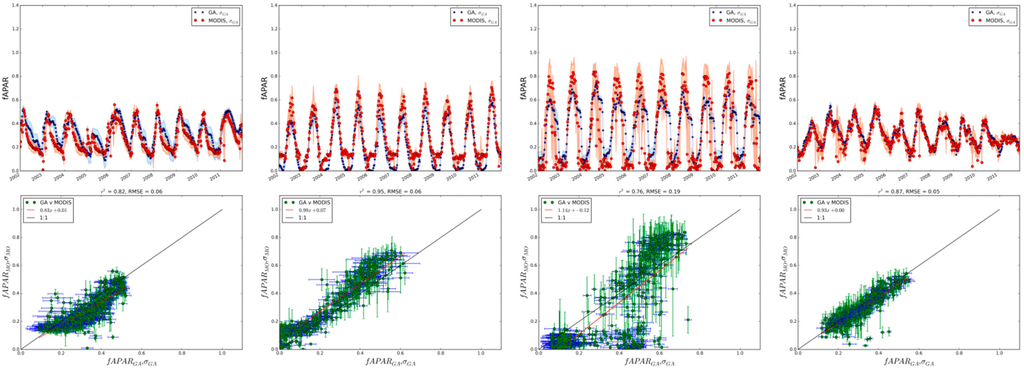
Figure 3.
Top row: GlobAlbedo-derived and MODIS fAPAR values for 2002–2011; second row: scatter plot of fAPAR values; third row: GlobAlbedo-derived and MODIS LAI values for 2002–2011; fourth row: scatter plot of LAI values. Error bars for GlobAlbedo values represent the uncertainty of parameter retrieval, and for the MODIS data, the variance of the 3 × 3 pixel window centered on the comparison site.
The LAI values lie between 1 and 2 for all sites bar RU-Upo, where peak values approach 4 in the summer. The timing of greenup agrees within 8–16 days between the two sets of products, and within 16 days for senescence. This suggests that estimates of canopy phenology properties will be consistent between the two datasets for this cover type. r2 values between the two LAI datasets lie between 0.77 and 0.87 with the exception of CN-Du3, which has a larger slope of ~2 and intercept of 1.3. This suggests there is a particular difference at this site, in terms of canopy structure between the datasets. Other than this there is a consistent positive slope i.e., as for fAPAR, MODIS LAI values are generally higher than the corresponding GA-derived values. The variation in uncertainty is apparent in both fAPAR and LAI, particularly at the RU-Upo and US-AR2 sites.
Deciduous Broadleaf Forest
The comparisons between GlobAlbedo-derived (GA) and MODIS (MO) values at the deciduous broadleaf forest sites are shown in Figure 4. There is a wider disagreement between the GA and MODIS fAPAR values in terms of peak values than for the grasslands sites, with the GA values consistently lower at the summer peak for all sites. Conversely, the GA values tend not to reach 0 in the winter, falling to 0.01–0.02, whereas the MO values tend to be lower and even 0 in some cases. In the case of the AU-Stp site, the GA values show a longer delay before senescence in most years. The timing of greenup and senescence agree within 8–16 days for all sites. The uncertainty in both datasets is also larger than for the grassland sites above, at both summer peak values, but also in winter. In the latter case this is likely to be due to clouds, snow and low sun angles, hence poor sampling and poor quality observations in general. r2 values for fAPAR range from 0.86 to 0.92, with positive slope between 1.34 and 1.43 and intercept between 0.07 and 0.11.
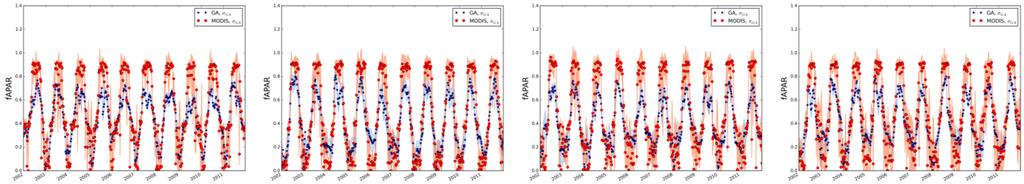
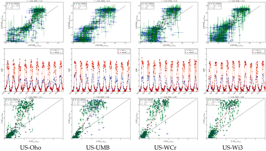
Figure 4.
Top row: GlobAlbedo-derived and MODIS fAPAR values for 2002–2011; second row: scatter plot of fAPAR values; third row: GlobAlbedo-derived and MODIS LAI values for 2002–2011; fourth row: scatter plot of LAI values. Error bars for GlobAlbedo values represent the uncertainty of parameter retrieval, and for the MODIS data, the variance of the 3 × 3 pixel window centered on the comparison site.
The LAI values in this case highlight the difference between the two datasets, with the MO values being substantially higher in all peak times, by a factor of two in some cases. The r2 values lie between 0.84 and 0.90, with slope of around 2–2.3 in all cases, and with intercepts between −0.3 and −0.2.
Evergreen Needleleaf Forest
The comparisons between GlobAlbedo-derived (GA) and MODIS (MO) values at the evergreen needleleaf forest sites are shown in Figure 5. There is a much greater disagreement between the GA and MODIS fAPAR values than in previous cases. This difference is apparent across all sites, with peak MO values being approximately double the GA values in all cases. Timing is also somewhat different between the two estimates, particularly for the US-NR2 site, where both greenup and senescence are delayed in the MODIS fAPAR compared to the GlobAlbedo-derived values, by up to 2–3 weeks in some cases. The uncertainty in both datasets is also large, but particularly for the MODIS at the DE-SfN and FI-Ves sites. This is almost certainly due to clouds, snow and low sun angles, particularly in the Finnish site. For fAPAR, r2 values range from 0.52 to 0.77, i.e., markedly lower than for the cover types above, with positive slope ranging from 1.4 up to 2.23 for the FI-Ves site, and intercept between −0.16 and 0.1.
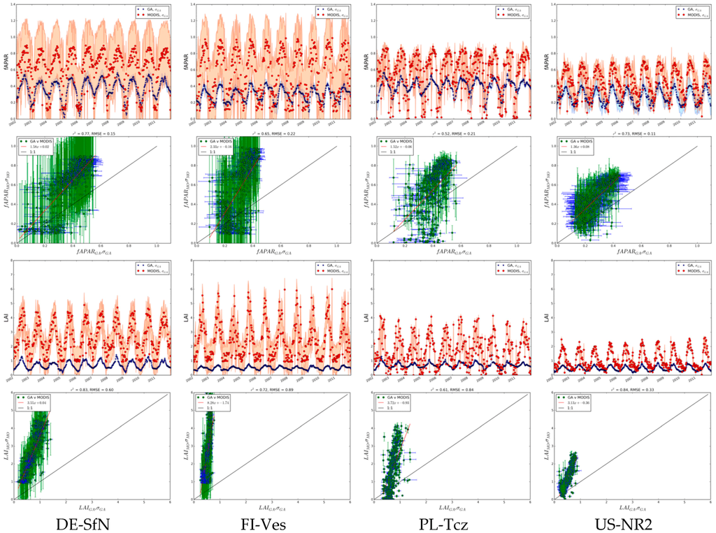
Figure 5.
Top row: GlobAlbedo-derived and MODIS fAPAR values for 2002–2011; second row: scatter plot of fAPAR values; third row: GlobAlbedo-derived and MODIS LAI values for 2002–2011; fourth row: scatter plot of LAI values. Error bars for GlobAlbedo values represent the uncertainty of parameter retrieval, and for the MODIS data, the variance of the 3 × 3 pixel window centered on the comparison site.
The LAI values agree in timing, but not in magnitude at all. This is illustrated by r2 values of 0.6–0.84, but with very large slopees in all cases, from 3.1 to >8 in the case of the FI-Ves site, and intercept values of −1.74–0.04. These values would suggest that there is a significant difference in the way the respective parameter retrievals operate over evergreen needleleaf forests. The MODIS algorithm requires tree cover to exceed 70% to be classified as forest, which may be marginal in some of these areas; it is also possible that including understory in the MODIS RT retrieval scheme introduces further differences. Notably, uncertainty is large in the MODIS LAI retrievals, particularly in the DE-SfN and FI-Ves sites. The latter is a very northerly site, with a short growing season, persistent snow cover and observations that will contain low sun angles through large parts of even mid-summer. These factors will all introduce greater uncertainty to RT parameter retrievals.
Mixed Forest
The comparisons between GlobAlbedo-derived (GA) and MODIS (MO) values at the mixed forest sites are shown in Figure 6. The ST-StM and CH-Dsc sites show similar behavior in fAPAR to the evergreen needleleaf forest sites above i.e., with peak MO values being ~1.5× higher than GA. Lower values agree well, and the timing of greenup/senescence is generally within 2 weeks in the two datasets. The exception to this is the US-Ha2 site, where peak values are closer, but timing is more variable. The r2 values lie between 0.77 and 0.88 with slope lying between 1.1 and 1.74, and with intercept −0.1–0.08.
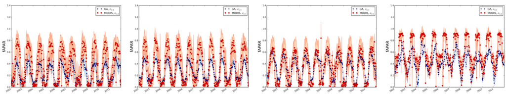
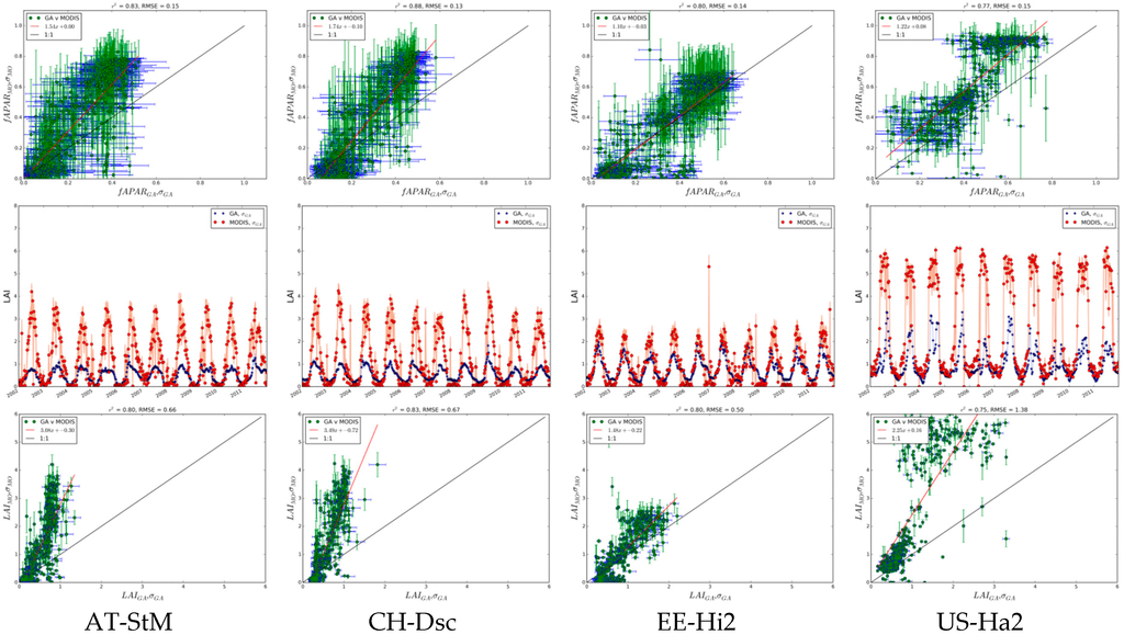
Figure 6.
Top row: GlobAlbedo-derived and MODIS fAPAR values for 2002–2011; second row: scatter plot of fAPAR values; third row: GlobAlbedo-derived and MODIS LAI values for 2002–2011; fourth row: scatter plot of LAI values. Error bars for GlobAlbedo values represent the uncertainty of parameter retrieval, and for the MODIS data, the variance of the 3 × 3 pixel window centered on the comparison site.
The closer agreement in timing is illustrated by the LAI values, albeit with large differences in peak values for the AT-StM, CH-Dsc and US-Ha2 cases particularly. The r2 values lie between 0.75 and 0.83, with slope between 1.5 and 3.5 and intercept between −0.72 and 0.2
Crop/Natural
The comparisons between GlobAlbedo-derived (GA) and MODIS (MO) values at the mixed forest sites are shown in Figure 7. In these cases, the fAPAR values agree closely in both timing and peak values for all sites. The African site, ML-Kem, shows a different phenology between the two datasets, with a much more gradual senescence in the MO values than in the GA values. Again, this may be a result of the explicit consideration of understory vegetation in the MODIS values, which is typically strongly dependent on seasonal rainfall. The otherwise close agreement in timing and peak values is demonstrated by the r2 values of 0.81–0.95, with much lower slope (0.97–1.42) than for the forest sites above and intercepts in the range −0.2–0.1.
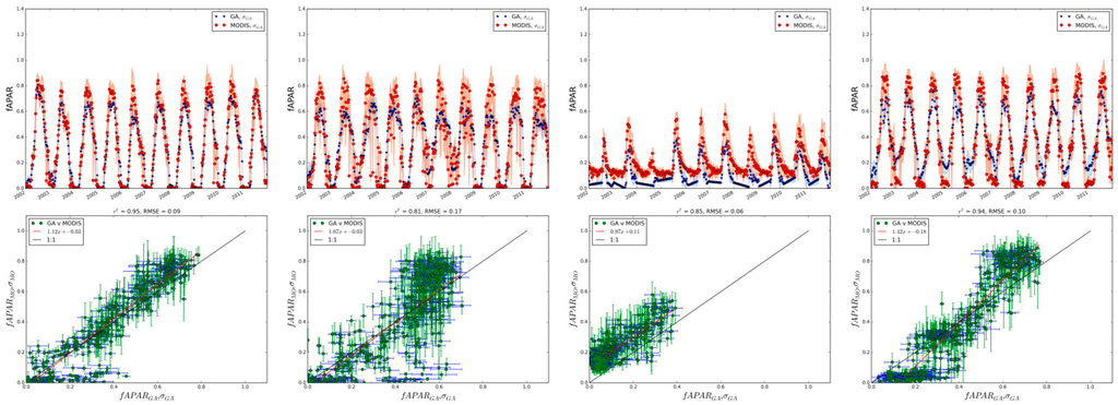
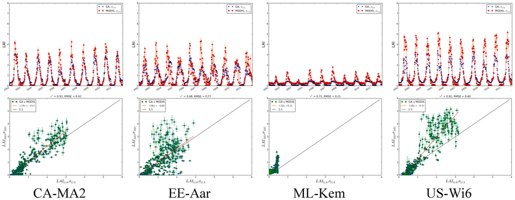
Figure 7.
Top row: GlobAlbedo-derived and MODIS fAPAR values for 2002–2011; second row: scatter plot of fAPAR values; third row: GlobAlbedo-derived and MODIS LAI values for 2002–2011; fourth row: scatter plot of LAI values. Error bars for GlobAlbedo values represent the uncertainty of parameter retrieval, and for the MODIS data, the variance of the 3 × 3 pixel window centered on the comparison site.
LAI values agree to within 10%–15% in peak season for CA-MA2 for example. Agreement on timing is also strong for CA-MA2 and US-Wi6, as demonstrated by r2 values > 0.9, but lower for EE-Aar and ML-Kem (r2 values 0.68 and 0.71 respectively). Slope in these sites lies between 1.06 and 1.32 (again, the ML-Kem site is the higher one) and intercepts are −0.41–0.15.
Miscellaneous
The comparisons between GlobAlbedo-derived (GA) and MODIS (MO) values at the miscellaneous sites are shown in Figure 8. The fAPAR values in the European sites (unsurprisingly) follow very similar patterns to the evergreen needleleaf and mixed forest sites above, with close timing (r2 ~ 0.6), but very different peak values between GA and MO values. Both these sites experience significant and extended snow cover during the winter, which will affect retrieval values and timing during spring particularly. In addition, both sites have significant understory which may have a different phenology to the overstory forest canopy. Mixed phenology of this sort is always likely to introduce uncertainty in retrieved timing information. This is also likely to affect the MODIS and GlobAlbedo-derived parameter retrievals slightly differently due to the different assumptions underlying the retrieval methods.
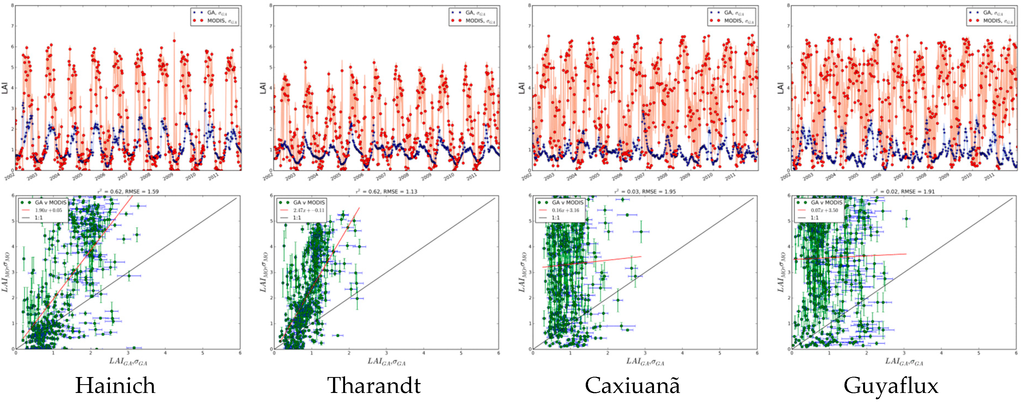
Figure 8.
Top row: GlobAlbedo-derived and MODIS fAPAR values for 2002–2011; second row: scatter plot of fAPAR values; third row: GlobAlbedo-derived and MODIS LAI values for 2002–2011; fourth row: scatter plot of LAI values. Error bars for GlobAlbedo values represent the uncertainty of parameter retrieval, and for the MODIS data, the variance of the 3 × 3 pixel window centered on the comparison site.
In the two tropical sites fAPAR values are particularly variable, for both the GA and MO data, and with a much less obvious (or clear) seasonality (r2 ~ 0.1). This is likely to be due to both cloud, and the inherently different seasonality in these tropical regions, dominated by evergreen broadleaf trees and rainfall seasonality. The uncertainty in the MODIS values is testament to this variability.
The LAI values are very different between GA and MO across all sites, but with almost no correlation in the tropical sites. This is reflected in r2 values close to 0. This would indicate that the derived values should be interpreted with care in terms of timing and magnitude (relative or otherwise) at sites of this sort.
Summary of Site Comparisons
A summary of the results for the various sites is presented in Table 2 below, comprising the upper and lower values of the slope and intercept of the linear regression between the GlobAlbedo-derived and MODIS values of fAPAR and LAI.
Table 2.
Summary of bias (slope) and intercept of comparisons for all biome types.
3.2.2. Regional Comparisons
Comparisons are presented across complete 1200 × 1200 km tiles, covering some of the regions outlined above in the site-level comparisons. MODIS and GlobAlbedo-derived fAPAR and LAI values are compared for the following tiles specified by the horizontal and vertical MODIS tile IDs from the MODIS tile map [32]:
- h09v05: Central USA
- h18v03: Western Europe
- h18v07: Central West Africa
- h29v12: South Australia
Tiles are compared from a given 8-day period in 2002 at mid-summer for each tile i.e. day of year (DOY) 185 for northern hemisphere tiles h09v05, h18v03, h18v07, and DOY 001 for southern hemisphere tile h29v12. In each case, scatter plots of the GlobAlbedo-derived and MODIS fAPAR and LAI values for all pixels in each tile, for all equivalent DOY values over the period 2002–2011 are also shown. These scatter plots are shown as 2D histograms (or “heatmaps”) i.e., the (x, y) location of each point represents the value of GlobAlbedo-derived and MODIS parameter in 20 bins along each axis respectively, and the color represents the frequency of samples in each bin. Comparisons are shown first for fAPAR and then LAI for each of the tiles. Agreement across tiles ought to be expected to be lower than for individual sites, due to the mixed nature of the cover types covered in a given tile. This is particularly true for very heterogeneous tiles where there is significant agriculture i.e., tile h18v03 for W. Europe. These comparisons are included to illustrate large-scale regional trends between the two datasets.
Central USA: Tile h09v05
Figure 9 shows the comparison between GlobAlbedo and MODIS fAPAR and LAI values for 2002 DOY 185 over central Southern USA. In this case, significant cloud cover over the region means that both coverage and retrieval quality are variable. The vegetation is primarily sparse grassland, scrub, savanna and low-cover woodland, with correspondingly low retrieved LAI values over much of the tile except in the SE corner. This results in low fAPAR values over much of the tile. The correlation between the GlobAlbedo-derived and MODIS fAPAR values shows r2 = 0.3, and for LAI r2 = 0.08 i.e., there is very little spatial correspondence between the GA and MO values, particularly for LAI. There is clearly a strong seasonal variation in LAI, with much higher values (and range) observed over DOY 185 than for DOY 361 over both years. Areas of low vegetation cover such as this (and/or particularly heterogeneous areas) are likely to prove more problematic for RT parameter retrieval at these scales than mid-range LAI, heterogeneous regions. Correct identification of the underlying land cover class (or biome) is simply more difficult/uncertain, resulting in potentially higher uncertainty in retrieved RT model parameters. This is particularly the case for scrub/grasslands and low LAI savannas.
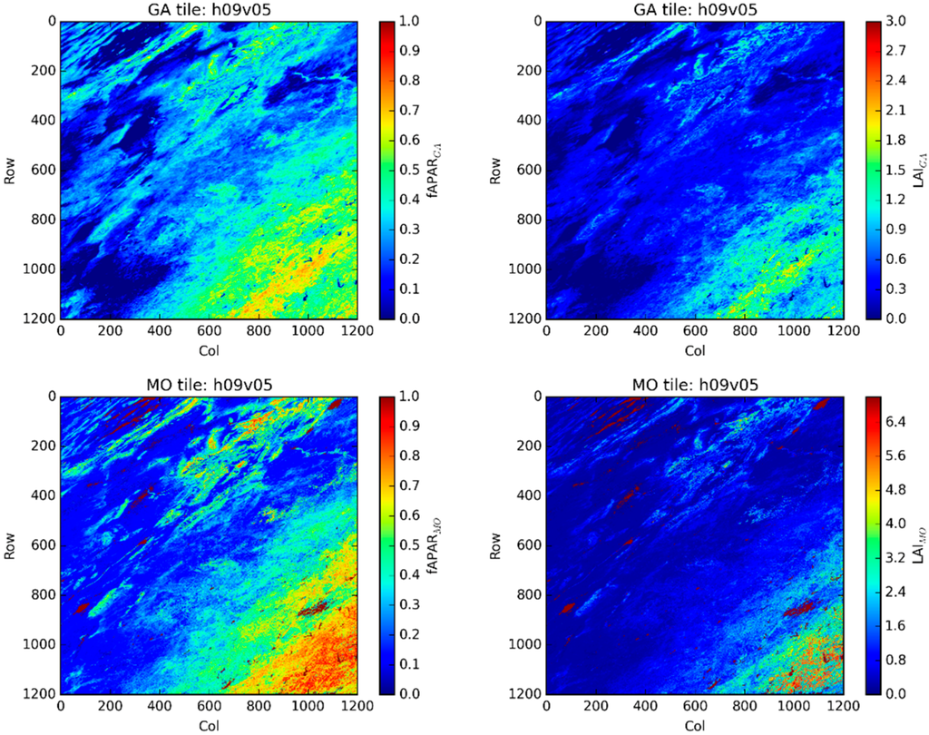
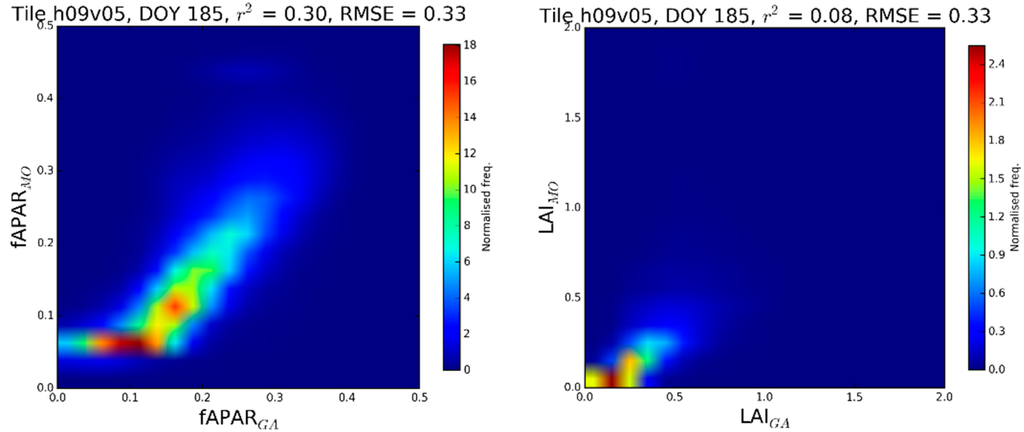
Figure 9.
Regional comparison of GlobAlbedo-derived (GA) and MODIS (MO) fAPAR and LAI. (Top row): GA fAPAR (left panel) and LAI (right panel); (middle row): MO fAPAR (left panel) and LAI (right panel); (bottom row): heatmap scatter plot between the GA (x-axis) and MO (y-axis) values, DOY 185 for all years 2002–2011: fAPAR (left panel) and LAI (right panel).
Western Europe: Tile h18v03
Figure 10 shows the comparison between GlobAlbedo-derived and MODIS fAPAR and LAI values for 2002 over Western Europe (note that the fill values over ocean are 0 for GlobAlbedo and 1 for MODIS). Firstly, in terms of annual trends, we see the expected high values of LAI and fAPAR in the middle of the year, due to the large amount of crop coverage in the tile. In addition, apparent is the heterogeneous nature of the land cover, particularly in the southern and western parts. Peak values are consistent between years, although the values for 2006 are lower than in 2005. Agreement between the GlobAlbedo-derived and MODIS fAPAR and LAI values is much higher than for the tile above, with r2 values of 0.8 and 0.77 for fAPAR and LAI respectively. The consistently lower values of both GlobAlbedo-derived LAI and fAPAR (and much lower range) discussed above, are also apparent in the 2D scatter plots.
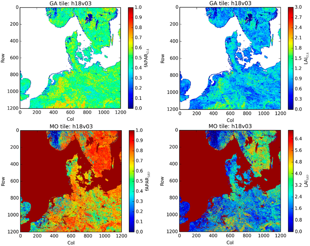
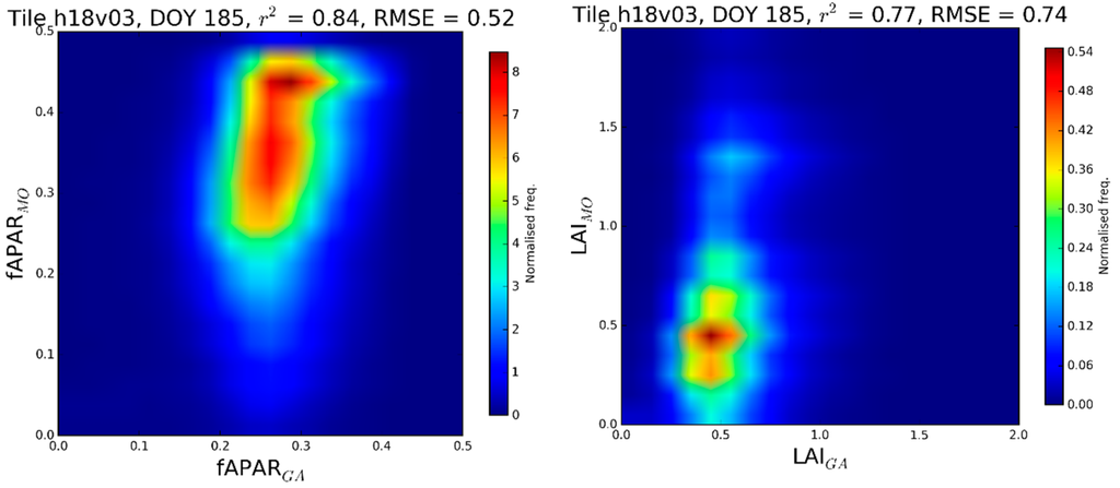
Figure 10.
Regional comparison of GlobAlbedo-derived (GA) and MODIS (MO) fAPAR and LAI. (Top row): GA fAPAR (left panel) and LAI (right panel); (middle row): MO fAPAR (left panel) and LAI (right panel); (bottom row): heatmap scatter plot between the GA (x-axis) and MO (y-axis) values, DOY 185 for all years 2002–2011: fAPAR (left panel) and LAI (right panel).
Central and West Africa: Tile h18v07
Figure 11 shows the comparison between GlobAlbedo-derived and MODIS fAPAR and LAI values for DOY 185 in 2002 over Central and West Africa. As above for the US tile, cloud is clearly an issue during this period. The fAPAR and LAI values are generally low in both cases, indicating the sparse grassland and savanna vegetation cover. Correlation between GlobAlbedo-derived and MODIS LAI is negative for this tile/date, with r2 ~ 0.5. As explained above for the Caxiuanã and Guyaflux tower site comparisons, this may be due to strong spatial and temporal patterns of seasonal rainfall variation across the tile. The response of grasslands, and savanna more generally, is very dependent on (and even defined by) rainfall. This is likely to dominate vegetation timing patterns in these areas, making comparisons difficult. The implication is that care should be taken in interpreting the values from either dataset in this sort of area: timing and magnitude of fAPAR or LAI will be dependent on which sort of retrieval is used.
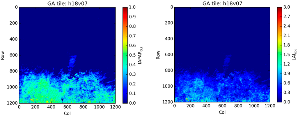
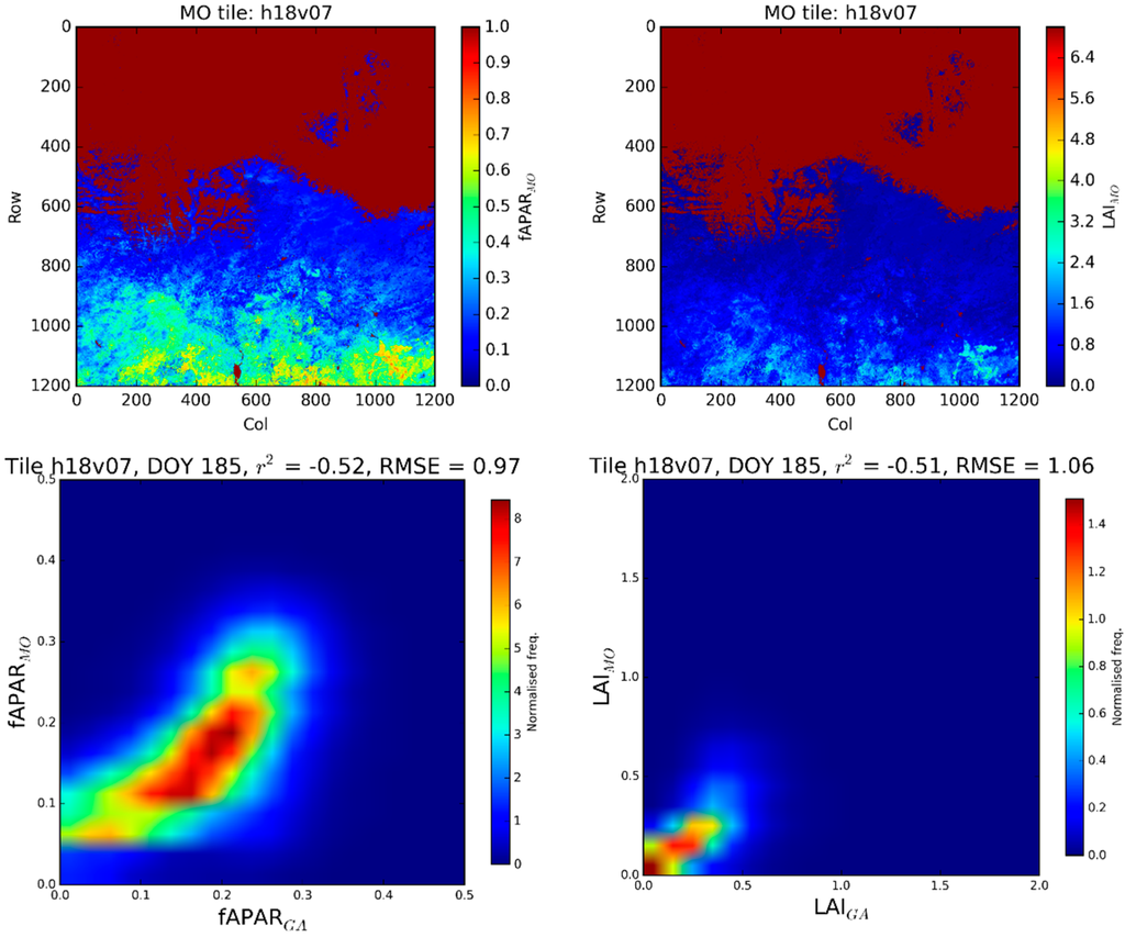
Figure 11.
Regional comparison of GlobAlbedo-derived (GA) and MODIS (MO) fAPAR and LAI. (Top row): GA fAPAR (left panel) and LAI (right panel); (middle row): MO fAPAR (left panel) and LAI (right panel); (bottom row): heatmap scatter plot between the GA (x-axis) and MO (y-axis) values, DOY 185 for all years 2002–2011: fAPAR (left panel) and LAI (right panel).
South Australia: Tile h29v12
Figure 12 shows a comparison between GlobAlbedo-derived and MODIS fAPAR and LAI values for DOY 001 2202 over Southern Australia. fAPAR values are much higher across the SE coastal region, where much of the vegetation in the tile is located. The interior regions have very low vegetation cover, reflected in the low fAPAR and LAI values across much of these areas. LAI values across this region are correspondingly low for both datasets (compared with tile h18v03 above), but with some spatial consistency—particularly the higher values across the SE coast. The S. Hemisphere location might suggest that seasonal variation should be reversed compared with N. Hemisphere regions i.e., high early in the year, low at the start/end. However, given the small variation in general across the tile, there is far less seasonal variation than for tile h18v03. There is a much stronger agreement between the GlobAlbedo-derived and MODIS values at this site, indicative of a more homogeneous cover type. The correlation of fAPAR and LAI shows r2 > 0.9 for both. This indicates that although the LAI values are consistently low, a much stronger agreement between GlobAlbedo-derived and MODIS values exists for this kind of cover than for the others shown above. In these regions it is entirely appropriate to compare and even cross-calibrate GlobAlbedo-derived and MODIS values.
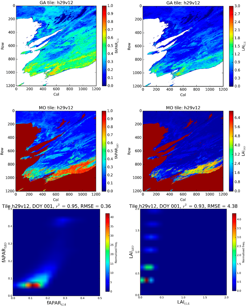
Figure 12.
Regional comparison of GlobAlbedo-derived (GA) and MODIS (MO) fAPAR and LAI. (Top row): GA fAPAR (left panel) and LAI (right panel); (middle row): MO fAPAR (left panel) and LAI (right panel); (bottom row): heatmap scatter plot between the GA (x-axis) and MO (y-axis) values, DOY 001 for all years 2002–2011: fAPAR (left panel) and LAI (right panel).
3.3. Whole-Hemisphere Comparisons
Comparisons are shown between the GlobAlbedo-derived (GA) and MODIS (MO) fAPAR and LAI values, on a hemisphere and seasonal basis, for 2005 and 2011 (towards the start and end of the GA record) in Figure 13 (fAPAR) and Figure 14 (LAI). All valid land tiles lying in horizontal rows 0–8 on the MODIS tile map are considered as Northern Hemisphere (NH, 161 tiles); all valid land tiles lying in horizontal rows >8 are considered Southern Hemisphere (SH, 113 tiles). Data from DOY 185 (NH) and DOY 361 (SH) are considered “summer”; data from DOY 001 (NH) and DOY 185 (SH) are considered “winter”. Each tile in each summer/winter case, for each year, is compared by calculating a linear regression between the GA-derived and MO values, for all valid land pixels. The resulting differences between the two are characterized by the slope and intercept of the regression in each case, and the RMSE of the linear model fit, weighted by the number of valid pixels in each tile. These values are collected and shown in (normalised) histograms below. These histograms indicate the consistency (or otherwise) of the agreement between the GA-derived and MO values from season to season and from year to year. They also summarize the overall magnitude of slope and intercept between the GA-derived and MO values.
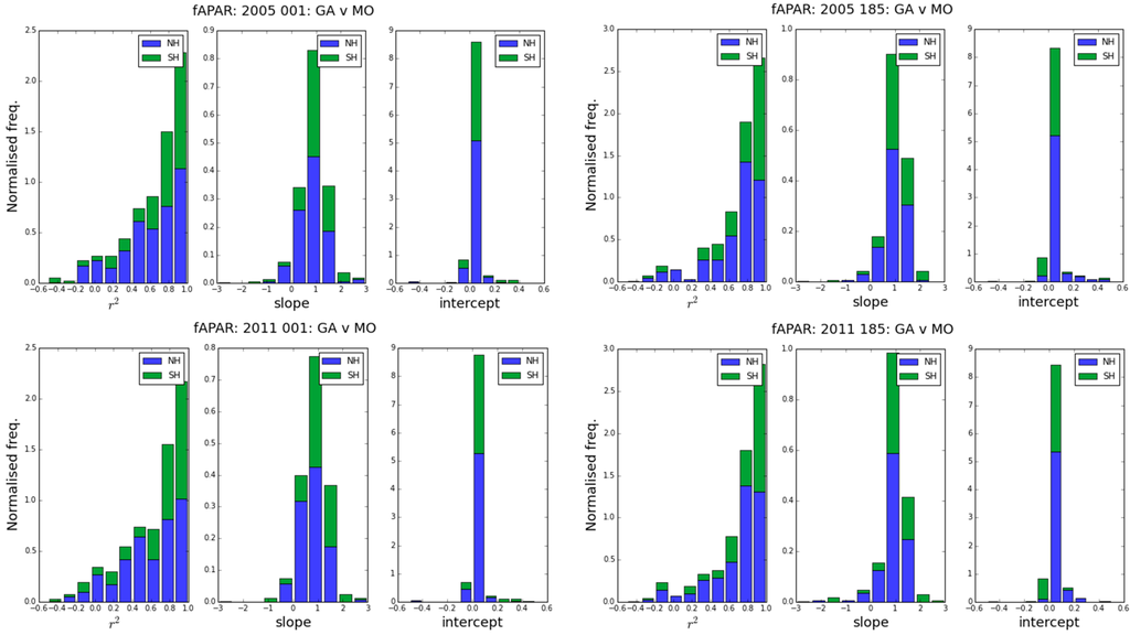
Figure 13.
Comparison of whole hemisphere GlobAlbedo-derived (GA) and MODIS (MO) fAPAR. Each panel shows a histogram of NH and SH histograms of correlation coefficient (r2), slope and intercept, for regression of GA v MO. (Top row), 2005: (left panel): day-of-year (DOY) 001; (right panel): DOY 185. (Bottom row), 2011: (left panel): DOY 001; (right panel): DOY 185.
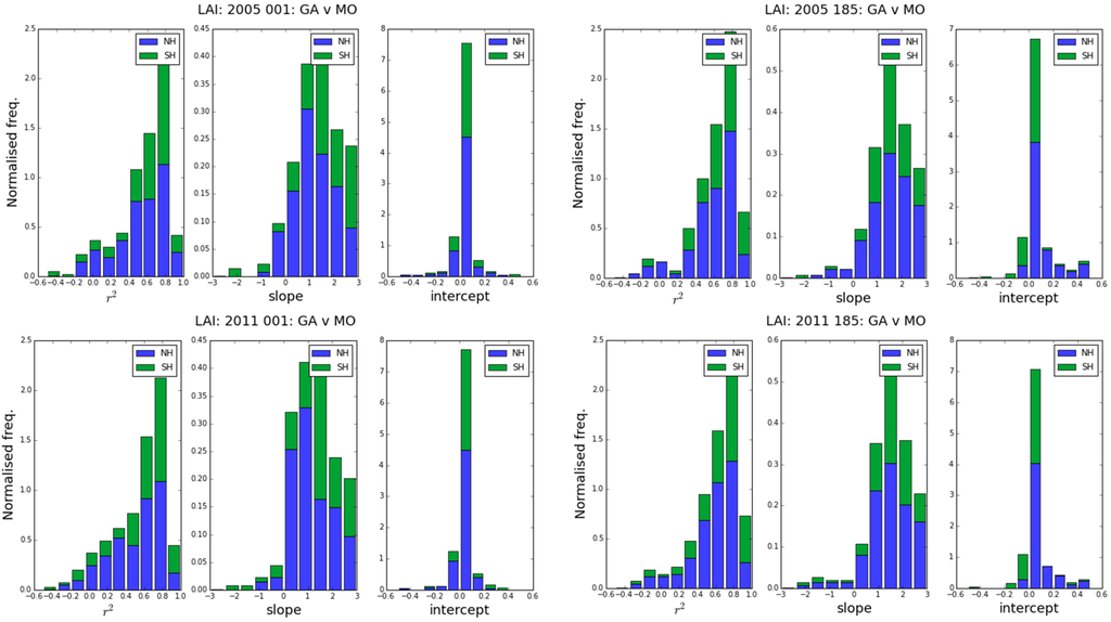
Figure 14.
Comparison of whole hemisphere GlobAlbedo-derived (GA) and MODIS (MO) LAI. Each panel shows a histogram of NH and SH correlation coefficient (r2), slope and intercept, for regression of GA v MO. (Top row), 2005: (left panel): day-of-year (DOY) 001; (right panel): DOY 185. (Bottom row), 2011: (left panel): DOY 001; (right panel): DOY 185.
Figure 13 demonstrates correlation between the fAPAR products is almost exclusively positive with r2 values exceeding 0.8 for: 37% of NH tiles and 52% of SH tiles on 2005 DOY 001 (NH winter, SH summer). This fraction rises in 2005 for DOY 185 to 48% and 63% of the NH and SH tiles respectively. For 2011, the distribution of r2 values is almost identical. The slope and intercept of the correlation between the two products obviously represent the translation from one to the other. If the two datasets are to be compared or used in conjunction with each other, then these values could be used for transforming from one to the other. From Figure 13 the gradient between the fAPAR products lies between 0.5 and 1.5 for ~70% of all tiles on DOY 001, and 80% of all tiles on DOY 185 for both 2005 and 2011. Lastly, the intercept of the linear regression of the fAPAR products lies within −0.1 and 0.1 for 90%–95% of all tiles in both 2005 and 2011, with a slightly greater spread of values for winter cases than summer.
The correlation between LAI estimates summarized in Figure 14 is slightly weaker than for fAPAR, with r2 exceeding 0.8 for 13% (NH) and 20% (SH) of tiles for 2005 DOY 001, and 15% (NH) and 34% (SH) of tiles for 2005 DOY 185. The values for 2011 are very similar. This indicates that the correlation is stronger in general for the SH tiles. The gradient of the correlation between the LAI products lies between 0.5 and 1.5 for 42% (NH) and 24% (SH) of cases in 2005 DOY 001. These percentages switch around for 2005 DOY 185, to 27% (NH) and 34% (SH). This suggests there is a greater variation in the gradient of the relationship between the LAI estimates in winter than in summer. For 2011, the gradient lies between 0.5 and 1.5 for 31%–38% of all cases.
Finally, the LAI regression intercept lies within −0.1 and 0.1 for ~80% of cases for all NH and SH tiles in 2005 DOY 001. For 2005 DOY 185 this percentage drops to 62% of NH tiles but remains high at 86% for the SH tiles. For 2011, the behavior is very similar—high values for all SH cases, but falling between NH winter and summer.
4. Discussion
Values of LAI and fAPAR derived from the JRC-TIP algorithm applied to the GlobAlbedo data were compared with MODIS-derived LAI and fAPAR estimates. As noted previously, these two sets of products are based on different assumptions: the GlobAlbedo-derived fAPAR and LAI are generated using a 1D RT model inversion scheme designed to be consistent with the observations used to drive it; the MODIS products are generated using a 3D RT model scheme. As a result the LAI values are “real” in the sense that they represent the LAI within this 3D scheme, assuming some biome-specific cover, clumping and understory/soil properties. However, the MODIS LAI values are still not real in as much as they depend on these biome-specific assumptions, are derived from large-scale (250 m to 1 km) observations assuming cover is homogeneous within each pixel, and assume the underlying biome map is accurate at this scale. All of these issues combine to make the resulting LAI (and corresponding fAPAR) values essentially impossible to verify in any real sense.
The JRC-TIP GlobAlbedo approach results in values of LAI (and derived fAPAR) that are consistent with the 1D approximation to a 3D RT problem, where clumping is not accounted for, but not intended to correspond to the real LAI and fAPAR of the surface. This approach is useful for the following reasons: (i) consistency between RT model assumptions and observations is ensured; (ii) meaningful uncertainty core to the GlobAlbedo approach and is provided with the derived LAI and fAPAR values; (iii) the inversion scheme can be applied globally, without any requirement for any biome-specific structural (cover, clumping, understory) assumptions required for 3D RT model approaches; and (iv) the RT scheme is very similar to schemes used by many Earth System Models (ESMs) [22]. However [43] note that even 1D RT schemes used in ESMs are often implemented differently, leading to differences in both fAPAR (and hence photosynthesis) and surface albedo.
A key point to note in the comparison between GlobAlbedo and MODIS products above is the temporal consistency across each year. At a given site, and even averaged over several pixels, the temporal variation of the MODIS values can be up to a factor of 2 or more at times between subsequent estimates (see Figure 3, Figure 4, Figure 5, Figure 6, Figure 7 and Figure 8). We note that this variation has reduced significantly between collections 5 and 6 of MODIS LAI/fAPAR: previous sample-to-sample variation could be 7× or more (see [44] for summary of changes from collection 5 to 6). This temporal variation is largely due to the influence of residual cloud and snow contamination that causes poor quality RT model retrievals, even though they may not be flagged as such in the underlying reflectance data. Additional improvements made in collection 5 to collection 6 of the MODIS LAI/fAPAR retrievals include an updated underlying land cover map. This will potentially affect retrieved parameter values by altering the biome type used in RT model retrieval. This is likely to be of most importance in areas with relatively low (and mixed) vegetation cover, such as semi-arid regions, savannas and scrub grassland [45,46]. These regions may also have rapidly changing phenology, which can introduce further uncertainty in RT model retrievals based on land cover classifications that may be static or updated relatively infrequently (annually or less) [47]. The authors of [48] showed that fAPAR from MODIS and SPOT-VGT are particularly variable in woody savanna regions, due to the combination of low vegetation cover, mixed woody cover and dynamic phenology. The authors of [47] looked explicitly at the issue of mixed cover and biome misclassification on uncertainty in retrieved MODIS LAI and showed that this was most important in savannas, resulting in uncertainty in retrieved LAI of up to 0.51. The GlobAlbedo albedo values are based on a moving window approach which generates a model-based prediction of albedo with a prior expectation [32]. This approach is more robust to outliers, which is apparent in the temporal profiles, and is also likely to provide a more conservative estimate of fluxes than the MODIS data. The GlobAlbedo-derived values are also not constrained by an underlying biome map and so will not be affected by land cover misclassification. This may explain the variability and much lower correlation between the GlobAlbedo- and MODIS derived values seen for tile h09v05 above (central Southern USA, Section “Central USA: Tile h09v05”, Figure 9).
These points aside, the comparisons show that in general timing (phenology) information agrees within one or two weeks, particularly in the most important green-up and senescence phases of the year. This is about as good as might be expected given the various uncertainties introduced by the temporal compositing window of the MODIS data and the assumptions underlying both retrieval methods.
The MODIS values tend to remain high during the winter, particularly for the evergreen needleleaf sites (see Figure 4). If these values were used for driving productivity models, then this would likely lead to over-estimates of winter GPP and NPP. However, the GlobAlbedo-derived values tend to be much lower/more conservative in the peak season, largely due to their being effective values. This would have the reverse effect of depressing estimates of GPP and NPP in the summer. If the LAI and fAPAR are to be used for timing or phenology studies, the clear winter phase of GlobAlbedo-derived LAI and fAPAR is likely to be advantageous.
In general, the different RT model schemes lead to consistently lower values of LAI and fAPAR in the GlobAlbedo-derived products compared with MODIS. This is clearly demonstrated in the values of the slope of the regressions summarized in Table 2, which are almost all >1 for fAPAR, except for one or two cases where the correlations are particularly poor anyway. For LAI, this difference is even more marked with slopes mostly between 1.5 and 3 but up to 8 in one or two cases. It is worth stressing again that a naïve comparison of one product against the other might lead to the conclusion that they are fundamentally incompatible, rather than estimates of the same properties made under different (but equally valid) assumptions. As a result, if values are to be used for surface energy balance, or driving global vegetation models, care must be taken to take this into account when using either product [49,50]. The per-tile comparisons shown in Figure 9, Figure 10, Figure 11 and Figure 12 show the same general behavior i.e., high correlations in areas of seasonal vegetation, less likely to be affected by cloud and/or snow, lower correlations elsewhere, and with consistently lower values of both GlobAlbedo-derived LAI and fAPAR (and much lower range).
The slope and intercepts in the whole hemisphere comparisons, shown in Figure 13 and Figure 14, are quite stable between NH and SH. However, the variation in slope and intercept is larger for winter than summer cases, which reflects the generally lower values of both, and more importantly, the reduced quality and frequency of observations.
Globally, the comparisons between GlobAlbedo and MODIS fAPAR show:
- mean slope 1.01, σ = 0.78
- mean intercept 0.03, σ = 0.10
The corresponding global comparisons between GlobAlbedo and MODIS LAI show:
- mean slope 1.70, σ = 1.73
- mean intercept 0.15, σ = 0.58
The recommendation we would make is that if users require a transformation between GlobAlbedo-derived LAI and fAPAR products against those derived from different RT approaches and assumptions, particularly for a given site, they can calculate a site-based or tile-based local transformation using the GlobAlbedo nearline subsetting tool: [37]. This tool also allows users to obtain corresponding GlobAlbedo albedo values. Our results also suggest that particular care is required when comparing (or using) values over sites with poor observation quality (cloud, snow low sun angles) and/or strong differences in overstory/understory phenology. This is of course likely to be true for other EO-derived estimates of fAPAR and LAI.
5. Conclusions
We have presented a new global 1 km fAPAR and LAI dataset, covering the years 2002–2011, derived from the ESA GlobAlbedo product. It is derived using a 1D radiative transfer (RT) model solution to the problem of RT in an inherently 3D canopy medium. The RT parameter retrieval scheme used to derive fAPAR and LAI is intended to be applied globally with no requirement for an underlying biome map and provides a consistent estimate of the uncertainty in derived parameters. We have compared the resulting GlobAlbedo-derived fAPAR and LAI estimates with the widely-used MODIS estimates of the same properties, over different years, at site, region and hemisphere scale. We show that the products agree closely in most cases in terms of timing, but not in terms of peak values, with the GlobAlbedo-derived values generally lower due to the underlying RT model assumptions, particularly LAI. These differences are strongly dependent on biome type (in the sense of the MODIS scheme) and season. The GlobAlbedo-derived values are consistent with the RT schemes of large-scale Earth system models, but less so with finer-scale ground-based (indirect) estimates of fAPAR and LAI. We provide an estimate of the coefficients required to calibrate the GlobAlbedo-derived to the MODIS LAI and fAPAR data, should that be required. We also suggest that users can easily generate their own transformation coefficients at the region and site level should this be required, through the GlobAlbedo online tools, although care should be taken in particular biome types and regions, particularly sparse forest/savanna, tropical regions and high latitudes.
Acknowledgments
The authors would like to thank ESA for their support through Estellus (WACMOS, ESA contract #4000106711/12/I-NB) and the GlobAlbedo project (ESA contract# 22390/09/I-OL). FastOpt did the processing of all TIP products on a pro bono basis from specially processed BRDF datasets processed by SK at CEMS. The fAPAR/LAI GUI and subsetting tool was developed with partial NCEO funding and EU-FP7 QA4ECV funding (Project No 607405) at UCL-MSSL by Dr Said Kharbouche. M. Disney’s work was supported in part via NERC National Centre for Earth Observation (NCEO), the NERC GREENHOUSE project (NE/K002554/1) the EU H20:20 BACI project (Project No. 640176). Thomas Kaminski and Michael Vossbeck carried out the initial part of this work when at FastOpt, Lerchenstrasse, Hamburg D-22767, Germany.
Author Contributions
MD collected and analyzed data for the comparisons and wrote the manuscript; PL and JPM developed the GlobAlbedo BRDF/albedo algorithm; JPM and SK developed tools and methods for GlobAlbedo data processing and analysis; BP, TK and MV developed the JRC-TIP tools and methods for the biophysical parameter retrievals. All authors commented on the manuscript.
Conflicts of Interest
The authors declare no conflict of interest.
References
- Verger, A.; Baret, F.; Weiss, M.; Filella, I.; Peñuelas, J. GEOCLIM: A global climatology of LAI, FAPAR, and FCOVER from VEGETATION observations for 1999–2010. Remote Sens. Environ. 2015, 166, 126–137. [Google Scholar] [CrossRef]
- Nemani, R.R.; Keeling, C.D.; Hashimoto, H.; Jolly, W.M.; Piper, S.C.; Tucker, C.J.; Myneni, R.B.; Running, S.W. Climate-driven increases in global terrestrial net primary production from 1982 to 1999. Science 2003, 300, 1560–1563. [Google Scholar] [CrossRef] [PubMed]
- Xia, J.; Chen, J.; Piao, S.; Ciais, P.; Luo, Y.; Wan, S. Terrestrial carbon cycle affected by non-uniform climate warming. Nat. Geosci. 2014, 7, 173–180. [Google Scholar] [CrossRef]
- Gamon, J.A.; Field, C.; Goulden, M.L.; Griffin, K.L.; Hartley, A.E.; Geeske, J.; Penuelas, J.; Valentini, R. (1995) Relationships between NDVI, canopy structure and photosynthesis in three Californian Vegetation Types. Ecol. Appl. 1995, 5, 28–41. [Google Scholar] [CrossRef]
- Myneni, R.B.; Nemani, R.R.; Running, S.W. Estimation of global leaf area index and absorbed PAR using radiative transfer models. IEEE Trans. Geosci. Remote Sens. 1997, 35, 1380–1393. [Google Scholar] [CrossRef]
- Baret, F.; Hagolle, O.; Geiger, B.; Bicheron, P.; Miras, B.; Huc, M.; Berthelot, B.; Nino, F.; Weiss, M.; Samain, O.; et al. LAI, fAPAR and fCOVER CYLCOPES global products derived from VEGETATION: Part 1: Principles of algorithm. Remote Sens. Environ. 2007, 110, 275–286. [Google Scholar] [CrossRef]
- Knyazikhin, Y.; Martonchik, J.V.; Myneni, R.B.; Diner, D.J.; Running, S.W. Synergistic algorithm for estimating vegetation canopy leaf area index and fraction of absorbed photosynthetically active radiation from MODIS and MISR data. J. Geophys. Res. 1998, 103, 32257–32274. [Google Scholar] [CrossRef]
- Knyazikhin, Y.; Glassy, J.; Privette, J.L.; Tian, Y.; Lotsch, A.; Zhang, Y.; Wang, Y.; Morisette, J.T.; Votava, P.; Myneni, R.B.; et al. Running MODIS Leaf Area Index (LAI) and Fraction of Photosynthetically Active Radiation Absorbed by Vegetation (FPAR) Product (MOD15), Algorithm Theoretical Basis Document (ATBD) 1999. Available online: https://lpdaac.usgs.gov/products/modis_products_table/mcd15a2 and http://modis.gsfc.nasa.gov/data/atbd/atbd_mod15.pdf; (accessed on 3 August 2015).
- European Space Agency (ESA) GlobAlbedo Project. Available online: http://www.globalbedo.org (accessed on 8 January 2016).
- ESA Water Cycle Observation Multi-mission Strategy—EvapoTranspiration (WACMOS-II) Project. Available online: http://wacmoset.estellus.eu/ (accessed on 8 January 2016).
- Anser, G.P.; Scurlock, J.M.O.; Hicke, J.A. Global synthesis of leaf area index observations: Implications for ecological and remote sensing studies. Glob. Ecol. Biogeogr. 2003, 12, 191–205. [Google Scholar]
- Chen, J.M.; Black, T.A. Defining leaf area index for non-flat leaves. Plant Cell Environ. 1992, 15, 421–429. [Google Scholar] [CrossRef]
- Ross, J. The Radiation Regime and the Architecture of Plant Stands; W. Junk Publ: The Hague, The Netherlands, 1981. [Google Scholar]
- Liang, S. Quantitative Remote Sensing of Land Surfaces; ISBN 0-471-28166-2. John Wiley and Sons, Inc.: Hoboken, NJ, USA, 2004. [Google Scholar]
- CEOS (2014) Committee on Earth Observation Satellites Working Group on Calibration and Validation: Land Product Validation Sub-Group, Global Leaf Area Index Product Validation: Good Practices. Fernandes, R.; Plummer, S.; Nightingale, J. (Eds.) . Available online: http://lpvs.gsfc.nasa.gov/documents.html (accessed on 3 August 2015).
- LI-COR LAI 2200c Plant Canopy Analyser. Available online: http://www.licor.com/env/products/leaf_area/LAI-2200/ (accessed on 8 January 2016).
- Delta-T SunScan Canopy Analysis System. Available online: http://www.delta-t.co.uk/product-display.asp?id=SS1%20Product&div=Plant%20Science (accessed on 8 January 2016).
- Jonckheere, I.; Fleck, S.; Nackaerts, K.; Muys, B.; Coppin, P.; Weiss, M.; Baret, F. Methods for leaf area index determination Part I: Theories, techniques and instruments. Agric. For. Meteorol. 2004, 121, 19–35. [Google Scholar] [CrossRef]
- Weiss, M.; Baret, F.; Smith, G.J.; Jonckheere, I. Methods for in situ leaf area index measurement, Part II: From gap fraction to leaf area index: Retrieval methods and sampling strategies. Agric. For. Meteorol. 2004, 121, 17–53. [Google Scholar]
- Pinty, B.; Lavergne, T.; Dickinson, R.E.; Widlowski, J.-L.; Gobron, N.; Verstraete, M.M. Simplifying the Interaction of Land Surfaces with Radiation for Relating Remote Sensing Products to Climate Models. J. Geophys. Res. Atmos. 2006, 111. [Google Scholar] [CrossRef]
- Chen, J.M.; Menges, C.H.; Leblanc, S. Global derivation of the vegetation clumping index from multi-angular satellite data. Remote Sens. Environ. 2005, 97, 447–457. [Google Scholar] [CrossRef]
- Widlowski, J.-L.; Pinty, B.; Clerici, M.; Dai, Y.; De Kauwe, M.; de Ridder, K.; Kallel, A.; Kobayashi, H.; Lavergne, T.; Ni-Meister, W.; et al. RAMI4PILPS: An intercomparison of formulations for the partitioning of solar radiation in land surface models. J. Geophys. Res. 2011, 116. [Google Scholar] [CrossRef]
- Widlowski, J.-L.; Pinty, B.; Lavergne, T.; Verstraete, M.M. Using 1-D models to interpret the reflectance anisotropy of 3-D targets: Issues and caveats. IEEE Trans. Geosci. Remote Sens. 2005, 43, 2008–2017. [Google Scholar]
- Pfeifer, M.; Disney, M.I.; Quaife, T.; Marchant, R. Terrestrial ecosystems from space: A review of earth observation products for macroecology applications. Glob. Ecol. Biogeogr. 2012, 21, 603–624. [Google Scholar] [CrossRef]
- Liang, S. Numerical experiments on spatial scaling of land surface albedo and leaf area index. Remote Sens. Rev. 2000, 19, 225–242. [Google Scholar] [CrossRef]
- Stoy, P.; Williams, M.; Disney, M.I.; Prieto-Blanco, A.; Huntley, B.; Baxter, B.; Lewis, P. Upscaling as ecological information transfer: A simple framework with application to Arctic ecosystem carbon exchange. Landsc. Ecol. 2009, 24, 971–986. [Google Scholar] [CrossRef]
- Ceccherini, G.; Gobron, N.; Robustelli, M. Harmonization of Fraction of Absorbed Photosynthetically Active Radiation (FAPAR) from Sea-Viewing Wide Field-of-View Sensor (SeaWiFS) and Medium Resolution Imaging Spectrometer Instrument (MERIS). Remote Sens. 2013, 5, 3357–3376. [Google Scholar] [CrossRef]
- Bojinski, S.; Verstraete, M.M.; Peterson, T.C.; Simmons, A.; Zemp, M. The concept of Essential Climate Variables in support of climate research, applications, and policy. Bull. Am. Meteorol. Soc. 2014. [Google Scholar] [CrossRef]
- Pinty, B.; Lavergne, T.; Voßbeck, M.; Kaminski, T.; Aussedat, O.; Giering, R.; Gobron, N.; Taberner, M.; Verstraete, M.M.; Widlowski, J.-L. Retrieving surface parameters for climate models from MODIS and MISR albedo products. J. Geophys. Res. Atmos. 2007, 112, D10116. [Google Scholar] [CrossRef]
- Pinty, B.; Andredakis, I.; Clerici, M.; Kaminski, T.; Taberner, M.; Verstraete, M.M.; Gobron, N.; Plummer, S.; Widlowski, J.-L. Exploiting the MODIS albedos with the Two-stream Inversion Package (JRC-TIP) Part I: Effective Leaf Area Index, Vegetation and Soil properties. J. Geophys. Res. 2010, 116, D09106. [Google Scholar]
- Pinty, B.; Clerici, M.; Andredakis, I.; Kaminski, T.; Taberner, M.; Verstraete, M.M.; Gobron, N.; Plummer, S.; Widlowski, J.-L. Exploiting the MODIS albedos with the Two-stream Inversion Package JRC-TIP) Part II: Fractions of transmitted and absorbed fluxes in the vegetation and soil layers. J. Geophys. Res. 2010, 116, D09106. [Google Scholar]
- GlobAlbedo Algorithm Theoretical Basis Document (ATBD). Available online: http://www.globalbedo.org/docs/GlobAlbedo_Albedo_ATBD_V4.12.pdf (accessed on 7 January 2016).
- Voßbeck, M.; Clerici, M.; Kaminski, T.; Pinty, B.; Lavergne, T.; Giering, R. An inverse radiative transfer model of the vegetation canopy based on automatic differentiation. Inverse Probl. 2010, 26, 095003. [Google Scholar] [CrossRef]
- Voßbeck, M.; Giering, R.; Kaminski, T. Development and First Applications of TAC++. In Advances in Automatic Differentiation; Bischof, C., Bücker, H.M., Hovland, P.D., Naumann, U., Utke, J., Eds.; Springer: Berlin, Germany, 2008; pp. 187–197. [Google Scholar]
- Network Common Data Form (NetCDF). Available online: http://www.unidata.ucar.edu/software/netcdf/ (accessed on 7 January 2016).
- MODIS Grids. Available online: http://modis-land.gsfc.nasa.gov/MODLAND_grid.html (accessed on 7 January 2016).
- FLUXNET. Available online: http://fluxnet.ornl.gov/ (accessed on 7 January 2016).
- LP DAAC. Available online: https://lpdaac.usgs.gov/products/modis_products_table/mcd15a2 (accessed on 7 January 2016).
- GlobAlbedo Subsetting Tool. Available online: http://www.globalbedo.org/roi_v2.php (accessed on 7 January 2016).
- MODIS LAI, FPAR Collection 005 Changes. Available online: http://landweb.nascom.nasa.gov/QA_WWW/forPage/C005_Changes_LAI_FPAR.pdf (accessed on 7 January 2016).
- Quaife, T.; Lewis, P.; De Kauwe, M.; Williams, M.; Law, B.; Disney, M.I.; Bowyer, P. Assimilating Canopy Reflectance data into an Ecosystem Model with an Ensemble Kalman Filter. Remote Sens. Environ. 2008, 112, 1347–1364. [Google Scholar] [CrossRef]
- Lewis, P.; Gomez-Dans, J.; Kaminski, T.; Settle, J.; Quaife, T.; Gobron, N.; Styles, J.; Berger, M. An Earth Observation Land Data Assimilation System (EO-LDAS). Remote Sens. Environ. 2012, 120, 219–235. [Google Scholar] [CrossRef]
- Loew, A.; van Bodegom, P.M.; Widlowski, J.-L.; Otto, J.; Quaife, T.; Pinty, B.; Raddatz, T. Do we (need to) care about canopy radiation schemes in DGVMs? Caveats and potential impacts. Biogeosciences 2014, 11, 1873–1897. [Google Scholar] [CrossRef]
- MOD15 User Guide. Available online: https://lpdaac.usgs.gov/sites/default/files/public/product_documentation/mod15_user_guide.pdf (accessed on 22 March 2016).
- Mayr, M.J.; Samimi, C. Comparing the Dry Season In situ Leaf Area Index (LAI) Derived from High-Resolution RapidEye Imagery with MODIS LAI in a Namibian Savanna. Remote Sens. 2015, 5, 4834–4857. [Google Scholar] [CrossRef]
- Brandt, M.; Hiernaux, P.; Tagesson, T.; Verger, A.; Rasmussen, K.; Aziz Diouf, A.; Mbow, C.; Mougin, E.; Fensholt, R. Woody plant cover estimation in drylands from Earth Observation based seasonal metrics. Remote Sens. Environ. 2012, 120, 219–235. [Google Scholar] [CrossRef]
- Fang, H.; Li, W.; Myneni, R. The Impact of Potential Land Cover Misclassification on MODIS Leaf Area Index (LAI) Estimation: A Statistical Perspective. Remote Sens. 2013, 5, 830–844. [Google Scholar] [CrossRef]
- Knorr, W.; Kaminski, T.; Scholze, M.; Gobron, N.; Pinty, B.; Giering, R.; Mathieu, P.-P. Carbon cycle data assimilation with a generic phenology model. J. Geophys. Res. 2010, 115, G04017. [Google Scholar] [CrossRef]
- Kaminski, T.; Knorr, W.; Scholze, M.; Gobron, N.; Pinty, B.; Giering, R.; Mathieu, P.-P. Consistent assimilation of MERIS FAPAR and atmospheric CO2 into a terrestrial vegetation model and interactive mission benefit analysis. Biogeosciences 2012, 9, 3173–3184. [Google Scholar] [CrossRef]
- Schürmann, G.J.; Kaminski, T.; Köstler, C.; Carvalhais, N.; Voßbeck, M.; Kattge, J.; Giering, R.; Rödenbeck, C.; Heimann, M.; Zaehle, S. Constraining a land surface model with multiple observations by application of the MPI-Carbon Cycle Data Assimilation System. Geosci. Model Dev. 2016. [Google Scholar] [CrossRef]
© 2016 by the authors; licensee MDPI, Basel, Switzerland. This article is an open access article distributed under the terms and conditions of the Creative Commons by Attribution (CC-BY) license (http://creativecommons.org/licenses/by/4.0/).